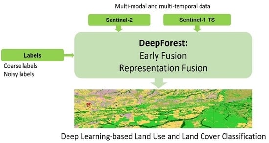
DeepForest: Novel Deep Learning Models for Land Use and Land Cover Classification Using Multi-Temporal and -Modal Sentinel Data of the Amazon Basin

Abstract

Land use and land cover (LULC) mapping is a powerful tool for monitoring large areas. For the Amazon rainforest, automated mapping is of critical importance, as land cover is changing rapidly due to forest degradation and deforestation. Several research groups have addressed this challenge by conducting local surveys and producing maps using freely available remote sensing data. However, automating the process of large-scale land cover mapping remains one of the biggest challenges in the remote sensing community. One issue when using supervised learning is the scarcity of labeled training data. One way to address this problem is to make use of already available maps produced with (semi-) automated classifiers. This is also known as weakly supervised learning. The present study aims to develop novel methods for automated LULC classification in the cloud-prone Amazon basin (Brazil) based on the labels from the MapBiomas project, which include twelve classes. We investigate different fusion techniques for multi-spectral Sentinel-2 data and synthetic aperture radar Sentinel-1 time-series from 2018. The newly designed deep learning architectures—DeepForest-1 and DeepForest-2—utilize spatiotemporal characteristics, as well as multi-scale representations of the data. In several data scenarios, the models are compared to state-of-the-art (SotA) models, such as U-Net and DeepLab. The proposed networks reach an overall accuracy of up to 75.0%, similar to the SotA models. However, the novel approaches outperform the SotA models with respect to underrepresented classes. Forest, savanna and crop were mapped best, with F1 scores up to 85.0% when combining multi-modal data, compared to 81.6% reached by DeepLab. Furthermore, in a qualitative analysis, we highlight that the classifiers sometimes outperform the inaccurate labels.

1. Introduction

Large rainforests significantly influence Earth and atmosphere dynamics, not only by regulating the water cycle but also by balancing the carbon dioxide budget [1]. Rainforests store approximately two billion tons of CO₂ per year and produce about 20% of the Earth’s oxygen [2]. Thus, deforestation is regarded as a critical accelerator of carbon release into the atmosphere. This led to 9% of annual global emissions between 2004 and 2013 [3,4]. Additionally, the biodiversity in the Amazon basin, amounting to a third of the world’s species [5,6], is endangered by ongoing deforestation and land cover change. Several factors, including socioeconomic reasons and political decisions, contribute to the conversion of Amazon forest to non-forest areas. Monitoring changes is critically important to assess damage and provide continuous data for political decision-making and climate and biomass modeling, as well as estimations of age and land cover history. Since 1988, the deforestation-monitoring program PRODES [7] has been conducting annual deforestation mapping for Amazon forest management. This initiative contributed to a record low deforestation rate of 4500 km² per year in 2012 [3,7]. Since then, this number has been constantly rising, with 13,235 km² in 2021 [7].

Over the last few decades, passive and active remote sensing have been investigated for large-scale monitoring. The use of passive remote sensing data for land use and land cover (LULC) classification dates back to 1940, when [8] described the aerial photography mapping of the United States. Landsat was launched in 1972 with multispectral scanners, opening up new possibilities, such as multi-modal data fusion and multi-temporal land cover mapping [9]. Data from the Landsat mission are used, for instance, in the PRODES project [7]. Since 2015, multispectral Sentinel-2 data with higher spatial, spectral and temporal resolutions, compared to Landsat, have been freely available from the Copernicus program. The Copernicus program also freely provides synthetic aperture radar (SAR) data from the Sentinel-1 mission. Therefore, such unprecedented sources of data might prove advantageous and provide promising synergies for land cover mapping, particularly in tropical areas where continuous spectral time-series are rarely available due to cloud cover.

SAR data, as well as multi-spectral data, are used extensively for LULC mapping, forest applications and crop identification. In [10], for example, the authors describe an approach to map forest structural changes using multi-temporal Sentinel-1 images (C-band) with dual polarization over a Scottish forest. In another recent article, [2] described a new, large-scale land-cover mapping methodology in Rondonia. The authors extended the technique already presented in [11] by combining multi-temporal backscatter and interferometric information from repeat-pass short time-series. This resulted in an overall accuracy (OA) of 91.85% using a benchmark land cover map product from 2012 as ground-truth reference. In another study, [12] achieved an OA of 91.5% using random forest (RF) [13] with Sentinel-2 and Sentinel-1 data for 13 different land cover classes in a tropical area. They obtained the best results by combining data from one Sentinel-2 image and eight Sentinel-1 scenes.

From a methodological perspective, machine learning (ML) techniques have been widely used for LULC applications [12,14,15]. Support vector machine (SVM) and RF represent the most popular non-parametric supervised classifiers and outperform previously used classifiers, such as maximum likelihood classification (MLC), k-nearest neighbors (kNN) and classification and regression tree (CART) [9]. RF is popular for its simplicity and its capability to produce robust models and is employed for different applications, such as land cover classification [15]. Many traditional workflows employing ML include extensive feature engineering prior to classification. For instance, the normalized difference vegetation index (NDVI) and other indices are popular feature engineering approaches prior to supervised classification [16,17,18]. Spectral mixture analysis (SMA) can also be employed for feature extraction from multispectral data. For example, [19] used imagery of the Brazilian Amazon captured by the Landsat Thematic Mapper (TM) and Enhanced Thematic Mapper (ETM+) and applied a knowledge-based decision tree to classify forest cover change based on four end members (EMs) extracted from SMA.

In recent years, deep learning (DL) has become very popular for complex classification problems with large datasets. Due to their multilayered structure with nonlinear activation functions, DL models are able to extract hierarchical features from raw data. Each layer learns a more complex and abstract representation from the prior layer [9]. Convolutional neural networks (CNNs) were introduced by [20] and are especially suited for image classification and segmentation problems in computer vision as they can learn spatial features in images. Recently, these methods have become very popular in the remote sensing community [21,22]. In [23] a comprehensive overview is provided with a current review about semantic segmentation using deep learning methods. In [24], seven off-the-shelf deep learning models, such as ResNet50 and InceptionResNetV2, were investigated for a complex land cover classification using RapidEye data with a focus on wetlands in Canada. All deep learning models performed significantly better with respect to OA compared to RF and SVM models trained on the same data. InceptionResNetV2 showed the best performance with an OA of 96.17%.

The inherent challenge of ground-truth data continues to hamper advancements in LULC applications. Recently, [25] presented a weakly supervised approach for investigating state-of-the-art (SotA) methods, such as RF, U-Net and DeepLab, with a fused dataset (SEN12MS) [26]. This dataset combines dual-polarimetric Sentinel-1 and Sentinel-2 imagery. MODIS data with a spatial resolution of 500 m were used as weak reference data (coarse resolution). Ten different land cover classes were identified worldwide, following the simplified International Geosphere–Biosphere Programme (IGBP) classification scheme [27]. The experimental results show that U-Net gives the best results with this particular dataset, with an OA of 48.1%. Such findings pave the way for future research into the capabilities of deep learning approaches.

However, the automatic detection of land use classes after deforestation in the Amazon basin remains challenging. Most of the existing studies in the area are based on mono-temporal satellite data [28] where the data lack the spatiotemporal information that might enable the detection of subtly changing patterns of land cover. This paper aims to investigate the performance of SotA DL algorithms and proposes novel architectures with time-series Sentinel-1 and Sentinel-2 data from the Amazon basin. The proposed novel architectures are tailored to the unique characteristics of the spatiotemporal information of satellite data. We propose various data fusion approaches and investigate the effect of limiting the time-series to only critical periods in terms of vegetation change. We demonstrate the effect of multi-modal data fusion, as well as the potential and drawbacks of weakly supervised learning approaches, in a series of experiments.

2. Materials and Methods

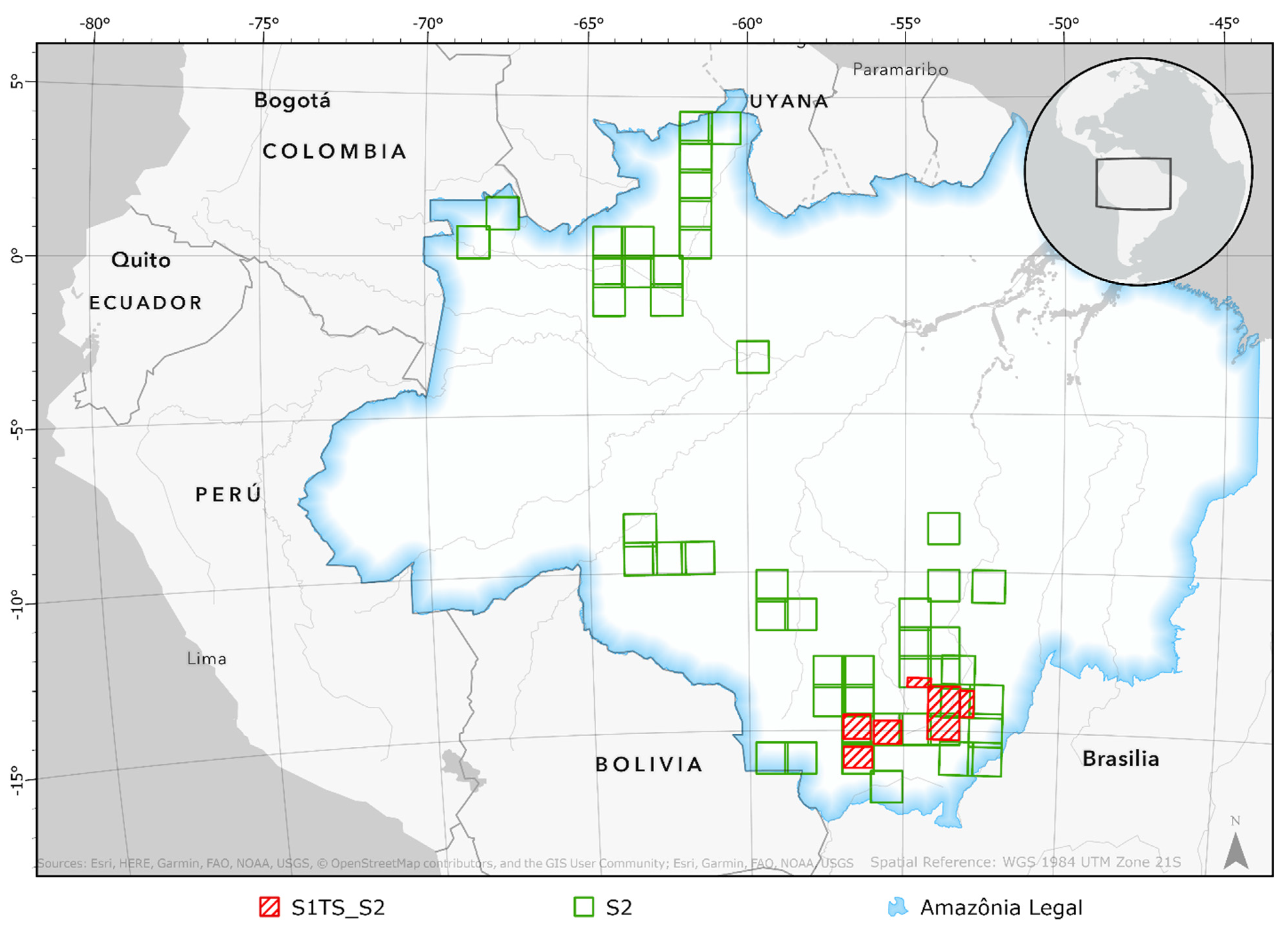
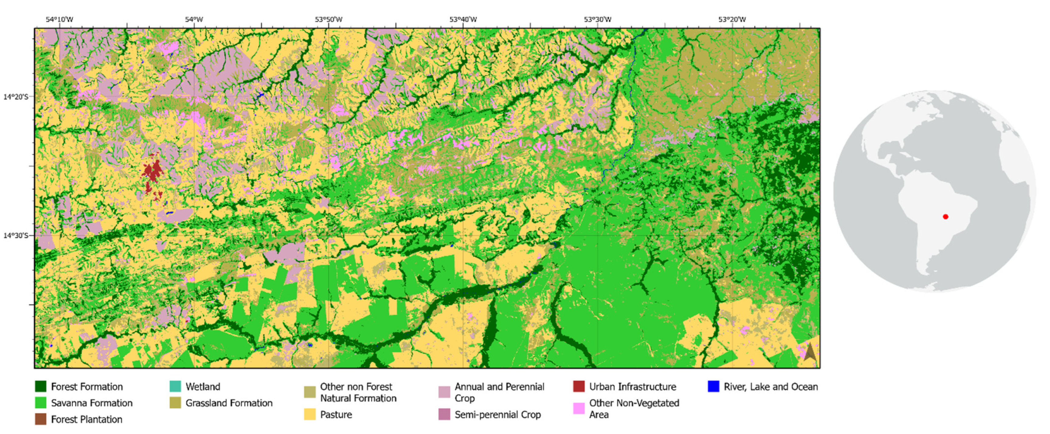
The overall workflow of our study is shown in Figure 1. After extensive pre-processing of Sentinel-1 and Sentinel-2 data (described in Section 3.2), we investigated different SotA architectures and propose new models for our data. The models were implemented in Tensorflow in combination with Keras and additionally integrated into a graphical user-interface in ArcGIS Pro.

2.1. Study Area

The Amazon basin is a world natural treasure representing the largest continuous tropical rainforest in the world, spanning an area of more than 4 million km² [19]. It spreads across nine countries, with 63% of it located in northern Brazil [29]. Amazonia and Mato Grosso are among the states most affected by deforestation. In 2018, they had total forest losses of 1045 km² and 1490 km², respectively [7], and, therefore, significant land cover change. Mato Grosso is situated in the central west of the country and has a well-defined wet season controlled by the South American monsoon system (SAMS), which lasts from September/November to April/May [30]. The annual rainfall in the Amazon can exceed 365 cm/year [31] and occurs mainly during the rainy season. The highest precipitation rates occur in the northwest of the basin and they decrease towards southern regions. As we used multi-spectral satellite data, regions in Mato Grosso were mostly included due to the favorable climate conditions (cf. Figure 2). Mato Grosso is the third largest state in Brazil with three million inhabitants and the main national agricultural producer [32]. The state has very dynamic land cover as it has been suffering from forest degradation and deforestation caused by urbanization and agricultural production [33]. The main crops are soybeans, cotton, corn (maize), sugarcane and sunflower. Therefore, inclusion of time-series data can help differentiate crop classes from other land cover types. Due to the high spatial dynamicity in the area and the confounding vegetation types, visually annotated labels are logistically not feasible in satellite imagery. We adopted the LULC classification scheme used within the MapBiomas project [16]. Overall, the study area comprises 13 different land cover classes, such as forest, pasture, water, urban and crop-related classes. Considering the dominance of forested areas in the area of interest, there are strong imbalances in the representation of the LULC classes (e.g., crops, urban), which was a major challenge in this study. However, such a diverse ecosystem is a good real-world opportunity to investigate the performance of DL models with satellite data.

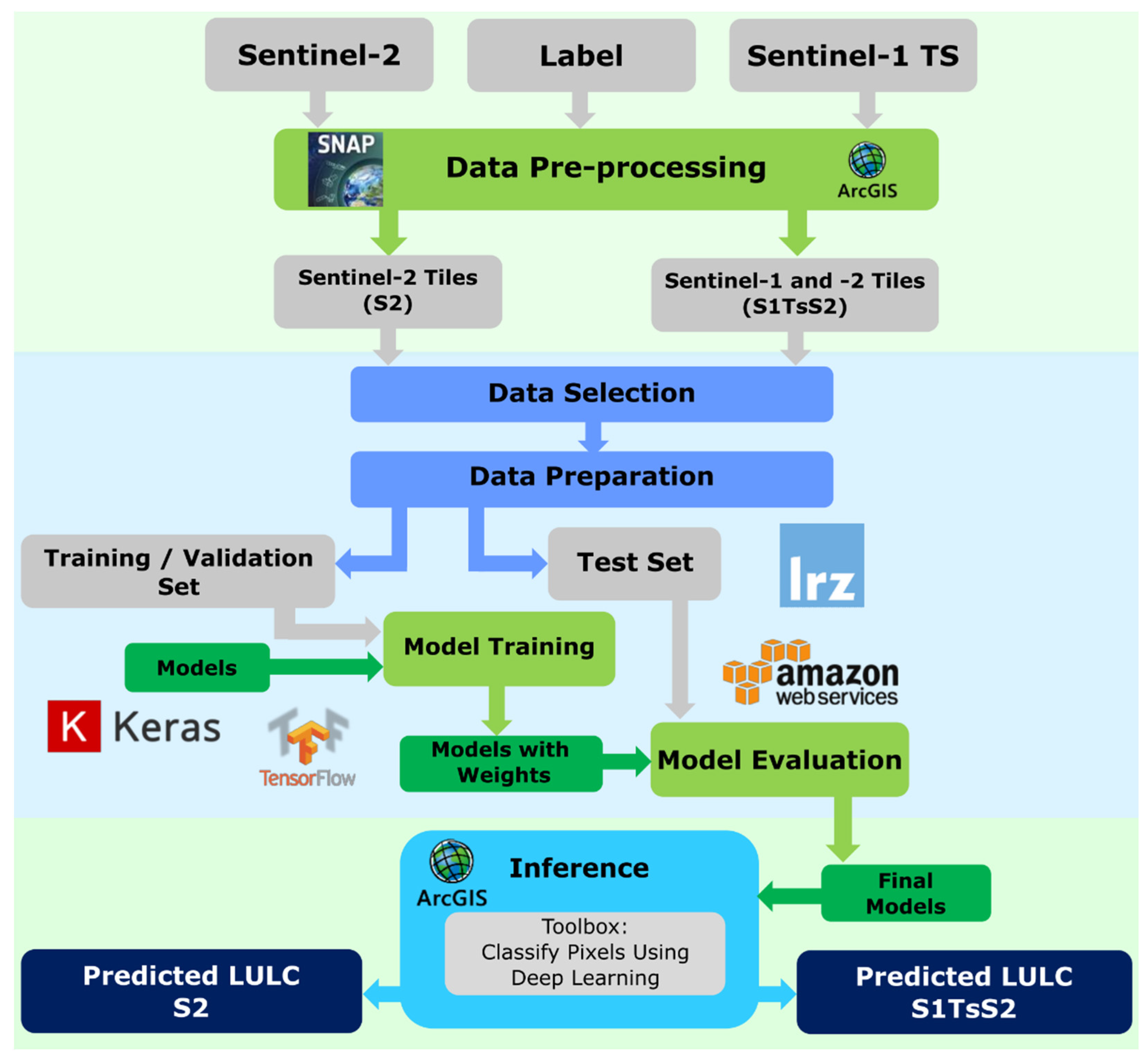
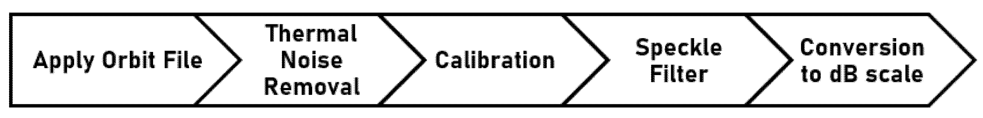
2.2. Data and Pre-Processing

We used 48 Sentinel-2 scenes and 24 Sentinel-1 scenes (representing two time-series) across Amazonia and Mato Grosso, with their locations shown in Figure 2. Only Sentinel-2 images with a total cloud cover of less than 10% were acquired and most of the scenes were downloaded as Bottom-Of-Atmosphere (BOA) Level-2A products. The remaining scenes were only available as Top-Of-Atmosphere (TOA) Level-1C products and atmospherically corrected to BOA reflectance using the Sen2Cor toolbox in SNAP. To obtain the best configuration for generating the L2A product, we used auxiliary data from the surfaces of the Climate Change Initiative (CCI) Land Cover data from 2015 provided by the European Space Agency (ESA).

Sentinel-2 consists of 13 spectral bands ranging from the visible (443 nm) to infrared (2190 nm), with spatial resolutions of 10, 20 or 60 m. The three 60 m bands for atmospheric applications were omitted in this study. The six 20 m bands were then resampled to 10 m using the nearest neighbor method.

Sentinel-2 data are well-suited for LULC classification due to the improved spectral resolution compared to, for example, the Landsat missions. However, for tropical regions, it is hard to obtain cloud-free data and, therefore, multi-temporal classification for large areas using only this data is not feasible. To overcome this limitation, we included Sentinel-1 SAR time-series from 2018. The time-series contain one scene per month with two polarizations, resulting in 24 scenes. All scenes were acquired as Level-1 GRD products, captured as dual-polarized interferometric wide swath (IW) images (VH + VV). Further pre-processing was conducted using ESA’s SNAP application. The processing workflow comprised orbit correction, thermal noise removal, calibration, filtering of the speckle effect using a Lee filter and conversion of the values to a dB scale (cf. Figure 3).

After pre-processing, the Sentinel-1 time-series and the Sentinel-2 spectral data were stacked into a single image cube with 34 bands for the selected areas of interest (marked red in Figure 2). Three datasets were exported as labeled image tiles from ArcGIS Pro and were each split into a training and a test dataset: one dataset contained all 34 bands (S1TsS2_12). The second (S1TsS2_7) contained the 10 multispectral bands but only 14 SAR bands corresponding to a time-series of 7 months (June–December), as this time frame showed a slightly better class distinction from a separate analysis on the backscatter signal. The third dataset covered a larger area but only with the Sentinel-2 bands (S2). The datasets are summarized in

Table 1. The different subsets built from the S2 and S1TsS2 datasets.

Dataset	Number of Tiles		Number of Bands	Tile Size [px]
	Training	Test
S2	35,000	8750	10	256 × 256
S1TsS2_12	18,074	4517	34	256 × 256
S1TsS2_7	18,074	4517	24	256 × 256

. Due to computational limitations, the Sentinel-1 time-series could not be processed at the same spatial extent as Sentinel-2 data (see Figure 2 for details).

As labels, we used data from the MapBiomas Project [16]. The project provides six sets of annual maps generated with different techniques, ranging from empirical decision trees to RF classifiers, all based on Landsat imagery. We used their classification map data (collection 4) from 2018, as this was the most current iteration at the start of our project. The global accuracies for the land cover classes in the MapBiomas project range from 70% to 94%, varying across regions [34]. Thus, the labels used were noisy and cannot be considered real ground-truth. In addition, they were derived from a coarser spatial resolution than the Sentinel-2 and Sentinel-1 sensors and did not, therefore, exactly line up with respect to our data. These challenges match with the latter two of the three types of weak supervision described by [35]: incomplete (missing labels), inexact (coarser resolution), and inaccurate (noisy labels). They suggest still making use of inaccurate and inexact labels to produce good models and investigate techniques to overcome these problems.

Another challenge of our data was class imbalance: in the large study area (S2), there were 3 dominant classes among the 13 total classes: forest formation (FF), pasture and savanna, which had pixel distributions of 42.7%, 20.6% and 15.8%, respectively. Four other classes had pixel percentages ranging between 4% and 9%. All remaining classes were underrepresented and added up to approximately 1%. In the smaller S1TsS2 dataset, there were five dominant classes: savanna, pasture, FF, annual and perennial crop (A&C crop) and grassland, with pixel coverage percentages of 30%, 23%, 16%, 11% and 10%, respectively. The remaining classes’ coverage percentages were up to 5%.

2.3. Deep-Learning Approaches and Experiments

As described in the previous section, there were challenges with respect to our data and labels. Therefore, we conducted several experiments with the goal of investigating potential SotA architectures used in computer vision, as well as new approaches applied to multi-temporal data. The experiments tackling the different challenges can be summarized as follows:

• Investigation of the performance of SotA architectures with Sentinel-2 and SAR Sentinel-1 data regarding LULC classification. We trained and tested U-Net and DeepLab on both the multispectral data and the fused datasets;
• Furthermore, we propose new approaches including spatial-temporal dependencies and different fusion strategies to take the multi-temporal nature of the data into consideration;
• Finally, we compared the results obtained from different data combinations used in all experiments.

All models were implemented in Tensorflow in combination with Keras. All training was performed on two virtual machines at the Leibniz-Rechenzentrum (LRZ) and at Amazon Elastic Cloud (EC2). The machine configurations are summarized in

Table 2. Technical details about the developing and testing environments.

	LRZ	EC2
GPU (Memory)	NVIDIA V100 (16 GB)	NVIDIA T4 (16 GB)
RAM (GB)	500	200
Operating System	Linux	Windows
DL Framework	Tensorflow 1.15.2 + Keras

. The trained models were then integrated into a GUI in ArcGIS Pro to provide an easy interface for inference with new datasets.

The data were randomly split into training, validation (20% of the training set) and test sets. Additionally, to prevent overfitting, we used data augmentation (horizontal flipping and rotation of 2000 tiles) and early stopping. Initially, the model training process was fixed to 10 epochs. With the control of the validation accuracy, early stopping was forced if the validation loss did not decrease anymore.

2.3.1. State-of-the-Art Architectures

We used two SotA methods for semantic segmentation to compare to our new proposed models: U-Net [36] and DeepLab [37]. U-Net was developed in 2015 for biomedical image segmentation. The architecture consists of symmetric down- and up-sampling levels of feature maps with skip connections. The idea of down-sampling (encoder) and up-sampling (decoder) paths was initially introduced with fully convolutional networks (FCNs) [38] to circumvent the loss of information about the object location after the convolution. For model development, we used a modified version of U-Net, following [39], with four down- and up-sampling blocks.

DeepLab [37] is one of the most popular models in computer vision and uses a dilated convolutional operation (coined the “atrous” operator). This technique has been used in signal processing to efficiently compute the undecimated wavelet transform. Atrous convolution makes it possible to enlarge the field of view of filters without increasing the number of parameters to be learned or the computation time. Thus, the idea is to use larger kernel sizes for convolution by introducing zero values, called holes, or a dilation rate between the filter values. This drastically reduces the number of learnable weights. The Atrous Spatial Pyramid Pooling (ASPP) module is the second useful addition in this model. This method is used to robustly produce image representations of objects at multiple scales by concatenating the feature maps extracted from different dilation rates to obtain the final feature map [37]. The implementation of this model is based on ResNet50 [40] as the backbone architecture.

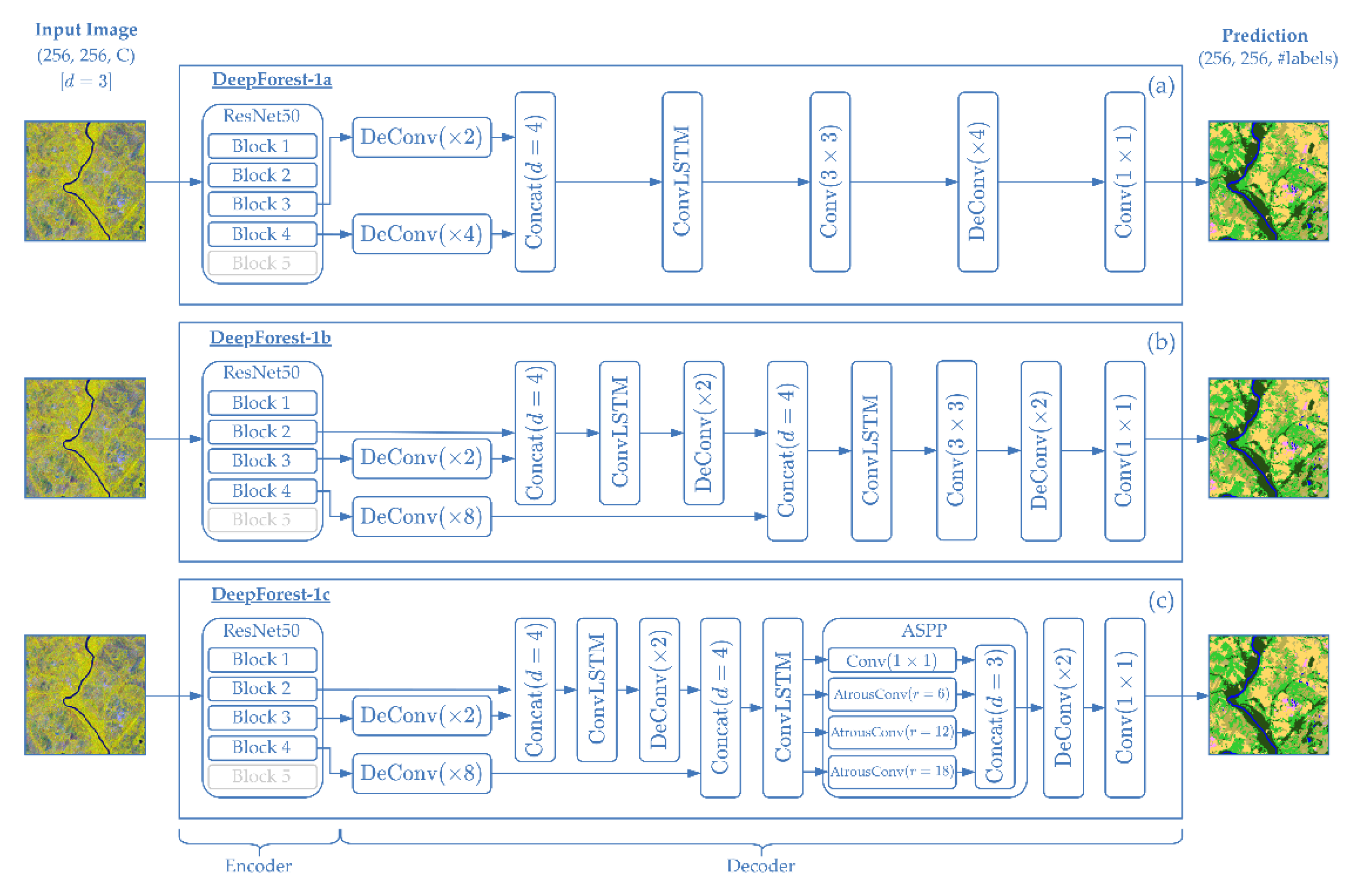
2.3.2. Early Fusion Approach: DeepForest-1

We propose new architectures for data fusion that take the multi-temporal and multi-modal nature of the data into consideration. The architectures are inspired by the FCN architecture [38], as well as the ConvLSTM unit [41].

We tested three model variations for this approach, which are described in the following and shown in Figure 4. As the FCN architecture merges the skip-connection layers by summation, the proposed DeepForest-1 architecture additionally introduces layer merging through the use of ConvLSTM [41] blocks. This can improve the way the network learns features and propagates them throughout the architecture. Fusing skip connections with a linear function (sum) might not consider the correlation between them. Instead, DeepForest-1 takes advantage of the properties of LSTM, through ConvLSTM, to select and keep the relevant features from the introduced maps in memory. Thus, the model has a robust representational power to learn nonlinear features and avoid redundancy. As with most of the semantic segmentation models, DeepForest-1 also employs an encoder/decoder structure.

Encoder path: As an encoder, ResNet50 [40] is used as the backbone and comprises five blocks of convolutional units. However, in this study, only the first four of the five blocks are used. Each consists of convolutional layers with batch normalization and ReLU activation units. The batch normalization layers compensate for the instability of the neural network, which is caused by the distribution variation of the activation values after each layer. This layer therefore regularizes the inputs to each layer by normalizing each batch [42].

ConvLSTM block: The ConvLSTM unit was introduced by [41] as a generalization of LSTM [43]. It considers the spatiotemporal correlations of image data rather than just the temporal correlation. The block produces an output feature map for each of the pixel positions by taking the inputs and the previous states of the surrounding pixels into account. The key operations [41] of this block are shown in the following equations, where $W$ are the learned weights of the block and $\left(\otimes \right)$ represents the Hadamard product:

$$\hspace{1em}\hspace{1em}\hspace{1em}{f}_t=\sigma \left(W_{xf}\ast X_t+W_{hf}\ast H_{t-1}+W_{cf}\otimes C_{t-1}+b_f\right) \mathrm{Forget} \mathrm{gate} \mathrm{at} \mathrm{time} t$$

(1)

$$\hspace{1em}\hspace{1em}\hspace{1em}{i}_t=\sigma \left(W_{xi}\ast X_t+W_{hi}\ast H_{t-1}+W_{ci}\otimes C_{t-1}+b_i\right) \mathrm{Input} \mathrm{gate} \mathrm{at} \mathrm{time} t$$

(2)

$$\hspace{1em}\hspace{1em}\hspace{1em}{o}_t=\sigma \left(W_{xo}\ast X_t+W_{ho}\ast H_{t-1}+W_{co}\otimes C_{t-1}+b_o\right) \mathrm{Output} \mathrm{gate} \mathrm{at} \mathrm{time} t$$

(3)

$$\hspace{1em} \hspace{1em}\hspace{1em}\hspace{1em}\widetilde{C_t}=\tan \mathrm{h}\left(W_{xc}\ast X_t+W_{hc}\ast H_{t-1}+b_c\right)\hspace{1em}\hspace{1em}\hspace{1em}\hspace{1em}\mathrm{Carry} \mathrm{candidate} \mathrm{at} \mathrm{time} t$$

(4)

$$\hspace{1em} C_t=i_t\otimes \widetilde{C_t}+C_{t-1}\otimes f_t\hspace{1em}\hspace{1em}\hspace{1em}\hspace{1em}\hspace{1em}\hspace{1em}\hspace{1em}\hspace{1em}\hspace{1em}\hspace{1em}\mathrm{New} \mathrm{carry} \mathrm{at} \mathrm{time} t$$

(5)

$$\hspace{1em}{H}_t=o_t\otimes \tan \mathrm{h}\left(C_t\right)\hspace{1em}\hspace{1em}\hspace{1em}\hspace{1em}\hspace{1em}\hspace{1em}\hspace{1em}\hspace{1em}\hspace{1em}\hspace{1em}\hspace{1em} \mathrm{Output} \mathrm{at} \mathrm{time} t$$

(6)

The formulation is similar to the LSTM unit, but it includes spatial correlation using the convolution operator $\left(\ast \right)$ rather than simple multiplication. Similarly, each unit of ConvLSTM comprises three gates (forget $f_t$, output $o_t$ and input $i_t$), as well as two states (memory cell state $C_t$ and hidden state $H_t$), characteristic elements for an LSTM unit. These elements allow not only the propagation of regulated information (to hold or forget) but also the prevision of the vanishing gradients. In the context of recurrent neural networks (RNNs), the feature maps extracted from different levels are treated as images with different timestamps in the new designed architecture (RNNs). The ConvLSTM therefore produces a new representation segment from the two introduced feature maps.

Decoder path: The decoder path consists of a succession of up-convolutional layers to recover the initial spatial resolution. The skip connections from the encoder path are merged with the up-convoluted feature maps through concatenation and ConvLSTM blocks. The merging of features from different resolutions aids in the combination of context information and spatial information, as well as the reconstruction of the spatial resolution of the initially introduced image [38]. The rest of the model consists of a final convolution layer using Softmax as the activation function.

Model Variations: We propose three modifications to the model, the first with one ConvLSTM unit (DeepForest-1a), the second with two units to include a lower layer below the encoder (DeepForest-1b) and a final version with atrous convolution and an additional ASPP block (DeepForest-1c). The architectures of these three models are shown in Figure 4. The first model variation (DeepForest-1a) introduces a ConvLSTM block that merges the feature maps from block 3 (with a size of 32 × 32) and block 4 (with dimensions of 16 × 16) of the encoder backbone (ResNet50). The dimensions of each feature map have to be up-sampled first to 64 × 64 in order to then enter the ConvLSTM unit (see Figure 4a). The second variation (DeepForest-1b) concatenates the outputs from block 2 (64 × 64) and block 3 (32 × 32) of the encoder and then merges the resulting output of the ConvLSTM unit (64 × 64) with the output from block 4 (16 × 16) (cf. Figure 4b). The third version (DeepForest-1c) is analogous to the second model variation but introduces an ASPP block that was initially introduced in the DeepLab [37] architecture. This block is added at the end of the architecture to test the effect of the multiple scale map generation on our data (see Figure 4c).

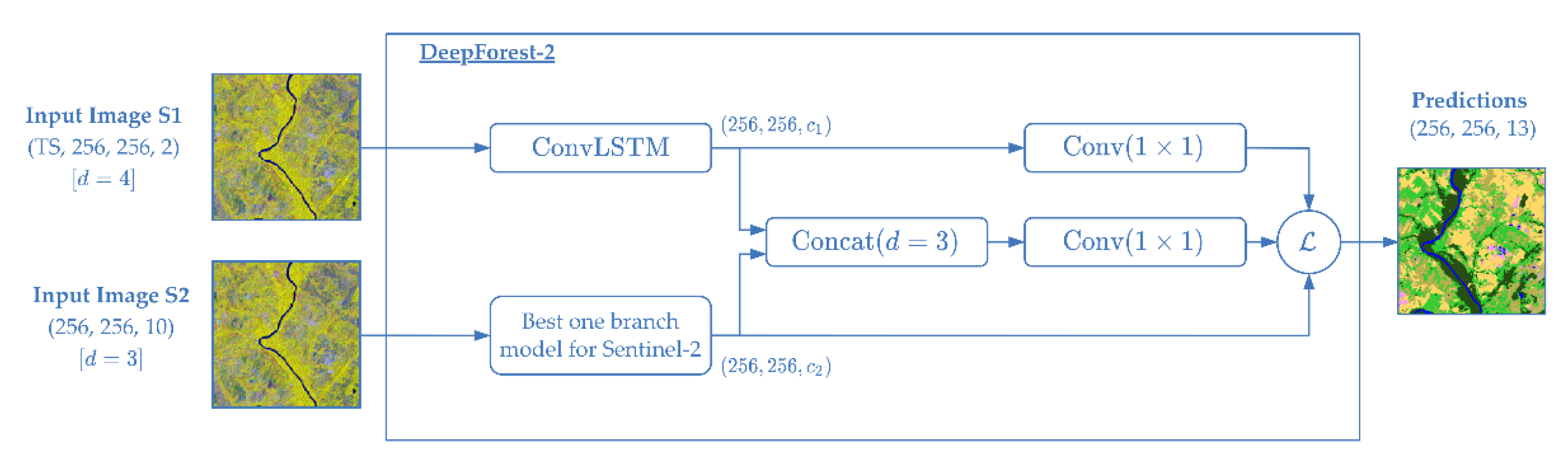
2.3.3. Representation Fusion: DeepForest-2

Designing two-branch models was another approach taken to investigate the effect of fusion of Sentinel-1 and Sentinel-2 data. Each of the streams has its own architecture (Figure 5) that learns sensor-specific representations. The stream responsible for multi-spectral data (S2) consists of either U-Net (DeepForest-2a) or DeepForest-1b (DeepForest-2b), while the second stream contains one ConvLSTM block for time-series Sentinel-1 (TS S1). This allows the model to learn features from both modalities separately. The final produced feature maps from both branches are concatenated to form the new global model (DeepForest-2). The training process of the global model and the separate branches are intertwined. The contribution of each stream is weighted differently in the final loss function$L$. In our experiments, we assigned a higher weight to the Sentinel-2 branch with 70%, given the high correlation of spectral information with land cover classes, while 30% was assigned for Sentinel-1.

2.3.4. Loss Function

The most commonly used loss function for multiclass segmentation is the categorical cross-entropy (CCE).

$$\mathrm{CCE}\left(\widehat{y},y\right)=-\frac{1}{N} {\displaystyle \sum }_{i=1}^N{\displaystyle \sum }_{j=1}^C{y}_{i,j}·\log \left(p\left({\widehat{y}}_{i,j}\right)\right)$$

(7)

$N$ represents the number of samples and $C$ is the number of classes. The value $\widehat{y}$ represents the predicted class, with $y$ being the expected class; i.e., the training label. The predicted labels are normalized with the Softmax function $p\left(x\right)=e^x/{{\displaystyle \sum }}_{c=1}^C{e}^{x_c}$. To compensate for the problem of class imbalance, one solution is to use a weighted loss function. The weights are calculated per class from the training set labels and represent the complementary respective percentage of the number of pixels for every class (NPC%). Well-represented classes have lower weights and underrepresented classes have higher weights. In all the experiment cases, we consider the weighted version of the loss functions.

$$\mathrm{Class} \mathrm{weights} =100 - \mathrm{NPC}\%$$

(8)

2.4. Evaluation Metrics

The OA and the class-wise accuracies are commonly used metrics to evaluate the performance of deep neural networks. The OA is derived from the values of the confusion matrix (TP: true positive, TN: true negative, FP: false positive and FN: false negative):

$$\mathrm{OA}=\frac{\mathrm{TP}+\mathrm{TN}}{\mathrm{TP}+\mathrm{TN}+\mathrm{FP}+\mathrm{FN}}$$

(9)

However, as the OA reports the number of correctly assigned pixels over the total number, it does not represent the model’s performance well in scenarios with class imbalance and favors the dominant classes. Therefore, we also report the intersection over union (IoU) (10) and the F1 score (11). IoU represents the proportion of correctly classified pixels to the total number of pixels between the reference and the resulting classification. F1 represents the harmonic mean of the precision and the recall metric and, thus, can be interpreted as the trade-off measure between both metrics.

$$\mathrm{IoU}=\frac{\mathrm{TP}}{\mathrm{TP}+\mathrm{FP}+\mathrm{FN}}$$

(10)

$$\mathrm{F}1=2\cdot \frac{\mathrm{Precision}\cdot \mathrm{Recall}}{\mathrm{Precision}+\mathrm{Recall}}=\frac{\mathrm{TP}}{\mathrm{TP}+\frac{1}{2\cdot \left(\mathrm{FP}+\mathrm{FN}\right)}}$$

(11)

3. Results

In the following sections, we present the quantitative results of the experiments described in the previous section. In addition, we also describe the qualitative analysis, as quantitative metrics are not completely reliable due to the problem of inaccurate labels in the maps produced by the models.

3.1. Quantitative Results on Multispectral Data

U-Net reached the highest OA among all the models (77.9%) classifying Sentinel-2 data (

Table 3. Test accuracies of the classifications based on multispectral data (S2 dataset) for SotA and DeepForest-1 models. Abbreviations: DF = DeepForest, DLab = DeepLab, UN = U-Net, FF = forest formation, FP = forest plantation, A&P Crop = annual and perennial crop, oN-FNF = other non-forest natural formation, oN-VNA = other non-vegetated area, SP Crop = semi-perennial crop.

	F1 [%]				IoU [%]
	UN	DLab	DF 1a	DF 1b	UN	DLab	DF 1a	DF 1b
FF	92.0	90.1	87.7	91.2	85.1	82.0	78.2	83.8
Savanna	65.8	60.5	41.2	39.7	49.0	43.4	26.0	24.7
FP	0.0	2.8	0.0	0.0	0.0	1.4	0.0	0.0
Wetland	0.0	0.0	0.0	0.0	0.0	0.0	0.0	0.0
Grassland	48.8	38.6	25.5	21.1	32.3	23.9	14.6	11.8
oN-FNF	50.4	45.0	33.6	39.5	33.7	29.0	20.1	24.6
Pasture	72.8	64.6	73.2	61.5	57.2	47.7	57.7	44.4
A&P Crop	76.2	54.8	73.5	68.1	61.5	37.7	58.1	51.6
SP Crop	0.0	0.0	0.0	0.0	0.0	0.0	0.0	0.0
Urban	69.4	61.5	0.0	0.0	53.1	44.4	0.0	0.0
oN-VNA	0.3	8.8	2.6	0.0	0.14	4.6	1.3	0.0
Water	86.0	85.7	76.7	78.8	75.4	75.0	62.2	65.0
Macro Average	46.8	42.7	34.5	33.3	37.3	32.4	26.5	27.8
Weighted Average	77.9	71.9	69.9	68.4	66.0	59.1	57.5	56.5
	U-Net			DeepLab	DeepForest-1a		DeepForest-1b
Overall Accuracy [%]	77.9			72.7	72.7		71.4

). However, the model failed to capture all classes: three classes, forest plantation, wetland and semi-perennial crop, were completely omitted by the model and attributed to other classes, as shown in the confusion matrix in Figure 6a. Considering the class accuracies, we observe that U-Net performed well with multispectral data for forest, water and annual crops. However, other classes, such as non-vegetated areas, were not very well captured (cf. Table 3). DeepLab was the second best model and reached an OA of 72.7%, which was 5.2 pp lower than U-Net. Similar to U-Net, this model also exhibited low performance in capturing semi-perennial crop and wetland areas. However, it was able to correctly classify some forest plantation and non-vegetated pixels in the test set. Overall the two SotA models had comparable class accuracies.

With these data settings, SotA models seemed to perform slightly better than DeepForest variations. The newly designed deep learning model, DeepForest-1a, reached the same OA as DeepLab (72.7%) but with different class accuracies. Similarly to U-Net, both DeepForest models failed to detect forest plantation, wetland and semi-perennial crop classes. Additionally, none of the urban infrastructure class samples in the test set were identified correctly (cf. Table 3). However, they still had plausible accuracies for the dominant classes in the selected area. For instance, DeepForest-1a had the highest detection rate for the pasture class, reaching an F1 score of 73.2%, and DeepForest-1a reached the second highest score for forest formation classification (F1 of 91.2%; cf. Table 3)

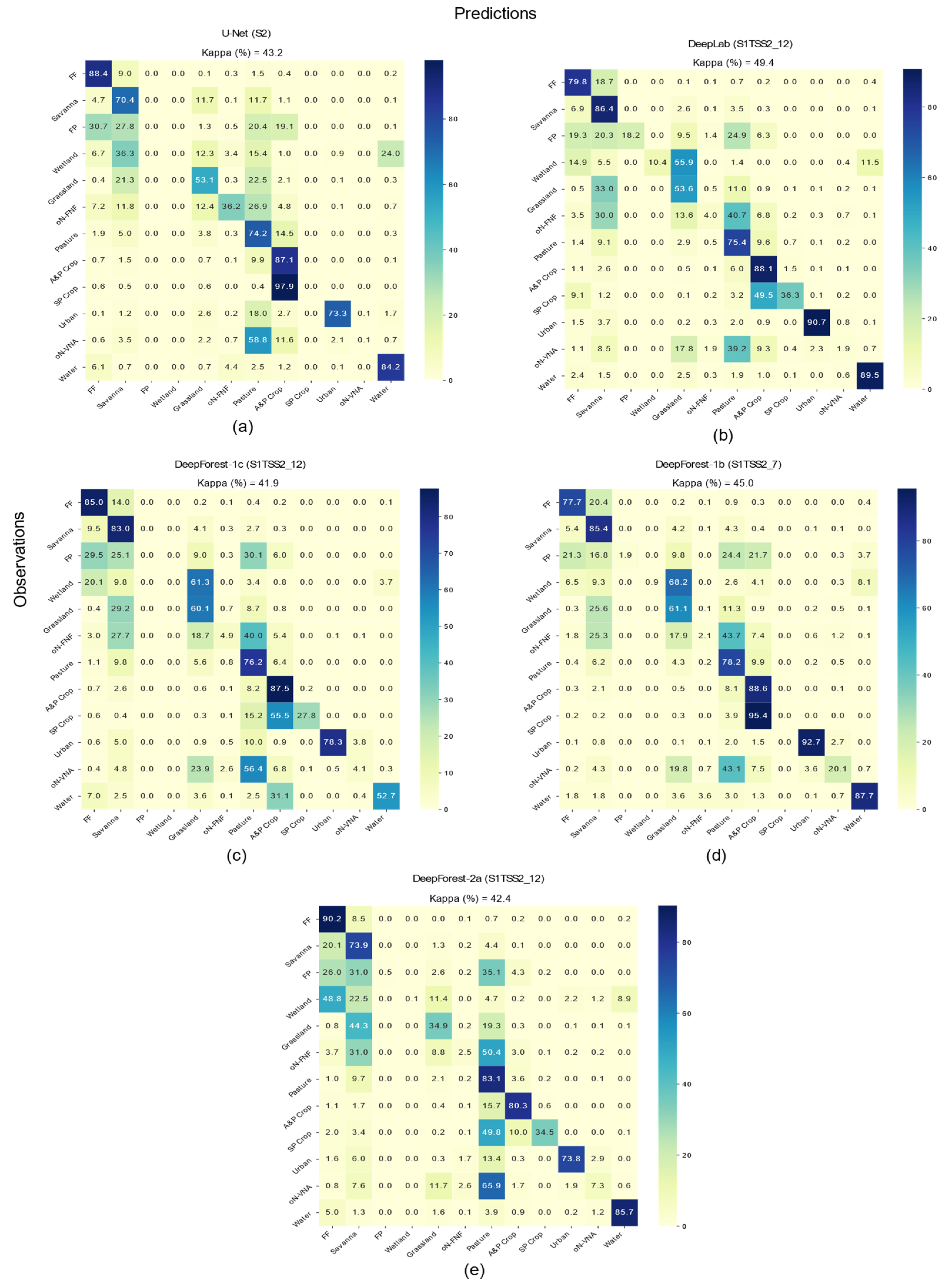
3.2. Quantitative Results on Multi-Modal-Data

The best overall accuracy for purely multi-spectral data slightly outperformed models trained on multi-modal data (note that the datasets did not cover the same area extents; cf. Figure 2). However, U-Net’s performance dropped significantly when introducing the multi-modal dataset that included the Sentinel-1 time series (Table 3 and

Table 4. Test accuracies of the classifications based on multi-modal data (S1TsS2_12 dataset) for SotA and DeepForest models. Abbreviations: DF = DeepForest, DLab = DeepLab, FF = forest formation, FP = forest plantation, A&P Crop = annual and perennial crop, oN-FNF = other non-forest natural formation, oN-VNA = other non-vegetated area, SP Crop = semi-perennial crop.

	F1 [%]							IoU [%]
	UN	DLab	DF 1a	DF 1b	DF 1c	DF 2a	DF 2b	UN	DLab	DF 1a	DF 1b	DF 1c	DF 2a	DF 2b
FF	32.6	80.9	81.5	81.1	82.1	77.5	71.8	19.5	67.9	68.8	68.2	69.7	63.2	56.0
Savanna	60.0	74.4	77.1	74.3	77.8	71.6	73.2	42.8	64.6	62.7	59.1	63.7	55.8	57.7
FP	0.0	30.3	0.0	0.0	0.0	0.9	0.0	0.0	17.9	0.0	0.0	0.0	0.5	0.0
Wetland	0.0	18.1	0.6	0.0	1.8	0.1	5.0	0.0	9.9	0.3	0.0	0.9	0.1	2.6
Grassland	52.2	59.8	58.7	53.0	60.1	46.4	47.2	35.4	42.7	41.5	36.1	43.0	30.2	30.9
oN-FNF	2.6	7.4	3.3	5.6	8.8	4.7	2.2	1.3	3.8	1.7	2.9	4.6	2.4	1.2
Pasture	67.6	75.5	76.4	74.8	76.2	75.3	71.5	51.0	60.7	61.8	59.8	61.5	60.4	55.6
A&P Crop	61.9	81.6	83.6	85.0	83.2	84.1	82.9	44.8	69.0	71.8	73.9	71.3	72.6	70.8
SP Crop	0.0	13.8	0.0	0.4	32.2	26.2	12.0	0.0	7.4	0.0	0.2	19.2	15.1	6.4
Urban	43.0	85.5	88.0	86.5	85.2	77.7	72.7	27.4	74.6	78.6	76.2	74.2	63.5	57.1
oN-VNA	15.0	28.4	21.9	25.8	7.7	12.7	8.0	8.1	16.6	12.3	14.8	4.0	6.8	4.2
Water	84.9	88.8	89.0	88.2	67.6	89.5	88.8	73.8	79.9	80.2	78.9	51.1	81.0	79.8
Macro Average	35.0	54.1	48.3	47.9	48.6	47.2	44.6	25.3	42.9	40.0	39.2	38.6	37.6	35.2
Weighted Average	52.2	69.4	71.0	69.4	71.5	67.1	65.5	37.1	60.6	57.8	55.8	58.3	53.2	51.3
	UN	DLab	DF-1a		DF-1b		DF-1c		DF-2a		DF-2b
Overall Accuracy [%]	56.7	74.4	74.3		72.9		74.4		70.9		69.0

). Overall, the class accuracies for models calibrated with multi-modal data were improved compared to when only using Sentinel-2 data (Table 3 and Table 4). For instance, the mappings of savanna, grassland and annual and perennial crop classes (dominant classes) had the same accuracy patterns as with the mono-modal experiments, even with smaller area extent, but were clearly improved for all models. In particular, the crop sub-class (SP Crop) was mostly better mapped with DeepForest models. Apart from the vegetated areas, the urban, non-vegetated and water classes also improved with more information in the input data. Surprisingly, the accuracies for the forest formation class slightly dropped with all models when introducing SAR data.

The early data fusion approaches (DeepForest-1) seemed to have higher model accuracies than those with the representation fusion (DeepForest-2). DeepForest-1a and DeepForest-1b were able to learn and map, albeit with a low accuracy, some of the complex and underrepresented classes that could not be predicted using only S2 data (e.g., forest plantation and wetland). The best-performing model with early data fusion (DeepLab) reached an average F1 score of 53.7% compared to only 42.7% with multispectral data. The model learned to detect almost all of the existing classes, as shown by the diagonal values of the confusion matrix in Figure 6b.

The atrous convolutions and ASPP block of DeepForest-1c did not improve results significantly, as the model achieved similar scores as DeepLab and DeepForest-1a. The extension of the receptive field through the ASPP block only increased the accuracies of crop and vegetated classes.

3.3. Quantitative Results on Reduced Multi-Modal Data

The results suggest that U-Net is not suitable for classification using multi-modal and multi-temporal data (Table 4). Thus, we only tested DeepLab and DeepForest on the reduced time-series data using just a seven-month time frame, from June to December, instead of all 12 months (

Table 5. Test metrics comparison of DeepForest-1 and DeepLab with different time-series lengths for Sentinel-1 data (S1TsS2_7 vs. S1TsS2_12). Abbreviations: DF = DeepForest, FF = forest formation, FP = forest plantation, A&P Crop = annual and perennial crop, oN-FNF = other non-forest natural formation, oN-VNA = other non-vegetated area, SP Crop = semi-perennial crop.

	F1 [%]								IoU [%]
	DeepLab		DF-1b		DF-1c		DF-2b		DeepLab		DF-1b		DF-1c		DF-2b
	7 Ms	12 Ms	7 Ms	12 Ms	7 Ms	12 Ms	7 Ms	12 Ms	7 Ms	12 Ms	7 Ms	12 Ms	7 Ms	12 Ms	7 Ms	12 Ms
FF	71.2	80.9	81.9	81.1	44.2	82.1	55.2	71.8	55.3	67.9	69.3	68.2	28.4	69.7	38.1	56.0
Savanna	75.8	74.4	79.6	74.3	72.2	77.8	73.4	73.2	61.0	64.6	66.1	59.1	56.5	63.7	58.0	57.7
FP	0.0	30.3	3.7	0.0	0.0	0.0	0.0	0.0	0.0	17.9	1.9	0.0	0.0	0.0	0.0	0.0
Wetland	27.0	18.1	1.7	0.0	0.0	1.8	0.0	5.0	15.6	9.9	0.9	0.0	0.0	0.9	0.0	2.6
Grassland	58.0	59.8	61.9	53.0	60.3	60.1	56.5	47.2	40.8	42.7	44.8	36.1	43.2	43.0	39.4	30.9
oN-FNF	2.0	7.4	4.0	5.6	3.2	8.8	1.3	2.2	1.0	3.8	2.0	2.9	1.6	4.6	0.6	1.2
Pasture	71.9	75.5	76.0	74.8	76.1	76.2	73.8	71.5	56.0	60.7	61.3	59.8	61.4	61.5	58.5	55.6
A&P Crop	74.1	81.6	81.3	85.0	83.1	83.2	79.5	82.9	58.8	69.0	68.6	73.9	71.0	71.3	66.4	70.8
SP Crop	0.1	13.8	0.0	0.4	0.1	32.2	0.0	12.0	0.0	7.4	0.0	0.2	0.0	19.2	0.0	6.4
Urban	79.0	85.5	80.3	86.5	84.6	85.2	71.2	72.7	65.3	74.4	67.1	76.2	73.3	74.2	55.3	57.1
oN-VNA	18.0	28.4	26.8	25.8	23.9	7.7	26.1	8.0	9.9	16.0	15.5	14.8	13.6	4.0	15.0	4.2
Water	86.0	88.8	67.6	88.2	88.9	67.6	89.3	88.8	76.0	79.9	80.1	78.9	79.5	51.1	80.6	79.8
Macro Average	46.9	53.7	47.1	47.9	44.7	48.5	43.9	44.6	36.6	42.9	39.8	39.2	35.7	38.6	34.3	35.2
Weighted Average	67.5	71.0	72.6	70.4	64.3	72.2	65.0	66.5	52.9	58.8	59.6	56.7	50.0	58.9	50.4	52.1
	DeepLab				DeepForest-1b				DeepForest-1c				DeepForest-2b
	7 Months		12 Months		7 Months		12 Months		7 Months		12 Months		7 Months		12 Months
Overall Accuracy [%]	69.9		74.4		75.0		72.9		67.8		74.4		68.1		69.0

). DeepForest-1b achieved the best results with an OA of 75% for the reduced time-series, while the other models exhibited decreases in their OAs (cf. Table 5). Interestingly, the detection of classes such as forest formation, savanna and wetland slightly improved using the shorter time-series. However, crop classes seem to benefit the most from longer time-series.

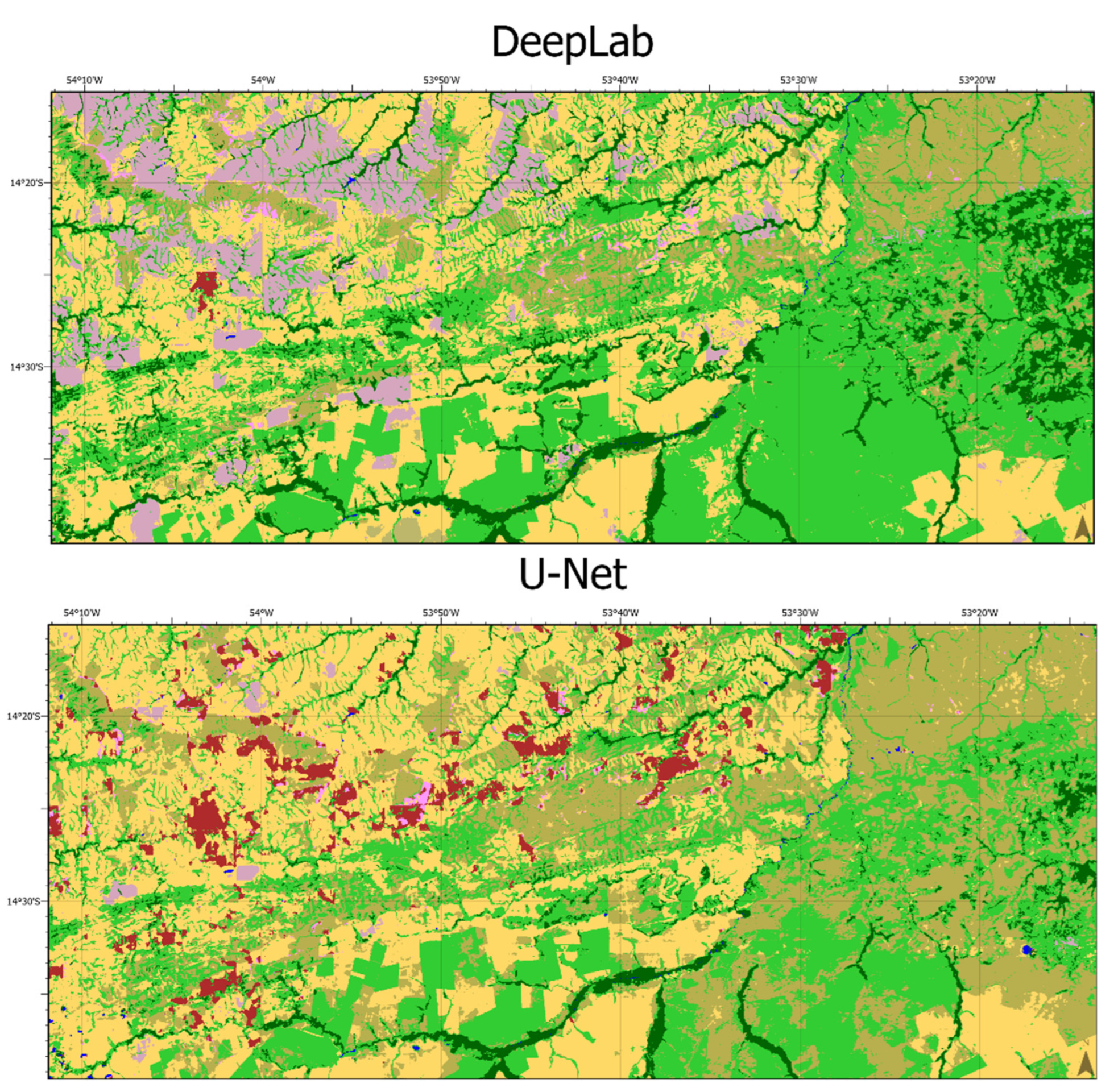
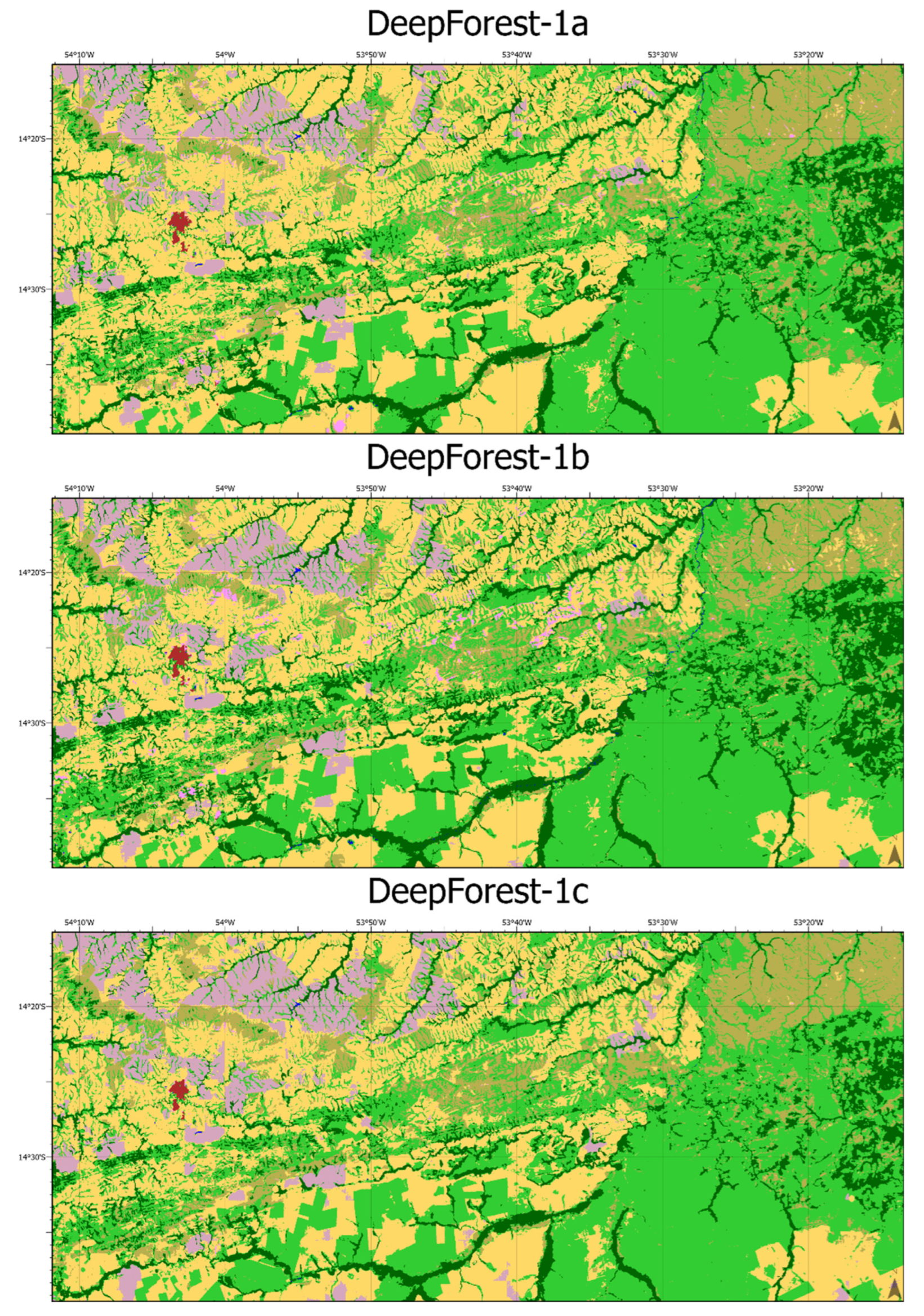
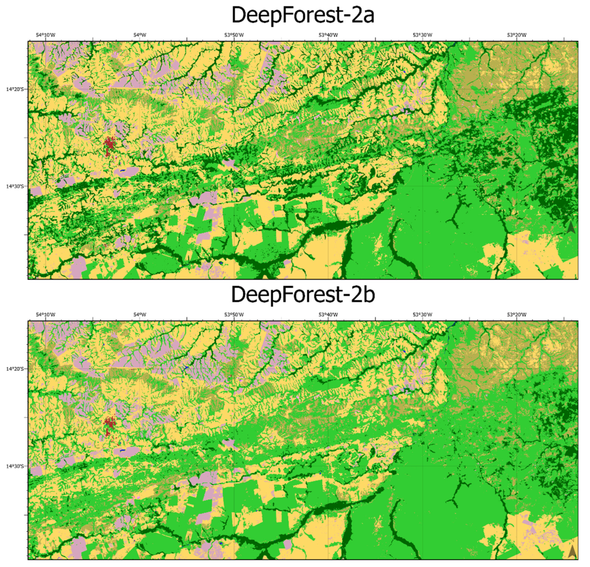
3.4. Qualitative Assessment

For the qualitative assessment, all models acting on the combined dataset (S1TsS2) were integrated into an ArcGIS Toolbox (GUI) to perform inference with a larger contiguous extent. We visually inspected the resulting maps and compared them to the MapBiomas Collection 4 labels from 2018 (shown in Figure 7).

Both SotA networks performed vastly differently with the dataset. The map produced by DeepLab (cf. Figure 8) looked visually similar to the labels of the MapBiomas project. Finer structures in areas with multiple classes were lost, while large contiguous areas of one class were correctly assigned. Additionally, some kind of tiling was clearly visible (i.e., northeast of the urban area) where classes exhibited hard edges that were horizontal or vertical. This effect was probably caused by the tiling of the dataset along the x-y-plane.

The map produced by U-Net (see Figure 8) showed major misclassifications of the urban infrastructure class, as well as grassland formations. The tiling effect caused by the image tiles was not apparent in this classification. Overall, this model did not seem to be able to produce reliable results with multi-modal input data.

Both predicted maps appeared smoother compared to the salt and pepper effect of the labels. This was due to the pixel-based nature of the algorithms used to derive the label maps in the first place. CNNs, on the other hand, also consider the neighborhood and were capable of deriving information that was more coherent.

The three presented models using the early fusion approach, DeepForest-1a/b/c, produced visually similar maps, as shown in Figure 9. As in the SotA models, smoother maps were produced, with larger homogenous areas due to the spatial neighborhood considered by the classifiers. The tiling effect present in the map produced by DeepLab was also visible in the classifications of DeepForest-1a and -1c. They all showed the edge along 54°W east of the urban settlement. DeepForest-1b provided a more detailed classification of forest formation (dark green). It was the only model out of the three to detect some of the other non-vegetated areas (pink; between 53°50′W and 53°30′W).

The two representation-fusion models, DeepForest-2a and -2b, showed more fine-grained classifications compared to the other models (cf. Figure 10). As in the MapBiomas label map, these models produced less homogenous large patches. None of the tiling artifacts from the other models were present here. However, structures such as the river in the northeastern part of the extent were not present in the classification maps of either of these models. They also seemed to omit the other non-vegetated area class completely. The classification of the urban area visible in the maps seemed to be more concise with the labels.

4. Discussion

In a realm of dynamic land cover and challenging weather conditions for optical remote sensing data, we proposed new deep learning models employing two different data fusion approaches—namely, early and representation fusion—for LULC assessment in the Amazon forest. We addressed several design and conceptual aspects of computer vision DL models and adapted them for remote sensing data. The results of multiple experiments highlighted the potential of these DL architectures with multi-modal data. However, many uncertainties and challenges were involved in the process and need to be taken into consideration to produce robust and reliable models with new data. In the following, we discuss the opportunities and the challenges of the presented approaches and the quality of our results compared to similar studies. A direct comparison, however, is difficult due to the differences in the application, number and kind of classes, the sensors used and the challenges of weakly supervised learning.

4.1. Effect of the Synergy between Sentinel-1 and Sentinel-2 Data

The synergetic use of Sentinel-1 and Sentinel-2 data indeed improved the land cover mapping capability in the context of weakly supervised learning. This might be counter-intuitive since the best OA accuracy of 77.9% was achieved with mono-modal data (Table 3). However, this was due to the high bias of OA towards the dominant class (FF) covering 43% of the area. Compared to the mono-modal experiments (S2), the multi-modal approaches showed an improvement in mapping some complex and underrepresented land cover classes, except for the U-Net model (cf. Table 3 and Table 4). For instance, classification of savanna can be challenging, as this class can be confused with forest, grassland and pasture (cf. Figure 6) [44]. Therefore, this class is often omitted from analyses [26]. From the confusion matrices of the best-performing models with S2 (U-Net) vs. S1TsS2_12 (DeepLab) in Figure 6 (also see Figure A1), we can note a decrease in the false predictions of savanna from grassland and pasture. This can be explained partly by the use of ASPP but also by the features introduced with SAR data.

Furthermore, by using time-series SAR data, some models were able to better classify the annual and perennial crops (cf. Table 3 and Table 4), as most models showed significant improvements in F1 and IoU. Time-series scenes can capture the different plant phenologies during the crop life cycle, from seedlings to fully developed crops. For example, soybeans are fully ripe in southern Brazil in March [45], while the harvesting season for corn already begins in January [46].

Shortening the time-series length did not show a significant change in the results. Although using few bands can be beneficial to save computational resources, it requires specific consideration of the involved classes and the nature of the area of interest since some land cover can benefit from shorter time spans while others might not be captured well.

4.2. Classification Scheme and Label Quality

The experiments implemented with weak labels showed promising results. The models were able to learn the important features for the dominant classes and even improve the delivered representation maps (cf. Figure 9 and Figure 10). However, for LULC classification, it is difficult to obtain error-free labels, especially in a very dynamic environment such as the Amazon [19]. In contrast to the existing benchmark datasets with controlled quality of labels (e.g., SEN12MS [26]), it is challenging to evaluate the quality of the results from real-world datasets. Low accuracies can be induced from either misclassification errors or mislabeling. Additionally, due to resource limitations, it was not possible to test the models with the same large extent. This had an impact on the difference in the class distribution (different proportions for the class imbalance) and, therefore, on the models’ performance. Due to the strong class imbalance, the technique applied to circumvent this issue (weighted loss functions) did not result in any remarkable improvement in the results. To efficiently solve this problem, a prior sampling process of the area of extent is recommended [47].

Another main issue with LULC studies is appropriately defining the classification scheme. As this is very application domain-related, it is difficult to agree on a global scheme, given the heterogeneity of available label sources [48]. This is one of the limitations in this study, and we acknowledge that the classification scheme adopted in the ground-truth data had a significant effect on the quality of the model results. A suggestion for improvement is to use more generic classes based on the properties of the area or the research questions addressed.

4.3. Discussion of the Results Compared to Related Studies

The results of the present study show that classification of LULC demonstrated good overall results using SotA methods applied to single-date multi-spectral data (S2). However, the inclusion of Sentinel-1 time-series improved the classification, especially considering underrepresented classes.

In a case study in the tropical forests of Myanmar, the authors of [49] used a combination of Landsat imagery and L-Band SAR data (JERS-1 and ALOS-2/PALSAR-2) to classify nine classes using an RF algorithm. Although this study used single-date imagery instead of SAR time-series, the authors showed an increase in classification accuracy when using multi-modal data.

An improvement in classification results due to spatiotemporal data fusion was also shown in another study [50]. The authors compared six spatiotemporal deep learning models, including ConvLSTM, which is one of the building blocks of DeepForest. They used a series of median composite Landsat images from across the tropics to classify seven follow-up land use classes after deforestation. The ConvLSTM model was among the best in all tropical areas. However, the authors mainly showed that the classification performance, measured as the class-wise F1 score, was very dependent on location. Combing multiple seemingly similar regions into one training set vastly reduces accuracy and highlights the importance of regional differences in vegetation that might hamper automation on a very large scale, such as the whole Amazon basin. This regional consideration is taken into account in the MapBiomas project [19], which uses different models and learning strategies for different biomes of Brazil.

Another study in Brazil [51] used a time-series of 42 Sentinel-1 scenes combined with a mosaic of Seninel-2 scenes in Paragominas. The authors also faced the problem of heavy cloud cover in this region, thus being unable to produce a time-series for the multi-spectral data. Their reference data were captured during a field mission, beating our labels in terms of quality and correctness. They defined seven major LULC classes for classification with an RF classifier. In contrast to our findings, they showed that the choice of the intra-annual time period of the SAR time series did not play a significant role. However, our approach used much more computationally intensive and dynamic models; thus, we argue that a good choice of time period for inclusion in the training process is important, as we experienced an increase in classification performance. This could save on costly computation time in the learning and inference process due to dropping data from time periods that do not significantly contribute to the model performance.

The authors of [52] used time-series for both the multi-spectral Sentinel-2 images and the Sentinel-1 data. This represents the most comparable setting to our study with respect to data fusion. They compared RF [13], ConvLSTM [41] and their own proposed dual-stream CNN combined with an RNN architecture called TWINNS. They trained these models on data from Burkina Faso and Reunion with 8 and 13 classes, respectively. In Burkina Faso, the model could achieve at most an OA of 87.5%, and it achieved 89.97% in Reunion. However, the ground truth was mostly captured by labor-intensive in situ measurements and expert interpretation of VHR imagery and, therefore, the problems with weakly supervised learning were not relevant for their study. This is not feasible for most areas and, therefore, not directly comparable to our study. However, this comparison highlights that good labels are crucial for good results. Furthermore, the investigation of how to deal with weakly supervised learning is very important and the issue could be tackled by, for example, a combination of unsupervised and supervised learning approaches.

5. Conclusions

Due to the challenging weather conditions in the Amazon basin, using multi-modal remote sensing data is a compelling approach to improve LULC classification. In the present study, we compared different fusion approaches using DL, including spatiotemporal aspects, and propose novel deep learning approaches.

Our results highlight improvements in detecting underrepresented LULC classes, with additional spectral similarities to other dominating classes when using the proposed novel deep learning approaches. The potential of developing DL models specifically for multi-modal and multi-temporal satellite data for large-scale mapping in tropical regions is clearly shown by our results. Furthermore, the integration of the novel models within a GUI is of great importance for potential users who might not be familiar with coding. We used the inference function on a larger area to conduct qualitative assessment of the results, which shows that quantitative results might sometimes be misleading, especially in the presence of class imbalances and inaccurate labels.

More research is needed to explore better methods for dealing with inaccurate and noisy label data. Ongoing research is diving into the employment of methods to cluster robust labels, such as self-supervision techniques [53,54], on even larger datasets from the Amazon area and will hopefully further improve large-scale mapping of this highly important environment.

References

1. The World Bank New Project to Implement Sustainable Landscapes in the Brazilian Amazon. Available online: https://www.worldbank.org/en/news/press-release/2017/12/14/brazil-amazon-new-project-implement-sustainable-landscapes (accessed on 21 May 2022).
2. Pulella, A.; Aragão Santos, R.; Sica, F.; Posovszky, P.; Rizzoli, P. Multi-Temporal Sentinel-1 Backscatter and Coherence for Rainforest Mapping. Remote Sens. 2020, 12, 847. [Google Scholar] [CrossRef] [Green Version]
3. Carreiras, J.M.B.; Jones, J.; Lucas, R.M.; Shimabukuro, Y.E. Mapping Major Land Cover Types and Retrieving the Age of Secondary Forests in the Brazilian Amazon by Combining Single-Date Optical and Radar Remote Sensing Data. Remote Sens. Environ. 2017, 194, 16–32. [Google Scholar] [CrossRef] [Green Version]
4. Le Quéré, C.; Capstick, S.; Corner, A.; Cutting, D.; Johnson, M.; Minns, A.; Schroeder, H.; Walker-Springett, K.; Whitmarsh, L.; Wood, R. Towards a Culture of Low-Carbon Research for the 21st Century. Tyndall Cent. Clim. Chang. Res. Work. Pap. 2015, 161, 1–25. [Google Scholar]
5. Heckenberger, M.J.; Christian Russell, J.; Toney, J.R.; Schmidt, M.J. The Legacy of Cultural Landscapes in the Brazilian Amazon: Implications for Biodiversity. Phil. Trans. R. Soc. B 2007, 362, 197–208. [Google Scholar] [CrossRef] [Green Version]
6. The Nature Conservancy The Amazon Is Our Planet’s Greatest Life Reserve and Our World’s Largest Tropical Rainforest. Available online: https://www.nature.org/en-us/get-involved/how-to-help/places-we-protect/amazon-rainforest/ (accessed on 18 February 2022).
7. PRODES—Coordenação-Geral de Observação Da Terra. Available online: http://www.obt.inpe.br/OBT/assuntos/programas/amazonia/prodes/prodes/ (accessed on 10 December 2021).
8. Marschner, F.J.; Anderson, J.R. Major Land Uses in the United States; U.S. Geological Survey: Reston, VA, USA, 1967; pp. 158–159. Available online: https://pubs.er.usgs.gov/publication/70046790 (accessed on 10 December 2021).
9. Vali, A.; Comai, S.; Matteucci, M. Deep Learning for Land Use and Land Cover Classification Based on Hyperspectral and Multispectral Earth Observation Data: A Review. Remote Sens. 2020, 12, 2495. [Google Scholar] [CrossRef]
10. Nasrallah, A.; Baghdadi, N.; El Hajj, M.; Darwish, T.; Belhouchette, H.; Faour, G.; Darwich, S.; Mhawej, M. Sentinel-1 Data for Winter Wheat Phenology Monitoring and Mapping. Remote Sens. 2019, 11, 2228. [Google Scholar] [CrossRef] [Green Version]
11. Sica, F.; Pulella, A.; Nannini, M.; Pinheiro, M.; Rizzoli, P. Repeat-Pass SAR Interferometry for Land Cover Classification: A Methodology Using Sentinel-1 Short-Time-Series. Remote Sens. Environ. 2019, 232, 111277. [Google Scholar] [CrossRef]
12. Colditz, R.R. An Evaluation of Different Training Sample Allocation Schemes for Discrete and Continuous Land Cover Classification Using Decision Tree-Based Algorithms. Remote Sens. 2015, 7, 9655–9681. [Google Scholar] [CrossRef] [Green Version]
13. Breiman, L. Random Forests. Mach. Learn. 2001, 45, 5–32. [Google Scholar] [CrossRef] [Green Version]
14. Mountrakis, G.; Im, J.; Ogole, C. Support Vector Machines in Remote Sensing: A Review. ISPRS J. Photogramm. Remote Sens. 2011, 66, 247–259. [Google Scholar] [CrossRef]
15. Belgiu, M.; Drăguţ, L. Random Forest in Remote Sensing: A Review of Applications and Future Directions. ISPRS J. Photogramm. Remote Sens. 2016, 114, 24–31. [Google Scholar] [CrossRef]
16. Mapbiomas Brasil. Available online: https://mapbiomas.org/en (accessed on 17 March 2022).
17. Steinhausen, M.J.; Wagner, P.D.; Narasimhan, B.; Waske, B. Combining Sentinel-1 and Sentinel-2 Data for Improved Land Use and Land Cover Mapping of Monsoon Regions. Int. J. Appl. Earth Obs. Geoinf. 2018, 73, 595–604. [Google Scholar] [CrossRef]
18. Foerster, S.; Kaden, K.; Foerster, M.; Itzerott, S. Crop Type Mapping Using Spectral–Temporal Profiles and Phenological Information. Comput. Electron. Agric. 2012, 89, 30–40. [Google Scholar] [CrossRef] [Green Version]
19. Souza, J.; Siqueira, J.V.; Sales, M.H.; Fonseca, A.V.; Ribeiro, J.G.; Numata, I.; Cochrane, M.A.; Barber, C.P.; Roberts, D.A.; Barlow, J. Ten-Year Landsat Classification of Deforestation and Forest Degradation in the Brazilian Amazon. Remote Sens. 2013, 5, 5493–5513. [Google Scholar] [CrossRef] [Green Version]
20. LeCun, Y.; Bengio, Y. Convolutional Networks for Images, Speech, and Time Series. In The Handbook of Brain Theory and Neural Networks; MIT Press: Cambridge, MA, USA, 1998; pp. 255–258. ISBN 978-0-262-51102-5. [Google Scholar]
21. Zhu, X.X.; Tuia, D.; Mou, L.; Xia, G.-S.; Zhang, L.; Xu, F.; Fraundorfer, F. Deep Learning in Remote Sensing: A Comprehensive Review and List of Resources. IEEE Geosci. Remote Sens. Mag. 2017, 5, 8–36. [Google Scholar] [CrossRef] [Green Version]
22. Ball, J.E.; Anderson, D.T.; Sr, C.S.C. Comprehensive Survey of Deep Learning in Remote Sensing: Theories, Tools, and Challenges for the Community. J. Appl. Remote Sens. 2017, 11, 042609. [Google Scholar] [CrossRef] [Green Version]
23. Yuan, X.; Shi, J.; Gu, L. A Review of Deep Learning Methods for Semantic Segmentation of Remote Sensing Imagery. Expert Syst. Appl. 2021, 169, 114417. [Google Scholar] [CrossRef]
24. Mahdianpari, M.; Salehi, B.; Rezaee, M.; Mohammadimanesh, F.; Zhang, Y. Very Deep Convolutional Neural Networks for Complex Land Cover Mapping Using Multispectral Remote Sensing Imagery. Remote Sens. 2018, 10, 1119. [Google Scholar] [CrossRef] [Green Version]
25. Schmitt, M.; Prexl, J.; Ebel, P.; Liebel, L.; Zhu, X.X. Weakly Supervised Semantic Segmentation of Satellite Images for Land Cover Mapping—Challenges and Opportunities. arXiv 2020, arXiv:2002.08254. [Google Scholar] [CrossRef]
26. Schmitt, M.; Hughes, L.H.; Qiu, C.; Zhu, X.X. SEN12MS—A Curated Dataset of Georeferenced Multi-Spectral Sentinel-1/2 Imagery for Deep Learning and Data Fusion. arXiv 2019, arXiv:1906.07789. [Google Scholar] [CrossRef] [Green Version]
27. Loveland, T.R.; Belward, A.S. The IGBP-DIS Global 1km Land Cover Data Set, DISCover: First Results. Int. J. Remote Sens. 1997, 18, 3289–3295. [Google Scholar] [CrossRef]
28. Neves, A.K.; Körting, T.S.; Fonseca, L.M.G.; Girolamo Neto, C.D.; Wittich, D.; Costa, G.A.O.P.; Heipke, C. Semantic segmentation of Brazilian savanna vegetation using high spatial resolution satellite data and U-net. ISPRS Ann. Photogramm. Remote Sens. Spat. Inf. Sci. 2020, 5, 505–511. [Google Scholar] [CrossRef]
29. Espinoza Villar, J.C.; Ronchail, J.; Guyot, J.L.; Cochonneau, G.; Naziano, F.; Lavado, W.; De Oliveira, E.; Pombosa, R.; Vauchel, P. Spatio-Temporal Rainfall Variability in the Amazon Basin Countries (Brazil, Peru, Bolivia, Colombia, and Ecuador). Int. J. Climatol. 2009, 29, 1574–1594. [Google Scholar] [CrossRef] [Green Version]
30. Arvor, D.; Funatsu, B.M.; Michot, V.; Dubreuil, V. Monitoring Rainfall Patterns in the Southern Amazon with PERSIANN-CDR Data: Long-Term Characteristics and Trends. Remote Sens. 2017, 9, 889. [Google Scholar] [CrossRef] [Green Version]
31. Peterson, J. Rainforest Weather & Climate. Available online: https://sciencing.com/rainforest-weather-climate-19521.html (accessed on 14 August 2022).
32. JEC Assessment: Mato Grosso. 2021. Available online: https://www.andgreen.fund/wp-content/uploads/2022/02/JECA-Mato-Grosso-Full_compressed.pdf (accessed on 8 November 2021).
33. Yale University. The Amazon Basin Forest | Global Forest Atlas. Available online: https://web.archive.org/web/20190630052510/https://globalforestatlas.yale.edu/region/amazon (accessed on 20 September 2022).
34. Souza, C.M.; Azevedo, T. ATBD_R Algorithm Theoretical Base Document & Results. In MapBiomas General “Handbook”; MapBiomas: São Paulo, Brazil, 2017; Volume 24. [Google Scholar] [CrossRef]
35. Zhou, Z.-H. A Brief Introduction to Weakly Supervised Learning. Natl. Sci. Rev. 2018, 5, 44–53. [Google Scholar] [CrossRef] [Green Version]
36. Ronneberger, O.; Fischer, P.; Brox, T. U-Net: Convolutional Networks for Biomedical Image Segmentation. In Proceedings of the International Conference on Medical Image Computing and Computer-Assisted Intervention, Munich, Germany, 5–9 October 2015; pp. 234–241. [Google Scholar]
37. Chen, L.-C.; Papandreou, G.; Kokkinos, I.; Murphy, K.; Yuille, A.L. DeepLab: Semantic Image Segmentation with Deep Convolutional Nets, Atrous Convolution, and Fully Connected CRFs. IEEE Trans. Pattern Anal. Mach. Intell. 2018, 40, 834–848. [Google Scholar] [CrossRef] [Green Version]
38. Long, J.; Shelhamer, E.; Darrell, T. Fully Convolutional Networks for Semantic Segmentation. In Proceedings of the IEEE Conference on Computer Vision and Pattern Recognition, Boston, MA, USA, 7–12 June 2015; pp. 3431–3440. [Google Scholar]
39. Scharvogel, D.; Brandmeier, M.; Weis, M. A Deep Learning Approach for Calamity Assessment Using Sentinel-2 Data. Forests 2020, 11, 1239. [Google Scholar] [CrossRef]
40. He, K.; Zhang, X.; Ren, S.; Sun, J. Deep Residual Learning for Image Recognition. In Proceedings of the IEEE Conference on Computer Vision and Pattern Recognition, Las Vegas, NV, USA, 27–30 June 2016; pp. 770–778. [Google Scholar] [CrossRef] [Green Version]
41. Shi, X.; Chen, Z.; Wang, H.; Yeung, D.-Y.; Wong, W.; Woo, W. Convolutional LSTM Network: A Machine Learning Approach for Precipitation Nowcasting. Adv. Neural Inf. Process. Syst. 2015, 28, 9. [Google Scholar]
42. Ioffe, S.; Szegedy, C. Batch Normalization: Accelerating Deep Network Training by Reducing Internal Covariate Shift. In Proceedings of the International Conference on Machine Learning, Lille, France, 6–11 June 2015; pp. 448–456. [Google Scholar]
43. Hochreiter, S.; Schmidhuber, J. Long Short-Term Memory. Neural Comput. 1997, 9, 1735–1780. [Google Scholar] [CrossRef]
44. Alencar, A.; Shimbo, J.Z.; Lenti, F.; Balzani Marques, C.; Zimbres, B.; Rosa, M.; Arruda, V.; Castro, I.; Fernandes Márcico Ribeiro, J.P.; Varela, V.; et al. Mapping Three Decades of Changes in the Brazilian Savanna Native Vegetation Using Landsat Data Processed in the Google Earth Engine Platform. Remote Sens. 2020, 12, 924. [Google Scholar] [CrossRef]
45. Costa, O.B.d.; Matricardi, E.A.T.; Pedlowski, M.A.; Cochrane, M.A.; Fernandes, L.C. Spatiotemporal Mapping of Soybean Plantations in Rondônia, Western Brazilian Amazon. Acta Amaz. 2017, 47, 29–38. [Google Scholar] [CrossRef] [Green Version]
46. Becker, W.R.; Richetti, J.; Mercante, E.; Esquerdo, J.C.D.M.; da Silva Junior, C.A.; Paludo, A.; Johann, J.A. Agricultural Soybean and Corn Calendar Based on Moderate Resolution Satellite Images for Southern Brazil. Semin. Cienc. Agrar. 2020, 41, 2419–2428. [Google Scholar] [CrossRef]
47. Susan, S.; Kumar, A. The Balancing Trick: Optimized Sampling of Imbalanced Datasets—A Brief Survey of the Recent State of the Art. Eng. Rep. 2021, 3, e12298. [Google Scholar] [CrossRef]
48. Tulbure, M.G.; Hostert, P.; Kuemmerle, T.; Broich, M. Regional Matters: On the Usefulness of Regional Land-Cover Datasets in Times of Global Change. Remote Sens. Ecol. Conserv. 2022, 8, 272–283. [Google Scholar] [CrossRef]
49. De Alban, J.D.T.; Connette, G.M.; Oswald, P.; Webb, E.L. Combined Landsat and L-Band SAR Data Improves Land Cover Classification and Change Detection in Dynamic Tropical Landscapes. Remote Sens. 2018, 10, 306. [Google Scholar] [CrossRef] [Green Version]
50. Masolele, R.N.; De Sy, V.; Herold, M.; Marcos, D.; Verbesselt, J.; Gieseke, F.; Mullissa, A.G.; Martius, C. Spatial and Temporal Deep Learning Methods for Deriving Land-Use Following Deforestation: A Pan-Tropical Case Study Using Landsat Time Series. Remote Sens. Environ. 2021, 264, 112600. [Google Scholar] [CrossRef]
51. Mercier, A.; Betbeder, J.; Rumiano, F.; Baudry, J.; Gond, V.; Blanc, L.; Bourgoin, C.; Cornu, G.; Ciudad, C.; Marchamalo, M.; et al. Evaluation of Sentinel-1 and 2 Time Series for Land Cover Classification of Forest–Agriculture Mosaics in Temperate and Tropical Landscapes. Remote Sens. 2019, 11, 979. [Google Scholar] [CrossRef] [Green Version]
52. Ienco, D.; Interdonato, R.; Gaetano, R.; Ho Tong Minh, D. Combining Sentinel-1 and Sentinel-2 Satellite Image Time Series for Land Cover Mapping via a Multi-Source Deep Learning Architecture. ISPRS J. Photogramm. Remote Sens. 2019, 158, 11–22. [Google Scholar] [CrossRef]
53. Wang, Y.; Albrecht, C.; Ait Ali Braham, N.; Mou, L.; Zhu, X. Self-Supervised Learning in Remote Sensing: A Review. IEEE Geosci. Remote Sens. Mag. 2022, 15, 2–36. [Google Scholar] [CrossRef]
54. Xue, Z.; Yu, X.; Yu, A.; Liu, B.; Zhang, P.; Wu, S. Self-Supervised Feature Learning for Multimodal Remote Sensing Image Land Cover Classification. IEEE Trans. Geosci. Remote Sens. 2022, 60, 1–15. [Google Scholar] [CrossRef]
Figure 1. The global workflow of the LULC classification process with the tools and technologies used at each step.
Remotesensing 14 05000 g001
Figure 2. Sentinel-2 scenes (green bounding boxes) and the areas of interest (AOIs) for the combined Sentinel-1 time-series + Sentinel-2 data (red bounding box) used in this study.
Remotesensing 14 05000 g002
Figure 3. Pre-processing chain for Sentinel-1 data performed in SNAP.
Remotesensing 14 05000 g003
Figure 4. DeepForest variations: (a) DeepForest architecture with one ConvLSTM block (DeepForest-1a). (b) DeepForest architecture with two ConvLSTM blocks (DeepForest-1b). (c) DeepForest with an ASPP block (DeepForest-1c).
Remotesensing 14 05000 g004
Figure 5. The architecture of the two-branch model DeepForest-2. For the multispectral stream, a prior learned classifier was used; i.e., DeepLab or one of the DeepForest-1 model variations.
Remotesensing 14 05000 g005
Figure 6. Confusion matrices for the best-performing model with mono-modal data ((a): U-Net) vs. multi-modal data ((b): DeepLab).
Remotesensing 14 05000 g006
Figure 7. Map showing the MapBiomas Collection 4 labels from 2018. This extent was used for the qualitative assessment. Legend colors were chosen to be coherent with the MapBiomas Project.
Remotesensing 14 05000 g007
Figure 8. Classification maps using the SotA networks DeepLab and U-Net. The legend for these is presented in Figure 8.
Remotesensing 14 05000 g008
Figure 9. Classification maps produced with the presented early fusion models DeepForest-1a/b/c. The legend for these maps is presented in Figure 8.
Remotesensing 14 05000 g009
Figure 10. Classification maps produced with the presented representation fusion models DeepForest-2a/b. The legend for these maps is presented in Figure 8.
Remotesensing 14 05000 g010