Daily Spatial Distribution of Apparent Temperature Comfort Zone in China Based on Heat Index

Abstract

Apparent temperature (AT) is used to evaluate human comfort and is of great importance for studies on the effects of environmental factors on human health. This study used the daytime heat index (HI) calculated by national surface meteorological stations in China as the AT dependent variable, with August 2020 employed as an example. The daytime fifth generation European Centre for Medium-Range Weather Forecasts (ECMWF) atmospheric reanalysis of the global climate (ERA5) data and multi-source data extracted from the stations were used as the independent variables. Due to the presence of multicollinearity among the independent variables, we implemented a multiple stepwise regression model and developed a daily near-surface 1 km HI estimation model. The correlation analysis using the model showed that the coefficient of determination (R²) was 0.89; the mean absolute error (MAE) was 1.49 °C, and the root mean square error (RMSE) was 2.08 °C. We also used 10-fold cross-validation to calculate the error between the parameter and predicted values. The R² of the model was 0.96; the MAE was 1.80 °C, and the RMSE was 2.40 °C. In this month, the mean daily daytime HI was 20.51 °C. According to the Universal Thermal Climate Index (UTCI), the areas with more than 20 days of heat stress for one month were largely distributed in the desert areas of northwest China and the coastal areas in southeast China, accounting for 29.98% of the total land area of China. This study improves the spatial resolution and accuracy of HI prediction, thus providing a scientific reference for studying residential environments and the urban heat island effect.

1. Introduction

With the rapid expansion of urbanized areas, the effects of environmental factors on human health have attracted increasing concern [1]. In the natural environment, the temperature is the main factor that affects human comfort, and temperature changes will result in body temperature adjustment behaviors and heart rate changes that can cause heart-head blood vessel disease [2]. The associated changes in humidity and wind speed [3,4] affect human metabolism, thereby increasing the susceptibility to disease [3,5,6]. Apparent temperature (AT), first proposed by Steadman in 1971 [7], is used to evaluate the perception of exposed body surface under cold and windy conditions [8]. It is affected by temperature, humidity, wind speed, and other factors [9,10] and is an intuitive reflection of the degree of warmth of the external environment. Many studies have been conducted on “short-term” extreme climate events, but few studies have focused on the effects of chronic exposure. Previous studies have indicated that exposure to uncomfortable environments for a long period of time will affect health services, increase accident risk, increase disease risk, restrict worker productivity, health and wellbeing, and affect urban GDP and economic development [11]. The AT is more suitable for spatial epidemiological studies [7,12,13,14,15,16]. We aimed to explore the effects of long-term heat stress on residents’ health on a daily scale.

Many methods for AT calculation have been proposed, and studies have been conducted worldwide, primarily empirical studies and those employing mechanistic models. Most such studies have been based on empirical models [17]. For example, Li et al. explored the relationship between the number of deaths and AT changes by adjusting the degrees of freedom of AT-influencing factors in a generalized additive model (GAM) [18,19]. Wang et al. proposed a calculation method for human comfort based on the golden section method that included latitude, altitude, season, and other aspects, and they formulated an optimal calculation for human comfort [20]. In the climate suitability evaluation method of China’s industry-standard summer tourism, only the daily maximum and minimum temperatures, daily average relative humidity, and daily average wind speed are considered when calculating the AT [21,22]. In establishing an AT model based on heat balance, Liu et al. found that radiation was the only source of energy that the human body obtained from the environment. Still, net radiation plays an important role [23]. Zhu et al. found that in the absence of direct sunlight, the radiation exchange between the human body and the environment is balanced, and thus has little effect on heat dissipation in the human body. Under general weather conditions, we can give priority to temperature and humidity [24]. Steadman divided the application range of the AT based on actual conditions in Australia and connected this to a standard scale [9,25]. Masterton and Richardson of the Canadian Atmospheric Environment Agency proposed that the humidity index (humidex) and heat index (HI), where the former is based on air and dewpoint temperatures [26], have significant effects [27]. Other researchers have combined the AT and humidex. Furthermore, the AT has shown good applicability in heat wave research [28], but has had low spatial resolution. Moreover, these simple empirical indices only consider some relevant meteorological parameters and do not account for thermal physiology [29].

Compared to the empirical models, the mechanistic models comprehensively consider environmental factors such as human metabolic respiratory heat dissipation and clothing thermal resistance, and thus are better for calculating human comfort [30]. Fanger, a Danish researcher, published a thermal comfort equation in 1970 that proposed three conditions for satisfying human comfort and creatively combined the heat balance model with human biometrics [16]. Accordingly, the concept of skin moisture was introduced, and the effective temperature (ET), standard ET (SET) [31], and physiological equivalent temperature (PET) were proposed [32]. In 1979, Steadman proposed the HI calculated from the temperature and relative humidity, including assumptions of human mass, height, clothing, physical activity, individual heat tolerance, exposure to sunlight and ultraviolet radiation, and wind speed [9]. This index is often used to represent the perceived body temperature. Rothfusz modified the HI in 1990, and this definition is currently used by the National Weather Service (NWS) [33]. However, data employed by the mechanistic models, such as metabolic respiratory heat dissipation and clothing thermal resistance, are difficult to obtain and apply in this research area.

Empirical and mechanistic models are primarily based on on-site meteorological observations and do not provide spatial details regarding urban thermal comfort. The ability of remote sensing to describe spatial details and physical processes has been continuously improved, providing an excellent opportunity for enhancing our understanding of the urban thermal environment on a fine spatial-temporal scale [34]. How to realize high-precision climate comfort prediction in a large space by remote sensing will become increasingly meaningful. At present, the commonly used prediction models include machine learning, multiple linear regression models, and derived models. Machine learning techniques such as RF/BT are widely used and have good application in calculating the importance of variables based on the interactions between variables. Multiple stepwise regression models are established based on the importance and relevance of independent variables to the heat index, a common method to eliminate multicollinearity [35]. We selected the commonly used methods, including multiple stepwise regression models and multiple linear regression models, in the present study. We used the modified HI calculation method to obtain the daytime HI as the daily HI of China from meteorological stations. We defined the daytime as 6 am to 6 pm (UTC/GMT + 08:00) and selected August 2020 as the research period, as it is typically the hottest month of the year. Owing to the discontinuous spatial distribution of meteorological stations, this study used atmospheric reanalysis data to replace the corresponding station data. The data incorporated the normalized vegetation index (NDVI) [36,37,38,39], the normalized water index (NDWI) [40], the night light index (NTL), and elevation. We established a multivariate stepwise regression model to screen the independent variables and build a multivariate linear regression model for HI prediction. The predicted results were compared to the HI from the meteorological stations. HI distribution characteristics had a resolution of 1 km in the study area. We calculated the duration and area change in the heat stress area. By combining the atmospheric reanalysis data and multi-source data, we accounted for the shortcomings of the discontinuous spatial distribution of the meteorological stations, thereby improving the accuracy of predictions of the spatial distribution of the regional HI.

2. Materials and Methods

2.1. Study Area

China is located in East Asia and along the west coast of the Pacific Ocean. The terrain is high in the west, low in the east, and harbors complex and diverse climate types. The east has a monsoon climate, the northwest has a temperate continental climate, and the Qinghai-Tibet Plateau has an alpine climate. The complexity and diversity of the terrain and climate affect the apparent temperature and comfort of people’s work and life. Therefore, it is essential to predict AT changes accurately.

2.2. Meteorological Station Data

Data acquired by China’s national surface meteorological stations have high precision but are not continuous in space. The atmospheric reanalysis data are continuous in space, but their spatial resolution is low. By combining multi-source data and using the surface meteorological station data for verification, we obtained HI distribution characteristics high in precision and resolution. We selected global hourly data from the national meteorological stations in China from the National Environmental Information Center (NCEI) (https://www.ncei.noaa.gov/) (accessed on 1 April 2022). Based on the integrity of the station data, 376 national meteorological stations were selected, and the data records included the hourly air temperature, the dewpoint temperature, and other data from August 2020. As shown in Figure 1, the distribution of China’s national meteorological stations is relatively uniform and dispersed, representing a great deal of spatial resolution in the HI inversion process.

2.3. Multi-Source Data in the Heat Index Calculation

Air temperature is the main influencing factor on the HI, and its primary source is the solar radiation absorbed by the surface. Research has shown that communities with less vegetation and higher surface temperatures near the living environment are related to more deaths when residents are exposed to high temperatures [36,39,40]. The NDVI and NDWI have strong negative effects on the land surface temperature (LST) that can restrict the urban heat island effect and reduce the harm of heat stress [41,42]. Therefore, we considered adding the NDVI and NDWI to the heat index calculation. Meteorological conditions have the most direct effect on the HI. We selected the LST at 2 m, air temperature at 2 m (TEMP), dew point temperature (DEW) at 2 m, longitude wind speed at 10 m (WS_U), latitude wind speed at 10 m (WS_V), and atmospheric pressure (ATM) from the ECMWF ERA5-LAND HOURLY dataset for calculating the AT [43]. The selected period for records was 6 am to 6 pm. We calculated the U and V wind speeds obtained from ERA5 using the equation $\sqrt[2]{WS\text{\_}{U}^2+WS\text{\_}{V}^2}$ to obtain the actual wind speed (WS). To explore the effects of urban economic development level and population aggregation on human comfort, we incorporated NASA’s Black Marble VNP46A2 Daily Moonlight-adjusted Nighttime Lights (NTL) product into the calculation process [44]. The effects of altitude on temperature were apparent [45]. Therefore, ASTER GDEM 30 m resolution elevation data were added, as this was expected to improve the spatial resolution of the HI. The DEM elevation data were obtained from the third version of the product released in 2019. Their specific parameters are shown in

Table 1. Multi-source data used in the heat index calculation (links all accessed on 1 August 2022).

Data	Source	Links	Spatial Coverage	Horizontal Grid Spacing	Time Resolution
LST	ERA5_LAND HOURLY	https://cds.climate.copernicus.eu/	Global	0.1° ≈ 11.3 km	Daily
TEMP	ERA5_LAND HOURLY	https://cds.climate.copernicus.eu/	Global	0.1° ≈ 11.3 km	Daily
DEW	ERA5_LAND HOURLY	https://cds.climate.copernicus.eu/	Global	0.1° ≈ 11.3 km	Daily
ATM	ERA5_LAND HOURLY	https://cds.climate.copernicus.eu/	Global	0.1° ≈ 11.3 km	Daily
WS_U	ERA5_LAND HOURLY	https://cds.climate.copernicus.eu/	Global	0.1° ≈ 11.3 km	Daily
WS_V	ERA5_LAND HOURLY	https://cds.climate.copernicus.eu/	Global	0.1° ≈ 11.3 km	Daily
NDVI	MOD09GA	https://earthengine.google.com/	Global	463.3 m	Daily
NDWI	MOD09GA	https://earthengine.google.com/	Global	463.3 m	Daily
DEM	National Aeronautics and Space Administration	https://lpdaac.usgs.gov/products/astgtmv003/	Global	30 m	-
NTL	NASA’s Black Marble	https://blackmarble.gsfc.nasa.gov/	Global	500 m	Daily

.

All data selection times ranged from 6 am to 6 pm from 1 August to 31 August 2020. We calculated the average data of the selection times per day as the daily average data. Using the resample tool in ArcMap v10.6, atmospheric reanalysis data were resampled to a resolution of 1 km by bilinear interpolation. The DEM elevation data, NTL, NDVI, and NDWI were upscaled to produce coarser products with 1 km resolution [46], all of which adopted Lambert equiangular conic projection.

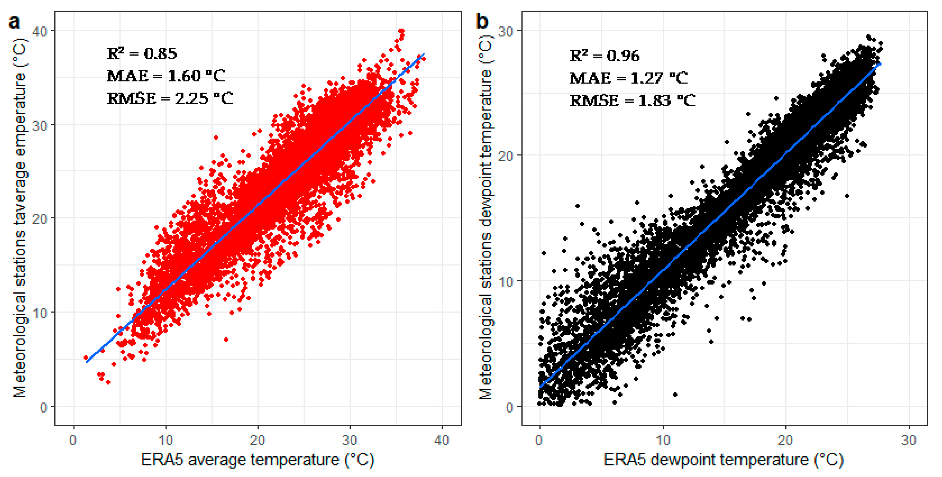
This study used atmospheric reanalysis data to retrieve the HI instead of meteorological station data. Their common data included the average temperature and dewpoint temperature. We analyzed the correlation between these measures by calculating the values of R², MAE, and RMSE. The analysis results are shown in Figure 2. The data were highly correlated, which provided a theoretical basis for our research.

2.4. Research Technical Route

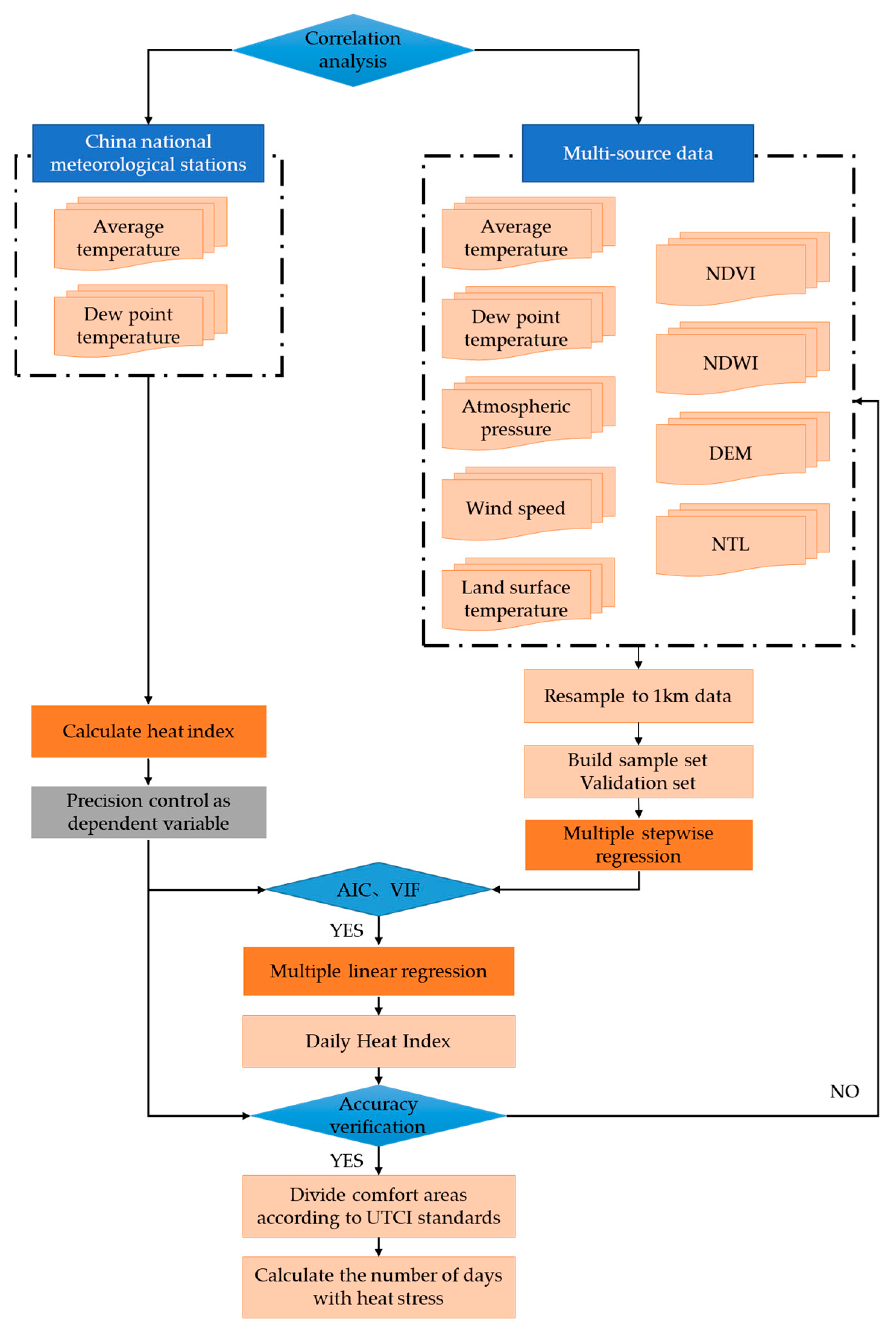
The technical route adopted in this study is shown in Figure 3. The specific steps were as follows:

(1)

Selection of multi-source data and pre-processing, and selection of meteorological factors that may potentially affect the HI. Pre-processing was implemented to unify the resolution and to coordinate the data system.

(2)

Selection of multi-source data obtained from the national surface meteorological stations in the study area, analysis of the correlation between data obtained from the meteorological station and atmospheric analysis, confirmation that the atmospheric reanalysis data can replace the meteorological station data, and finally the establishment of a multiple stepwise regression model. The optimal variables for the HI calculation were selected based on the Akaike information criterion (AIC) and variance inflation factor (VIF).

(3)

The HI calculated by the meteorological stations was used to verify the estimated HI calculated by the model. Calculation of the distribution characteristic diagram of the HI was conducted after the accuracy met the requirements. If the accuracy of the estimated HI model did not meet the requirements, the factors that potentially affected the HI were selected again, and the above steps were repeated.

(4)

According to the precision model calculation results, the HI distribution characteristics at a resolution of 1 km were calculated from the multi-source data using the ArcMap v10.6 grid computing tool. Based on the UTCI standard, the whole area was divided into 10 parts, and the duration days of area with heat stress were calculated.

2.5. HI

The HI is calculated from the air temperature and relative humidity; it is also known as the perceived air temperature (AT) and as the natural or perceived temperature. The HI makes assumptions concerning body mass, height, clothing, physical activity, individual heat resistance, exposure to sunlight and ultraviolet radiation, and wind speed. Significant deviations from these variables will not accurately reflect the HI value for perceived temperature. In 1979, Steadman proposed the HI as the AT, an index that is widely used in areas with hot conditions. Subsequently, we converted the calculated HI (℉) to °C [47]. The calculation formula is as follows [9]:

HI = 0.3564 × T + 0.0274104 × RH + 14.58824.

(1)

Rothfusz improved the calculation results of the HI in the technical annex (SR 90-23) of the NWS in 1990 [33]. We used this improved HI as the AT in this study, and its calculation formula is as follows [48]:

HI = −8.7847 + 1.6114 × T − 0.012308 × T² + RH × (2.3385 − 0.14612 × T) 2.2117 × 10⁻³ × T²) + RH² × (−0.016425 + 7.2546 × 10⁻⁴ × T − 3.582 × 10⁻⁶ × T²)

(2)

where HI is the heat index (°C); T is the average temperature (°C), and RH is the relative humidity (%).

Since there was no relative humidity in the daily data obtained from the meteorological stations and because HI is calculated from the air temperature and relative humidity, we used the average air temperature and DEW from the meteorological stations data to calculate the approximate value of the daily relative humidity. The following formula was used for the calculation [49]:

RH = 100 × (EXP ((17.625 × TD)/(243.04 + TD))/EXP ((17.625 × T)/(243.04 + T))),

(3)

where RH is the relative humidity, T is the average temperature (°C), and TD is the average DEW (°C).

2.6. Multiple Stepwise Regression Model

The basic idea of the stepwise regression was to reduce the degree of multicollinearity by removing variables that were less important and highly correlated with other variables. Variables were introduced into the model one by one. After each explanatory variable was introduced, F and t-tests were performed on the explanatory variables. When the introduced explanatory variables were no longer significant due to the introduction of subsequent explanatory variables, the original variables were deleted to ensure that only significant variables were included in the regression equation before each new variable was introduced. The final set of explanatory variables was considered optimal.

In this study, we used a forward selection method to establish a stepwise regression with the LST, TEMP, DEW, WS, ATM, NDVI, NDWI, NTL, and DEM data, selecting each variable based on its contribution to the heat index and retaining the statistically significant variables [50]. The HI of the surface meteorological stations was the dependent variable. We used k-fold cross-validation to divide the dataset randomly into two subparts, a training set and a testing set. The dataset was split into ‘k’ sub-samples, in which one sample was used for testing and the remaining k − 1 sub-samples were used for training purposes. After repeating k times by changing the training and testing datasets, the best model was selected by obtaining the minimum error based on various error estimation statistical tools [51,52]. Using the forward stepwise selection method, the AIC and VIF were used as evaluation indicators to find the HI inversion and best variable. The R², mean absolute error (MAE), and root mean square error (RMSE) values were used to calculate the error between the parameters and the prediction results. When the results of the AIC and VIF were optimal, we built the multivariate stepwise regression model as follows:

HI ~ a × LST + b × TEMP + c × DEW + d × WS
+ e × ATM + f × NDWI + g × NDVI + h × NTL + i × DEM + j,

(4)

where a, b, c, d, e, f, g, h, i, and j are the empirical coefficients calculated by the model; LST is the land surface temperature (°C); TEMP is the air temperature (°C); DEW is the dew point temperature (°C); WS is the actual wind speed (m/s); ATM is the atmospheric pressure (kPa); NDVI is the normalized vegetation index; NDWI is the normalized water index; NTL is the night light index (nW/cm²/sr), and DEM is the elevation (km). All significance tests satisfied p < 0.05.

The AIC measures the relative quality of statistical models using a given dataset. The criterion for measuring the fitting performance of the statistical model avoids overfitting to an extent [53]. The calculation formula of the AIC is as follows:

AIC = −2 ln (L) + 2k.

(5)

where L is the maximum likelihood under the model; k is the number of variables in the model.

The VIF measures the degree of multicollinearity between explanatory variables and other independent variables in the regression model to minimize the collinearity between independent variables [54]. The formula for calculating the VIF is as follows:

VIF = 1/(1 − R²),

(6)

where R² is the coefficient of determination.

2.7. Multiple Linear Regression Model

In practical problems, a phenomenon is often associated with multiple factors. The optimal combination of multiple independent variables for predicting or estimating the dependent variable is more effective and consistent than using only one independent variable for predictions or estimations.

The estimated monthly average HI calculated by the model was verified, and the R², MAE, and RMSE were used as accuracy evaluation indicators.

R² reflects the proportion of the total variance of the dependent variable that the independent variable can explain through a regression relationship. Its calculation formula is as follows:

$$R^2=1-\frac{{{\displaystyle \sum }}_i{\left({\widehat{y}}^{\left(i\right)}-y^{\left(i\right)}\right)}^2}{{{\displaystyle \sum }}_i{\left(\overline{y}-y^{\left(i\right)}\right)}^2}.$$

(7)

MAE is a measure of the mean absolute error between the predicted and true values. Its calculation formula is as follows:

$$MAE=\frac{1}{n} {{\displaystyle \sum }}_1^n\left|y_i-{\widehat{y}}_i\right|.$$

(8)

RMSE, based on the MSE, is the square root that measures the deviation between the observed and true values. It is often used as a measure of the prediction results of machine learning models. Its calculation formula is as follows:

$$RMSE=\sqrt[2]{\frac{1}{n}{{\displaystyle \sum }}_1^n{\left(y_i-{\widehat{y}}_i\right)}^2}.$$

(9)

where $y_i$ is the output variable; ${\widehat{y}}_i$ is the estimated value, and n is the total number of estimated values. Screening was conducted according to the contribution of each variable. Finally, the multiple regression equation for AT calculation was established.

2.8. Comfort Zone Division

The Universal Thermal Climate Index (UTCI) is a thermal index of the degree of human thermophysiological response based on research on human comfort by the World Meteorological Organization (WMO) Commission for Climatology [55]. It is commonly used to assess thermal stress in outdoor spaces, promote private and public health, develop appropriate urban planning, and study the effects of climatic conditions on heat stress. We used the equivalent temperature range generated by the UTCI for thermal stress to divide the daily comfort zone, as shown in

Table 2. The UTCI equivalent temperature classifies thermal stress.

UTCI Range (°C) 1	Stress Category	UTCI Range (°C)	Stress Category
>46	Extreme heat stress	0 to 9	Slight cold stress
38 to 46	Very strong heat stress	0 to −13	Moderate cold stress
32 to 38	Strong heat stress	−13 to −27	Strong cold stress
26 to 32	Moderate heat stress	−27 to −40	Very strong cold stress
9 to 26	No thermal stress	<−40	Extreme cold stress

¹ Temperature range (°C) corresponding to different thermal stress classifications.

[56].

3. Results

3.1. HI

3.1.1. HI Prediction

The sample set consisting of the LST, TEMP, DEW, WS, ATM, NDVI, NDWI, NTL, and DEM was screened. A total of 19,008 data points from 376 national surface meteorological stations in China in August 2020 were obtained. A daily multivariate stepwise regression model was constructed.

Table 3. Results of the multiple stepwise regression model.

	VARBALS *					R2	AIC	VIF	p-Value
1	+TEMP					0.86	52,004.48	1.00	<0.05
2	+TEMP	+DEW				0.88	50,013.95	1.52	<0.05
3	+TEMP	+DEW	−WS			0.89	49,628.11	1.65	<0.05
4	+TEMP	+DEW	−WS	−NDWI		0.89	49,322.25	1.80	<0.05
5	+TEMP	+DEW	−WS	−NDWI	+NTL	0.89	49,144.96	1.85	<0.05

*, +, − represents the direction of contribution to the model.

shows the model calculation results.

Based on the principle of optimal calculation results defined by the R², AIC and VIF, the results showed that LST and TEMP, DEM, and ATM had strong correlations. Considering the wide application and data resolution, we discarded LST and ATM. NDVI and DEM contributed less to the model calculation process, so we finally selected TEMP, DEW, WS, NTL, and NDWI to construct the multiple regression model. All significance tests satisfied the condition of p < 0.05. The results were follows.

HI = 0.8797 × TEMP + 0.1370 × DEW − 0.3068 × WS
− 5.8673 × NDWI + 0.0127 × NTL + 2.4943

(10)

3.1.2. HI Verification

In this study, we selected the HI verification data from the stations and the estimated values calculated by the multiple linear regression model to achieve a quantitative ratio of 1:1. A total of 11,656 HI values were extracted from 376 stations throughout the month for verification. Figure 4 shows the results of the correlation analysis by the model. The value of R² was 0.89; the MAE was 1.49 °C, and the RMSE was 2.08 °C. Then, we used k-fold cross-validation to estimate the model calculation results. When k = 10, the R² was 0.95, the MAE was 1.80 °C, and the RMSE was 2.40 °C, showing a high degree of fit.

3.2. Distribution Characteristics of the Average HI

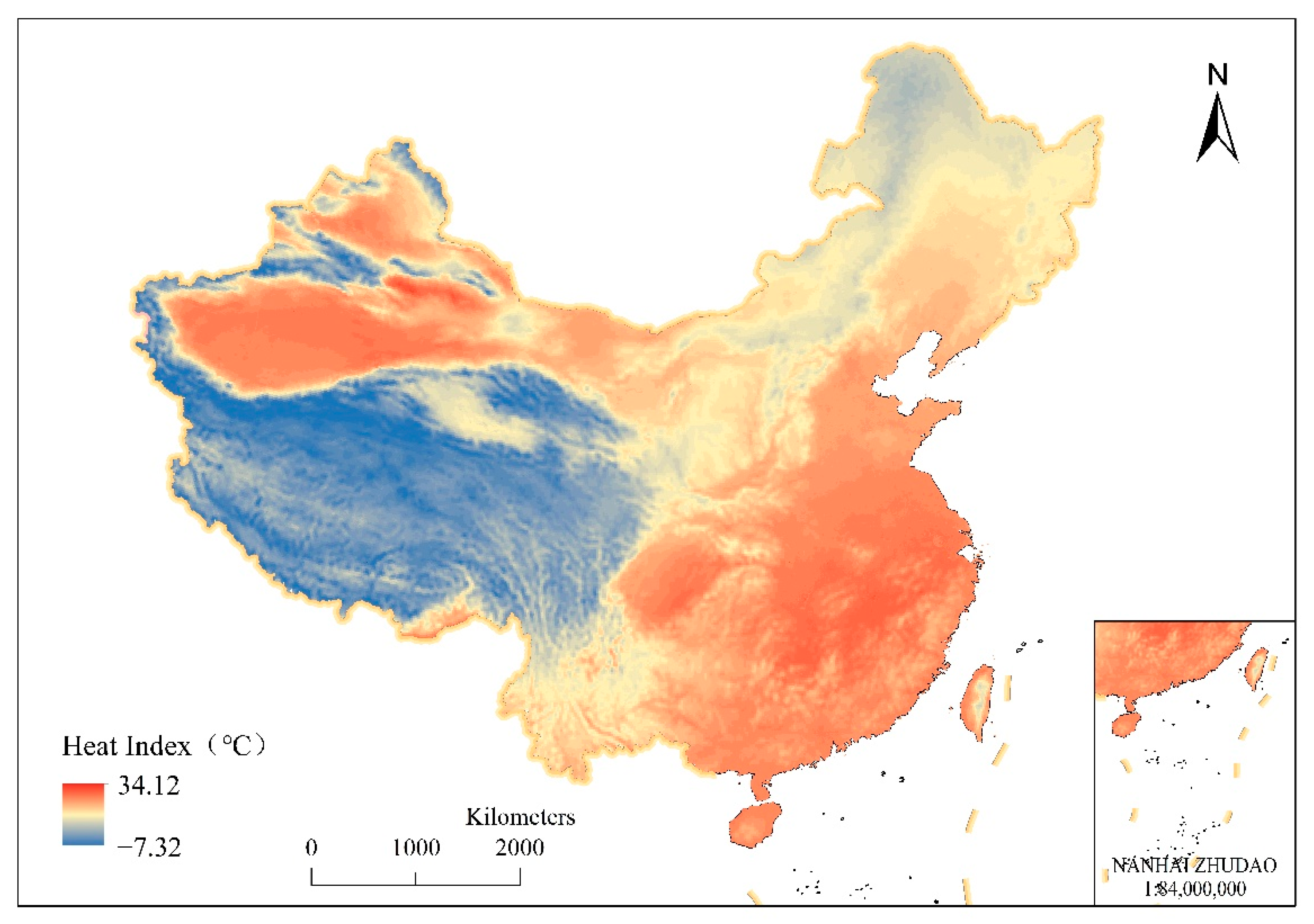
According to the HI calculation formula of the multiple linear regression model, the multi-source data we selected were substituted into the grid calculator tool using ArcMap v10.6 software. According to the calculation results, the mean daily HI in China during August 2020 was 20.51 °C; (ranged from −7.32 to 34.12 in the whole country); the distribution characteristics are shown in Figure 5.

3.3. Difference between HI and Air Temperature

To explore the difference between HI and air temperature spatial distribution, we subtracted the air temperature from HI. As shown in Figure 6, the HI in the northwest desert area was lower than the average temperature, while the HI values in the northeast and southern coastal areas were higher. The difference between the HI and average temperature in the central and western regions was within ±1.5 °C.

3.4. Calculation of the Number of Days with Heat Stress

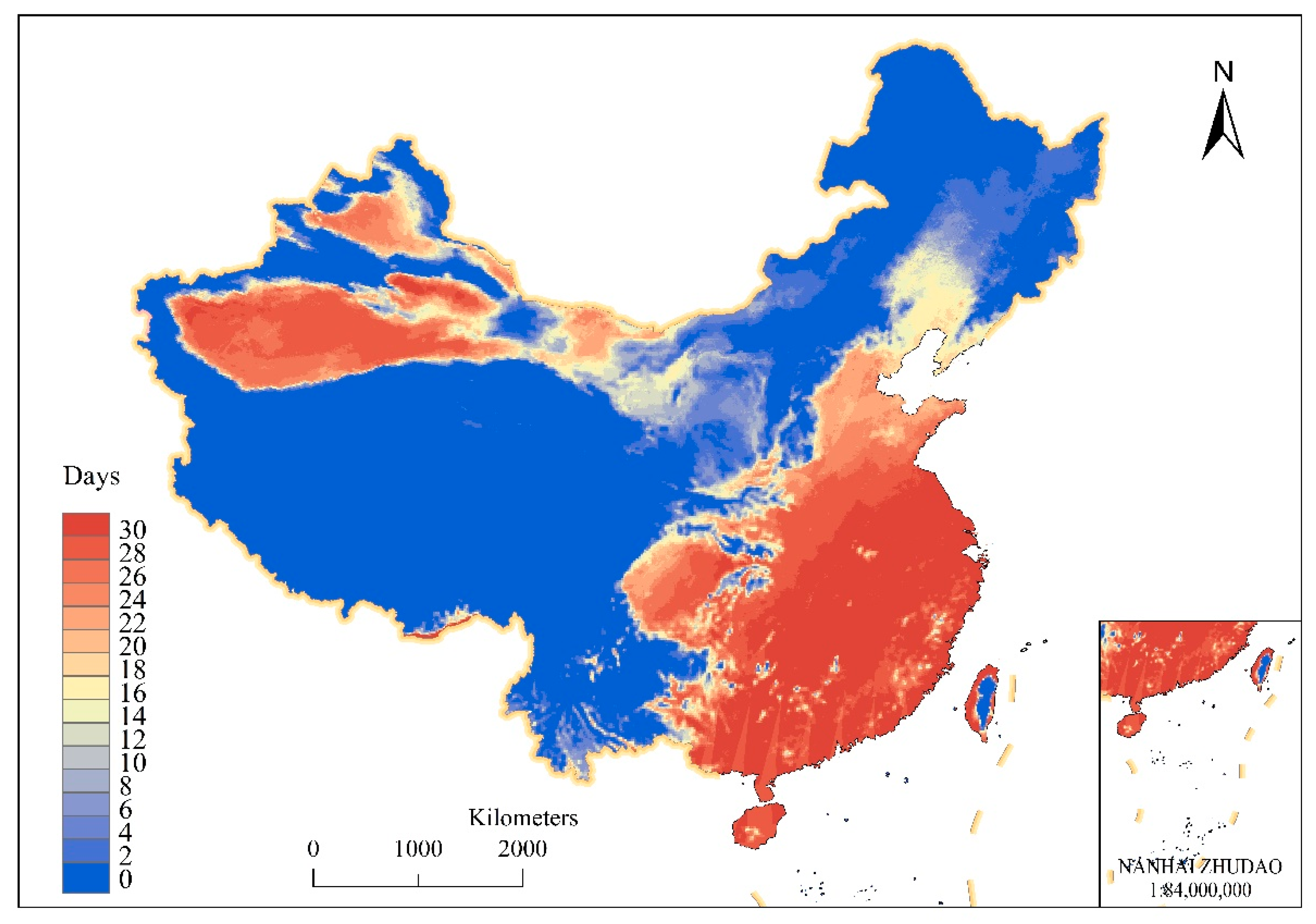
Equivalent temperature was divided according to the UTCI of thermal stress [55]. We calculated the number of days of the areas under heat stress with an HI > 26 °C (Figure 7). There were significant differences in the spatial distribution. The cumulative number of days of heat stress in coastal areas was much higher than in western plateau areas. Further area statistics showed that the areas with >20 days of heat stress in August accounted for 29.98% of the national area, 8.85% of the area with 10–20 days, and 61.17% of the area with <10 days. The southeast is densely populated, and the duration of thermal discomfort is long, factors that will seriously threaten the normal production and life activities of residents.

3.5. Variation in Daily Heat Stress Area Trends

According to the UTCI, we conducted area statistics on the areas with daily heat stress (Figure 8). We found that the area of heat stress area in early August was significantly higher than in late August, and the area changed significantly. In August, there were more than 13 days in which the heat stress area was >33% of the national area. Continuous large-scale heat discomfort will adversely affect residents, and it is urgently necessary to take effective measures to mitigate these conditions.

4. Discussion

4.1. Comparison with Previous Studies

The combination of multiple stepwise regression and multiple linear regression better reflected the effects of various factors on human comfort when calculating the daily HI. Compared to empirical models such as the humidex and HI and machine learning algorithms such as random forests, we found that the factors influencing comfort and their degree of influence changed over time, and that it is better to study human comfort through dynamically changing factors. Yin investigated the application of HI on human comfort [28]. Similarly, we used the meteorological station data to control and verify the accuracy of the HI during the HI calculation process. We improved the spatial continuity and resolution of the HI by adding multi-source data. The calculated daily MAE of 1 km HI was 1.49 °C, and the RMSE was 2.08 °C; thus, the accuracy was significantly improved, and the distribution characteristics of the HI were also consistent. Ren calculated the thermal comfort of 183 cities in China from 1990 to 2016 using daily meteorological station data [57]. Gobo also predicted future changes in climate comfort by kriging interpolation based on daily meteorological station data [58]. However, the spatial resolution of their results was relatively low. Ge used the ERA-Interim atmospheric reanalysis data to calculate the average UTCI from 1985 to 2014 on annual and seasonal scales to assess the thermal environment in China. The results revealed that the summer thermal heat stress area accounted for 20.25% of the total area in China, and this would be larger in July and August [56]. But the results of their study with low temporal and spatial resolution.

Our study area in China covered a wide range of latitudes and longitudes. The average HI of the meteorological stations was generally higher than the average regional HI. Therefore, the HI of the stations did not represent the overall effects of the region. To make up for this difference, we used a better universal division standard, the UTCI. Combined with the statistical calculation of daily heat stress area, our study on human comfort was more objective and intuitive. Previous studies showed that a relationship existed between human comfort and the number of deaths from various diseases [14,18,59,60]; therefore, it is beneficial to address extreme weather events through highly precise HI predictions.

Our study used daily scale data. Compared to long-term and small-scale HI studies [25], the effects of air temperature were dominant, and instantaneous changes in meteorological factors were prominent. In the final HI prediction model, we found that the resolution of air temperature was low, but its influence was high. Although other multi-source data had little influence, they could be used to improve the spatial continuity and resolution of the HI. Other multi-source data, although less influential, improved the spatial continuity and resolution of the HI. Generally, the results of the HI prediction model in this study were consistent with previous studies, but our prediction indicators were more comprehensive, and the prediction results were more accurate.

4.2. Improvements and Shortcomings

The main improvement of this study was that the HI obtained from the meteorological stations was used as the true HI value. Based on these values, multiple environmental variables were added to jointly invert the HI estimation. Thus, we had the advantage of a wide coverage area of multi-source data that effectively reduced the problem of the uneven spatial distribution of the meteorological stations and long distances between the stations. Through verification of the inversion results, the data had good fit. Additionally, the contribution of meteorological factors in our model was very high, indicating that meteorological factors greatly affect the HI. We also used the UTCI classification of human comfort to divide the average daily apparent temperature throughout the month. In addition, we calculated the change and regional distribution of the daily heat stress area.

However, our study did have some shortcomings. First, we selected only 376 national surface meteorological stations in China, and their elevations were relatively low, not representative of areas with higher elevations. Therefore, we were unable to account for the contribution of elevation in this study. Second, this study improved the spatial resolution of HI inversion by combining multi-source data, but the spatial resolution of the atmospheric reanalysis data was low (0.1°), a factor that inevitably affected the final inversion results. We need more accurate data added to the model for inversion and verification to improve the accuracy of HI inversion. In addition, we chose the multivariate stepwise regression model to screen the independent variables. We can try machine learning in future research to explore the optimal model for heat index calculation.

The results of this study will serve as a foundation for our future work. This experiment used nighttime light data to characterize the effects of urbanization expansion on the urban heat island effect, but the calculation results were not significant enough and its contribution was lower; thus, the selection of NTL for the characterization of urbanization expansion data requires further investigation. Additionally, the LST is an important influencing factor on temperature. In this experiment, owing to its high collinearity with TEMP, it was discarded. The collinearity between ATM and DEM was also high; therefore, we selected the DEM with higher product resolution as the inversion factor for the HI. The trade-off between the LST and mean TEMP, ATM, and DEM also requires further investigation.

5. Conclusions

China has a vast land area consisting of complex and diverse climates, significant differences in terrain, and large spatial differences in the HI. Based on the multi-source data extracted from the national meteorological stations, this study constructed a multiple regression equation for HI inversion through a multiple linear regression model and calculated the daily HI distribution characteristics in China during August 2020. Then, we used 10-fold cross-validation to estimate the model results. The value of R² was 0.95, the MAE was 1.80 °C, and the RMSE was 2.40 °C, showing a high degree of fit.

The daily daytime average values of the multi-source data were substituted in the multiple regression equation to obtain the mean daily HI distribution characteristics in China during August 2020. We also calculated the number of days with areas of heat stress; areas with >20 days of heat stress in August accounted for 29.98% of the national area, while 61.17% of the area had <10 days. The relatively high HI was mainly distributed in the desert areas in the northwest and the coastal areas in southeast China.

By combining atmospheric reanalysis data and multi-source data, this study accounted for the shortcomings of low spatial resolution of the atmospheric reanalysis data and discontinuous spatial distribution of the meteorological stations, thereby improving the accuracy of spatial distribution predictions of the HI. Collectively, these findings support the effects of the HI on human comfort.

References

1. Zhang, X.; Han, L.; Wei, H.; Tan, X.; Zhou, W.; Li, W.; Qian, Y. Linking urbanization and air quality together: A review and a perspective on the future sustainable urban development. J. Clean. Prod. 2022, 346, 130988. [Google Scholar] [CrossRef]
2. Zhan, Z.Y.; Zhong, X.; Yang, J.; Ding, Z.; Xie, X.X.; Zheng, Z.Q.; Hu, Z.J. Effect of apparent temperature on hospitalization from a spectrum of cardiovascular diseases in rural residents in Fujian, China. Environ. Pollut. 2022, 303, 119101. [Google Scholar] [CrossRef]
3. Giannopoulou, K.; Livada, I.; Santamouris, M.; Saliari, M.; Assimakopoulos, M.; Caouris, Y. The influence of air temperature and humidity on human thermal comfort over the greater Athens area. Sustain. Cities Soc. 2014, 10, 184–194. [Google Scholar] [CrossRef]
4. Song, C.; Duan, G.; Wang, D.; Liu, Y.; Du, H.; Chen, G. Study on the influence of air velocity on human thermal comfort under non-uniform thermal environment. Build. Environ. 2021, 196, 107808. [Google Scholar] [CrossRef]
5. Yin, J.; Tan, J.G.; Zhu, L.M.; Wang, J.Y.; Zhao, Y. Correlation Analysis between Chronic Obstructive Pulmonary Disease and Meteorological Factors in Different Areas. 2007, 35, 841–844.
6. Yue, H.Y.; Shen, S.H. Advance in the relationship between respiratory and cardio-cerebrovascular diseases and meteorological conditions. J. Meteorol. Environ. 2009, 25, 57–61. [Google Scholar] [CrossRef]
7. Ho, H.C.; Knudby, A.; Xu, Y.; Hodul, M.; Aminipouri, M. A comparison of urban heat islands mapped using skin temperature, air temperature, and apparent temperature (Humidex), for the greater Vancouver area. Sci. Total Environ. 2016, 544, 929–938. [Google Scholar] [CrossRef] [PubMed]
8. Steadman, R.G. Indices of Windchill of Clothed Persons. J. Appl. Meteorol. Climatol. 1971, 10, 674–683. [Google Scholar] [CrossRef]
9. Steadman, R.G. The Assessment of Sultriness. Part I: A Temperature-Humidity Index Based on Human Physiology and Clothing Science. J. Appl. Meteorol. Climatol. 1979, 18, 861–873. [Google Scholar] [CrossRef]
10. Wichmann, J. Heat effects of ambient apparent temperature on all-cause mortality in Cape Town, Durban and Johannesburg, South Africa: 2006–2010. Sci. Total Environ. 2017, 587–588, 266–272. [Google Scholar] [CrossRef] [PubMed] [Green Version]
11. Oppermann, E.; Kjellstrom, T.; Lemke, B.; Otto, M.; Lee, J.K.W. Establishing intensifying chronic exposure to extreme heat as a slow onset event with implications for health, wellbeing, productivity, society and economy. Curr. Opin. Environ. Sustain. 2021, 50, 225–235. [Google Scholar] [CrossRef]
12. Bisanti, L.; Cadum, E.; Costa, G.; Michelozzi, P.; Perucci, C.; Russo, A.J.E. 2003 Heat Waves and Mortality in Italy. Epidemiology 2004, 15, S97. [Google Scholar] [CrossRef]
13. Nagano, K.; Horikoshi, T. Development of outdoor thermal index indicating universal and separate effects on human thermal comfort. Int. J. Biometeorol. 2011, 55, 219–227. [Google Scholar] [CrossRef]
14. Keatinge, W.R.; Donaldson, G.C.; Cordioli, E.; Martinelli, M.; Kunst, A.E.; Mackenbach, J.P.; Nayha, S.; Vuori, I. Heat related mortality in warm and cold regions of Europe: Observational study. BMJ 2000, 321, 670–673. [Google Scholar] [CrossRef] [PubMed] [Green Version]
15. Vanos, J.K.; Warland, J.S.; Gillespie, T.J.; Kenny, N.A. Review of the physiology of human thermal comfort while exercising in urban landscapes and implications for bioclimatic design. Int. J. Biometeorol. 2010, 54, 319–334. [Google Scholar] [CrossRef]
16. Fanger, P. Thermal Comfort: Analysis and Applications in Environmental Engineering; Danish Technical Press: Copenhagen, Denmark, 1972. [Google Scholar]
17. Yan, Y.; Yue, S.; Hui, C.; Liu, X.; Yan, Y.C.; Yue, S.P.; Liu, X.H.; Wang, D.D.; Chen, H. Advances on Assessment of Bioclimatic Comfort Conditions at Home and Abroad. Adv. Earth Sci. 2013, 28, 1119–1125. [Google Scholar]
18. Li, J.Y.; Ma, X.P.; Wang, S.G.; Ying, Z.; Shang, K.Z. Analysis of the relationship between diseases of the circulatoryrespiratory system and felt air temperature in Nanjing City with the GAM model. J. Lanzhou Univ. (Nat. Sci.) 2015, 51, 659–664. [Google Scholar] [CrossRef]
19. Guisan, A.; Edwards, T.C., Jr.; Hastie, T. Generalized linear and generalized additive models in studies of species distributions: Setting the scene. J. Ecol. Model. 2002, 157, 89–100. [Google Scholar] [CrossRef] [Green Version]
20. Ma, P.; Wang, S.G.; Shang, K.Z.; Li, T.S.; Yin, L.J. The impact of meteorological comfort conditions on respiratory disease. China Environ. Sci. 2018, 38, 374–382. [Google Scholar]
21. Yang, J.J. The comprehensive evaluation of suitability of summer tourism base in China. Res. Sci. 2016, 38, 11–16. [Google Scholar]
22. QX/T 500-2019; Evaluation Method of Climate Suitability for the Cool Summer Tourism. Chinese Industry Standard: Beijing China, 2019.
23. Mei, L.; Bo, Y.; Yao, K. The apparent temperature model based on thermal equilibrium and effect of climatic elements. J. Nanjing Institut. Meteorol. 2001, 4, 527–535. [Google Scholar] [CrossRef]
24. Zhu, S.Y.; Gao, T.; Wang, L.; Yang, D.; Zeng, Y.Q. Study on calculation method of somatosensory temperature. J. Technol. Innov. Appl. 2020, 22, 116–117. [Google Scholar]
25. Steadman, R.G. A Universal Scale of Apparent Temperature. J. Appl. Meteorol. Climatol. 1984, 23, 1674–1687. [Google Scholar] [CrossRef]
26. Masterton, J.M.; Richardson, F.A. Humidex: A Method of Quantifying Human Discomfort Due to Excessive Heat and Humidity; Environment Canada, Atmospheric Environment: Gatineau, QC, Canada, 1979. [Google Scholar]
27. Li, N.; Xu, Y.M.; He, M.; Wu, X.H. Retrieval of Apparent Temperature in Beijing Based on Remote Sensing. Ecol. Environ. Sci. 2018, 27, 1113–1121. [Google Scholar]
28. Yin, C.; Yang, F.; Wang, J.; Ye, Y. Spatiotemporal Distribution and Risk Assessment of Heat Waves Based on Apparent Temperature in the One Belt and One Road Region. Remote Sens. 2020, 12, 1174. [Google Scholar] [CrossRef] [Green Version]
29. Höppe, P. The physiological equivalent temperature—A universal index for the biometeorological assessment of the thermal environment. Int. J. Biometeorol. 1999, 43, 71–75. [Google Scholar] [CrossRef]
30. Jendritzky, G.; De, D.R.; Havenith, G. UTCI—Why another thermal index? Int. J. Biometeorol. 2012, 56, 421–428. [Google Scholar] [CrossRef] [Green Version]
31. Gagge, A.P.; Stolwijk, J.A.J.; Nishi, Y. An Effective Temperature Scale Based on a Simple Model of Human Physiological Regulatory Response; Memoirs of the Faculty of Engineering, Hokkaido University: Sapporo, Japan, 1971; Volume 77, pp. 21–36. [Google Scholar]
32. Höppe, P. Die Energiebilanz des Menschen (Dissertation). Wiss. Mitt. Met. Inst. 1984; 49. [Google Scholar]
33. Rothfusz, L. The Heat Index Equation; National Oceanic and Atmospheric Administration, National Weather Service, Office of Meteorology: Fort Worth, TX, USA, 1990. [Google Scholar]
34. Feng, L.; Zhao, M.; Zhou, Y.; Zhu, L.; Tian, H. The seasonal and annual impacts of landscape patterns on the urban thermal comfort using Landsat. Ecol. Indic. 2020, 110, 105798. [Google Scholar] [CrossRef]
35. Zhu, X.; Hou, C.; Xu, K.; Liu, Y. Establishment of agricultural drought loss models: A comparison of statistical methods. Ecol. Indic. 2020, 112, 106084. [Google Scholar] [CrossRef]
36. Aretouyap, Z.; Domra Kana, J.; Kemgang Ghomsi, F.E. Appraisal of environment quality in the capital district of Cameroon using Landsat-8 images. Sustain. Cities Soc. 2021, 67, 102734. [Google Scholar] [CrossRef]
37. Sharma, R.; Pradhan, L.; Kumari, M.; Bhattacharya, P. Assessing urban heat islands and thermal comfort in Noida City using geospatial technology. Urban Clim. 2021, 35, 100751. [Google Scholar] [CrossRef]
38. Mandal, J.; Patel, P.P.; Samanta, S. Examining the expansion of Urban Heat Island effect in the Kolkata Metropolitan Area and its vicinity using multi-temporal MODIS satellite data. Adv. Space Res. 2022, 69, 1960–1977. [Google Scholar] [CrossRef]
39. Du, H.; Cai, W.; Xu, Y.; Wang, Z.; Wang, Y.; Cai, Y. Quantifying the cool island effects of urban green spaces using remote sensing Data. Urban For. Urban Green. 2017, 27, 24–31. [Google Scholar] [CrossRef]
40. Xu, J.; Wei, Q.; Huang, X.; Zhu, X.; Li, G. Evaluation of human thermal comfort near urban waterbody during summer. Build. Environ. 2010, 45, 1072–1080. [Google Scholar] [CrossRef]
41. Vandentorren, S.; Bretin, P.; Zeghnoun, A.; Mandereau-Bruno, L.; Croisier, A.; Cochet, C.; Ribéron, J.; Siberan, I.; Declercq, B.; Ledrans, M. August 2003 Heat Wave in France: Risk Factors for Death of Elderly People Living at Home. Eur. J. Public Health 2006, 16, 583–591. [Google Scholar] [CrossRef] [Green Version]
42. Mansour, K.; Aziz, M.A.; Hashim, S.; Effat, H. Impact of anthropogenic activities on urban heat islands in major cities of El-Minya Governorate, Egypt. Egypt. J. Remote Sens. Space Sci. 2022, 25, 609–620. [Google Scholar] [CrossRef]
43. Hersbach, H.; Bell, B.; Berrisford, P.; Horányi, A.; Sabater, J.M.; Nicolas, J.; Radu, R.; Schepers, D.; Simmons, A.; Soci, C.; et al. Global Reanalysis: Goodbye ERA-Interim, Hello ERA5. In ECMWF Newsletter No. 159; Lentze, G., Ed.; European Centre for Medium-Range Weather Forecasts (ECMWF): Reading, UK, 2019; pp. 17–24. [Google Scholar]
44. Román, M.O.; Wang, Z.; Sun, Q.; Kalb, V.; Miller, S.D.; Molthan, A.; Schultz, L.; Bell, J.; Stokes, E.C.; Pandey, B.; et al. NASA’s Black Marble nighttime lights product suite. Remote Sens. Environ. 2018, 210, 113–143. [Google Scholar] [CrossRef]
45. McCutchan, M.H.; Fox, D.G. Effect of Elevation and Aspect on Wind, Temperature and Humidity. J. Clim. Appl. Meteorol. 1986, 25, 1996–2013. [Google Scholar] [CrossRef]
46. Muthusamy, M.; Casado, M.R.; Butler, D.; Leinster, P. Understanding the effects of Digital Elevation Model resolution in urban fluvial flood modelling. J. Hydrol. 2021, 596, 126088. [Google Scholar] [CrossRef]
47. Gressner, A.M.; Arndt, T. Lexikon der Medizinischen Laboratoriumsdiagnostik; Springer: Berlin/Heidelberg, Germany, 2013. [Google Scholar]
48. Li, J.; Chen, Y.D.; Gan, T.Y.; Lau, N.-C. Elevated increases in human-perceived temperature under climate warming. Nat. Clim. Chang. 2018, 8, 43–47. [Google Scholar] [CrossRef]
49. Lawrence, M.G. The Relationship between Relative Humidity and the Dewpoint Temperature in Moist Air: A Simple Conversion and Applications. Bull. Am. Meteorol. Soc. 2005, 86, 225–234. [Google Scholar] [CrossRef]
50. Li, Y.; Fan, T.; Zhao, C.; Yang, X.; Zhou, P.; Li, K. Quantifying the Long-Term MODIS Cloud Regime Dependent Relationship between Aerosol Optical Depth and Cloud Properties over China. Remote Sens. 2022, 14, 3844. [Google Scholar] [CrossRef]
51. James, G.; Witten, D.; Hastie, T.; Tibshirani, R. Resampling Methods. In An Introduction to Statistical Learning: With Applications in R; James, G., Witten, D., Hastie, T., Tibshirani, R., Eds.; Springer: New York, NY, USA, 2013; pp. 175–201. [Google Scholar]
52. Saud, S.; Jamil, B.; Upadhyay, Y.; Irshad, K. Performance improvement of empirical models for estimation of global solar radiation in India: A k-fold cross-validation approach. Sustain. Energy Technol. Assess. 2020, 40, 100768. [Google Scholar] [CrossRef]
53. Burnham, K.P.; Anderson, D.R. Multimodel Inference: Understanding AIC and BIC in Model Selection. Sociol. Methods Res. 2004, 33, 261–304. [Google Scholar] [CrossRef]
54. O’brien, R.M. A Caution Regarding Rules of Thumb for Variance Inflation Factors. Qual. Quant. 2007, 41, 673–690. [Google Scholar] [CrossRef]
55. Bröde, P.; Fiala, D.; Błażejczyk, K.; Holmér, I.; Jendritzky, G.; Kampmann, B.; Tinz, B.; Havenith, G. Deriving the operational procedure for the Universal Thermal Climate Index (UTCI). Int. J. Biometeorol. 2012, 56, 481–494. [Google Scholar] [CrossRef] [PubMed]
56. Ge, Q.; Kong, Q.; Xi, J.; Zheng, J. Application of UTCI in China from tourism perspective. Theor. Appl. Climatol. 2016, 128, 551–561. [Google Scholar] [CrossRef]
57. Ren, Z.; Fu, Y.; Dong, Y.; Zhang, P.; He, X. Rapid urbanization and climate change significantly contribute to worsening urban human thermal comfort: A national 183-city, 26-year study in China. Urban Clim. 2022, 43, 101154. [Google Scholar] [CrossRef]
58. Gobo, J.P.A.; Wollmann, C.A.; Celuppi, M.C.; Galvani, E.; Faria, M.R.; Mendes, D.; de Oliveira-Júnior, J.F.; dos Santos Malheiros, T.; Riffel, E.S.; Gonçalves, F.L.T. The bioclimate present and future in the state of são paulo/brazil: Space-time analysis of human thermal comfort. Sustain. Cities Soc. 2022, 78, 103611. [Google Scholar] [CrossRef]
59. Hajat, S.; Kovats, R.S.; Atkinson, R.W.; Haines, A. Impact of hot temperatures on death in London: A time series approach. J. Epidemiol. Community Health 2002, 56, 367–372. [Google Scholar] [CrossRef] [PubMed] [Green Version]
60. Fouillet, A.; Rey, G.; Laurent, F.; Pavillon, G.; Bellec, S.; Guihenneuc-Jouyaux, C.; Clavel, J.; Jougla, E.; Hémon, D. Excess mortality related to the August 2003 heat wave in France. Int. Arch. Occup. Environ. Health 2006, 80, 16–24. [Google Scholar] [CrossRef]
Figure 1. Distribution of the surface meteorological stations in China on the ASTER Global Digital Elevation Map (GDEM).
Remotesensing 14 04999 g001
Figure 2. Correlation of (a) average temperature and (b) dewpoint temperature between the meteorological station data and ERA-5 atmospheric reanalysis data.
Remotesensing 14 04999 g002
Figure 3. The technical method for calculating the distribution of thermal comfort areas and cumulative heat stress duration days in this study.
Remotesensing 14 04999 g003
Figure 4. Correlation analysis between the estimated and meteorological station HI values.
Remotesensing 14 04999 g004
Figure 5. The mean HIs in China during August 2020.
Remotesensing 14 04999 g005
Figure 6. Difference between the HI and air temperature.
Remotesensing 14 04999 g006
Figure 7. The duration of heat stress in China in August 2020.
Remotesensing 14 04999 g007
Figure 8. Area statistics of daily heat stress area. The red columns indicate that the area of heat stress exceeds 33% of the country’s land area, while the blue columns indicate that it does not.
Remotesensing 14 04999 g008