
Comparison of Land Use Land Cover Classifiers Using Different Satellite Imagery and Machine Learning Techniques


 ,
,  , and
, and
Abstract
1. Introduction
2. Data and Methods
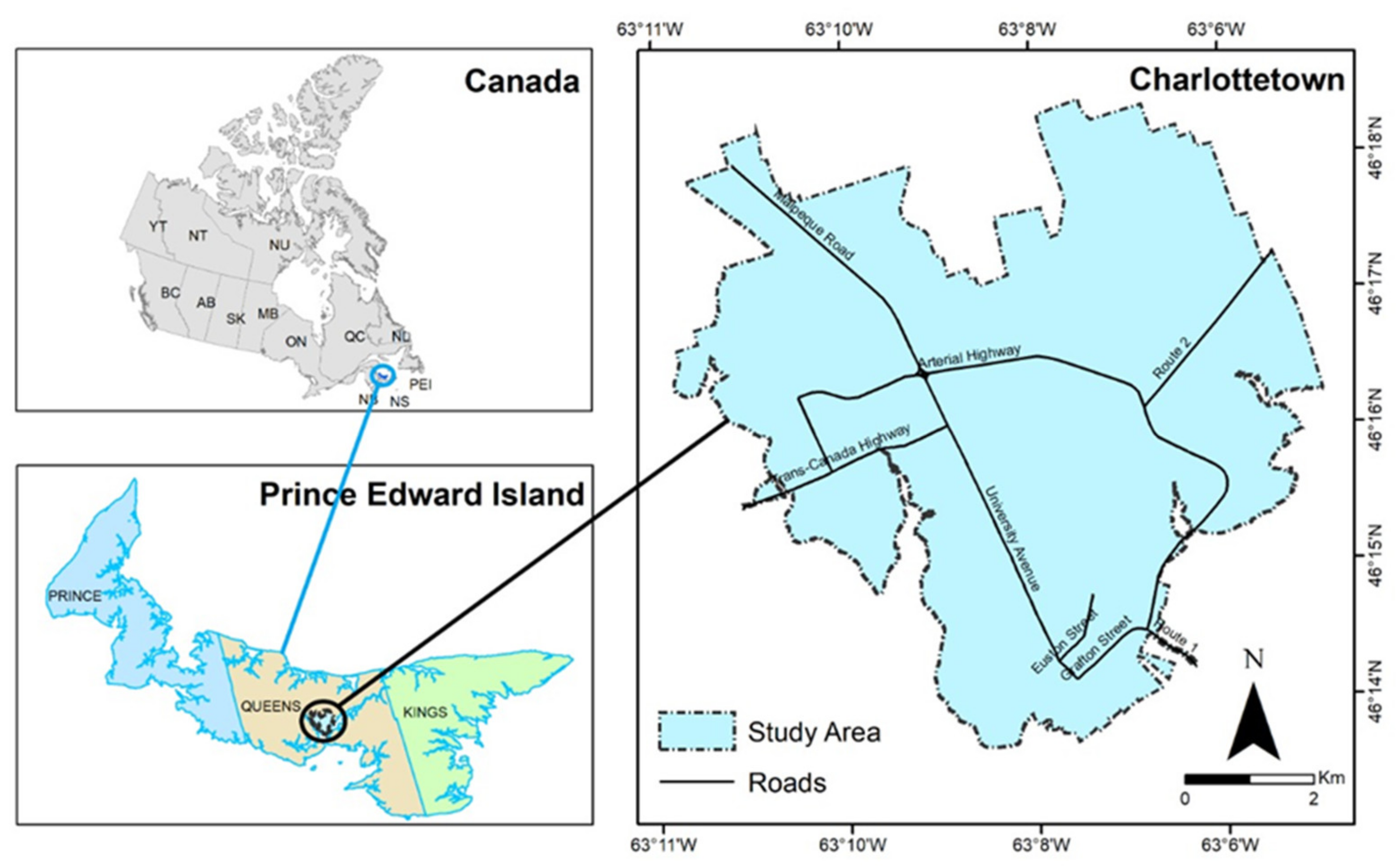
2.1. Study Area
2.2. Satellite Data
- Landsat 8: the Landsat program is a component of the USGS National Land Imaging (NLI) Program, which has ensured continuity, reliability, and comparability of data since 1974. Landsat has a spatial resolution of 30 m [43].
- Sentinel 2: Sentinel 2 is a high-resolution (10 m), wide-swath, and multispectral imaging system. This aids Copernicus land monitoring studies, such as the examination of water cover and water bodies, vegetation, soil, and the observation related to coastal areas and inland water cover. Sentinel 2 contains thirteen spectral bands [44].
- Planet: since 2016, Planet has captured multispectral photography for consumer use. Planet imagery has high-resolution (3–5 m) imagery that is becoming an essential resource for earth imaging [45]. Planet Scope has more than 150 nanosatellites with a unique combination (coverage of the area, frequency, and high resolution) that can take daily images at a 3 m resolution [25]. These datasets are much more helpful for a better understanding of LULC changes.
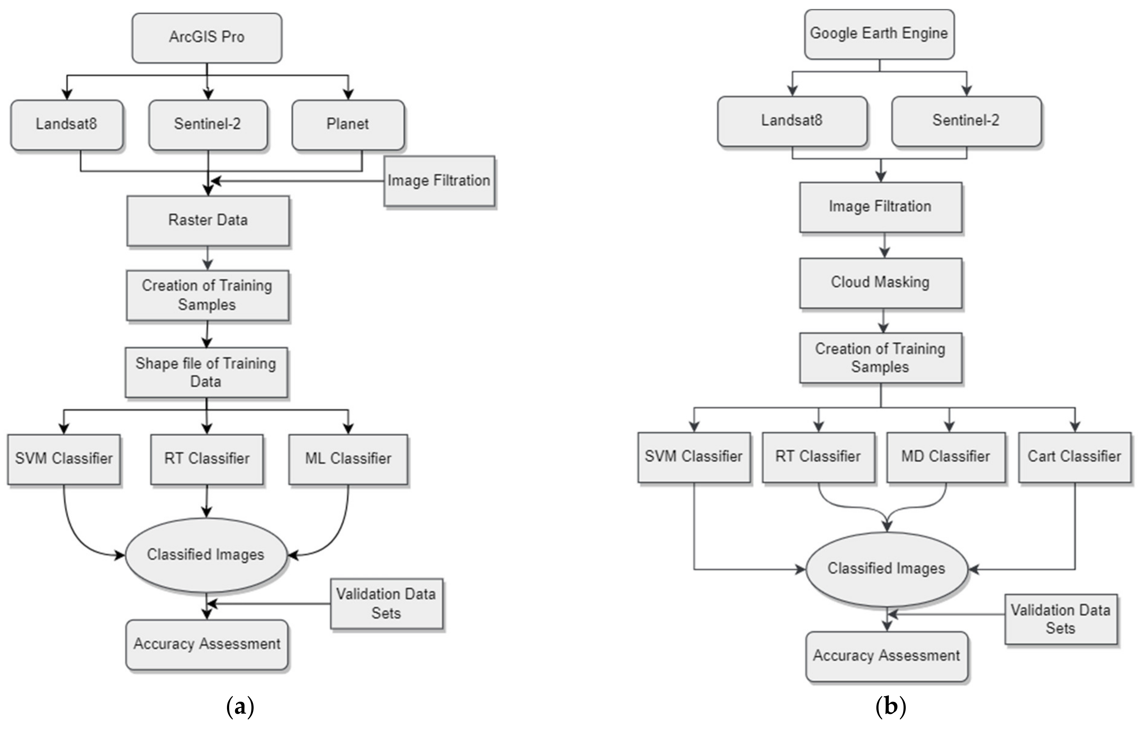
2.3. Methodological Framework for LULC Classification
2.4. Classification Methods
- Classification and regression tree (CART) is a decision classification tree that facilitates straightforward decision-making and regression analyses [47]. Based on a predetermined threshold, CART runs by separating nodes until it reaches the terminal nodes. This method divides input data into further group sets, and trees are generated using all but one of those group sets. The “classifier.smileCart” approach, which is part of the Google Earth Engine library, was used in this project.
- Random forest/random tree (RF/RT) RF/RT constructs an ensemble classifier and is one of the commonly used classifiers [48] by mixing many CART. RF/RT generates many decision trees using a random selection of training datasets and factors. The two most essential input criteria for this classifier are the size of the training dataset, and the number of trees generated [49,50].
- Support vector machine (SVM). One of the supervised learning techniques is SVM which is used to resolve different problems related to regression and classifications. In the training phase, SVM classifiers generate an ideal hyperplane that splits several classes with the less misclassified pixels from input datasets. The kernel functions, cost parameters, and gamma [51] are key parameters for determining support vectors.
- Minimum distance classifier (MD). The MD classifier classifies imagery datasets into classes that reduce the distance between the class in multi-feature space and image data. This distance between the image data is expressed as a similarity index, such that the minimal distance and highest similarity are equivalent. The main idea behind this process is to calculate the spectral distance between the measurement vector for the candidate pixel and the mean vector for each signature [52].
- Maximum likelihood classifier (ML). Maximum likelihood classifier is a supervised classification method that describes every band by a normal distribution. This supervised classification method is based on the Byes theorem [53].
2.5. Data Processing
2.6. Accuracy Assessment
2.7. Change Detection
3. Results and Discussion
3.1. LULC Classification Maps
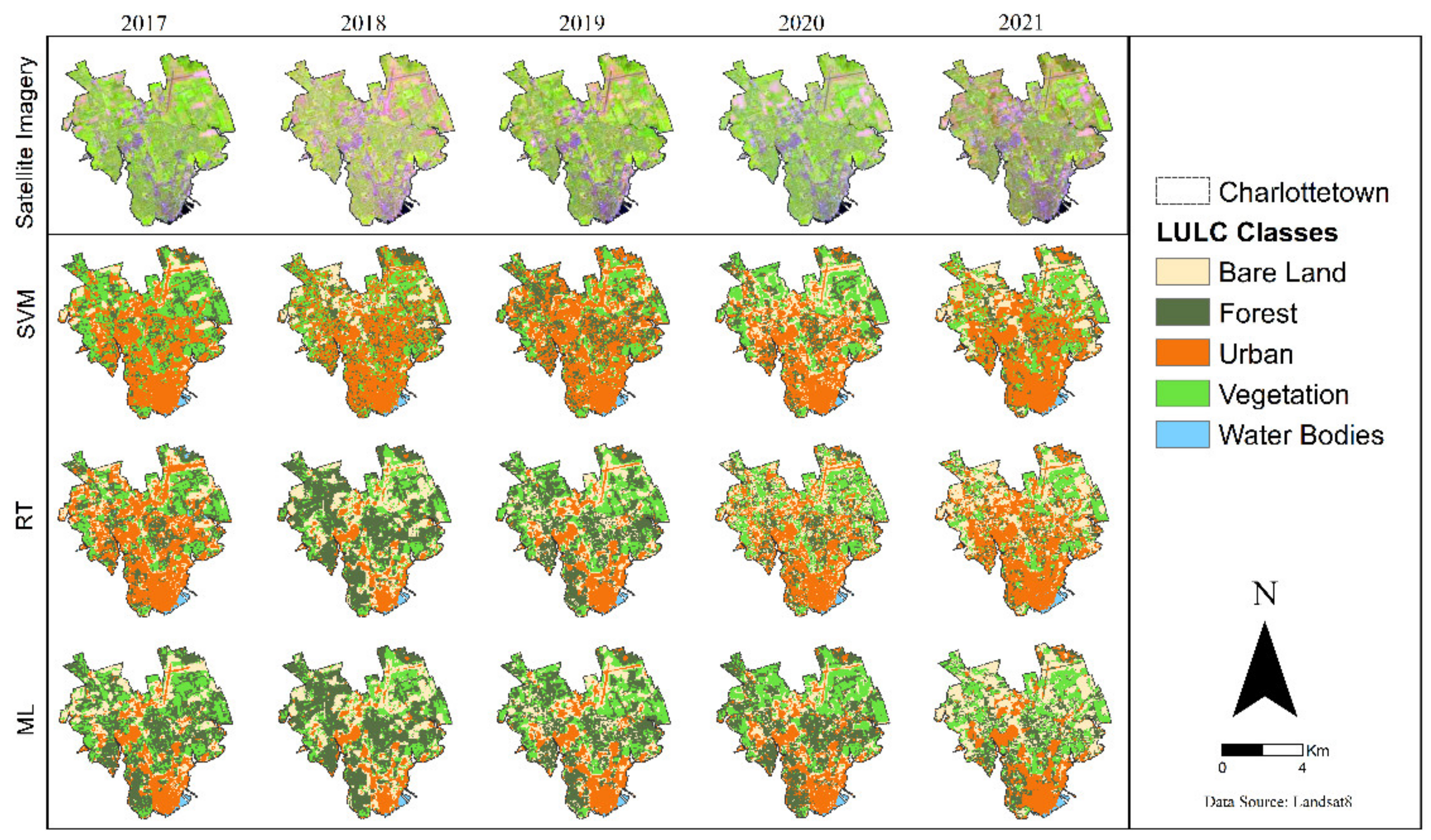
3.1.1. LULC Classification of Landsat 8 Imagery in ArcGIS Pro
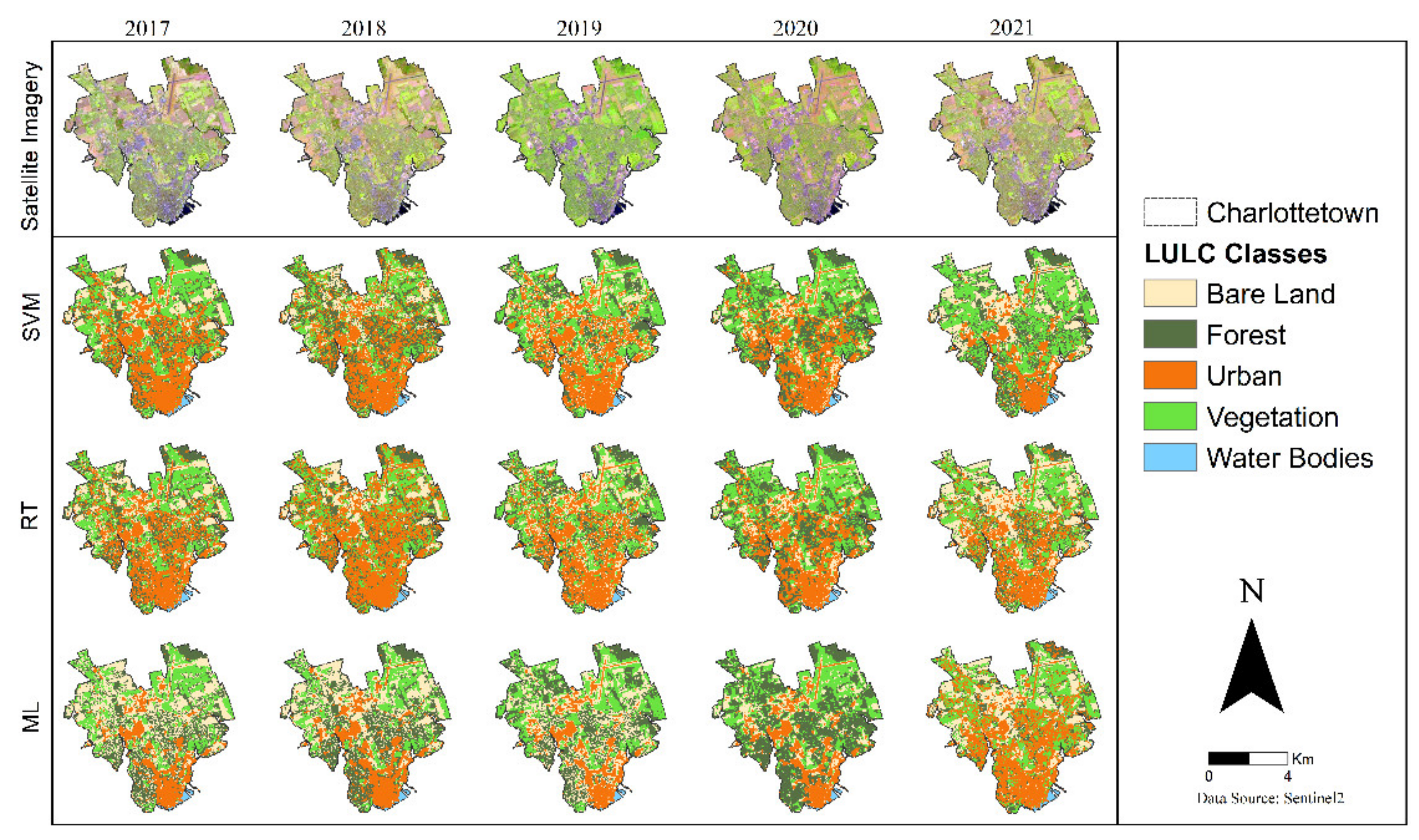
3.1.2. LULC Classification of Sentinel 2 Imagery in ArcGIS Pro
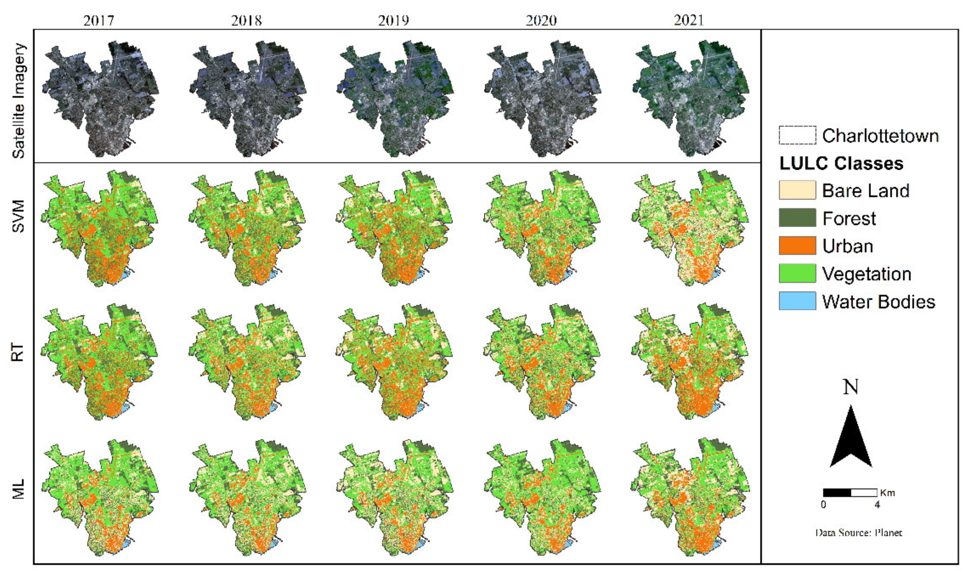
3.1.3. LULC Classification of Planet Imagery in ArcGIS Pro
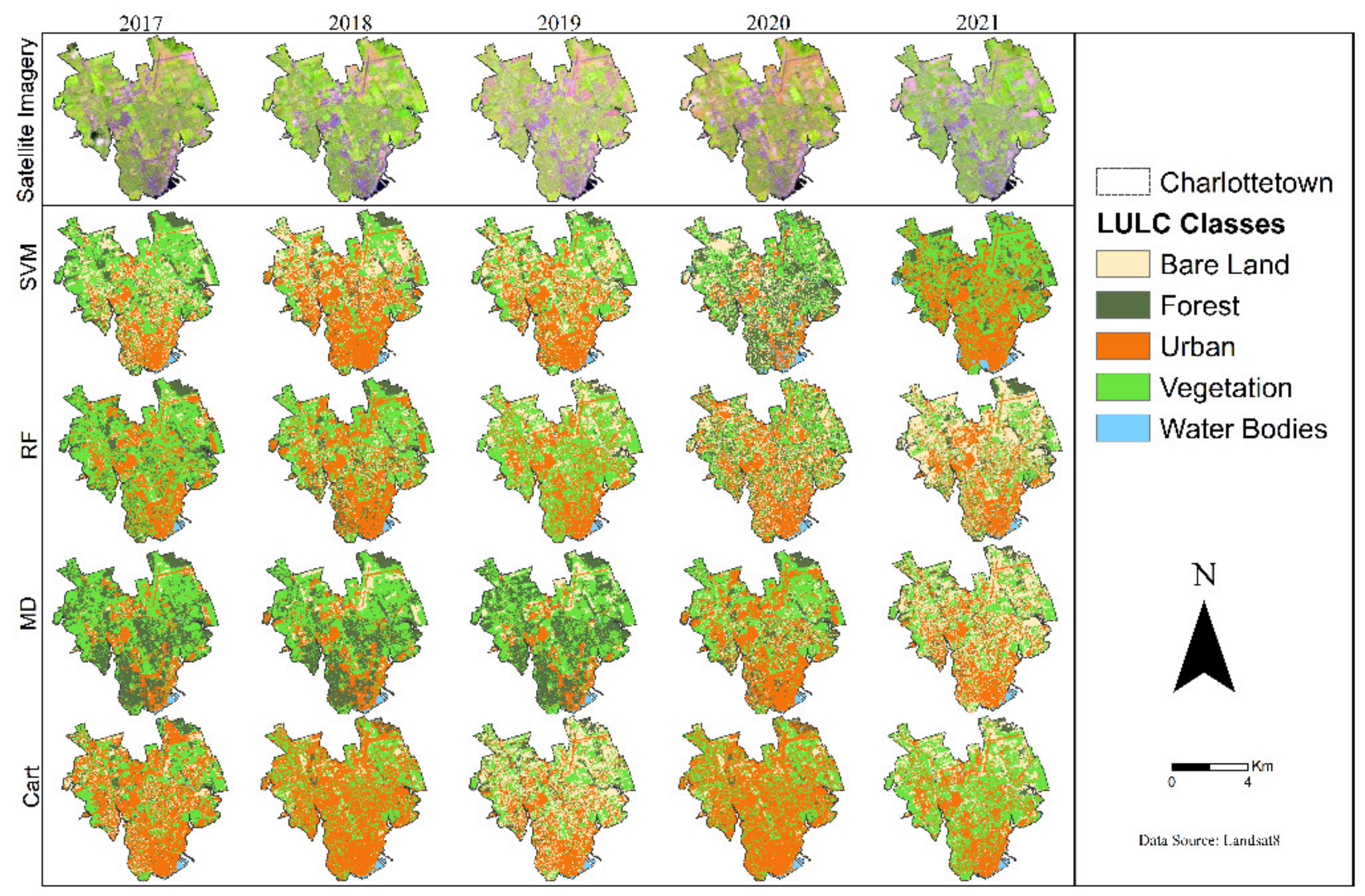
3.1.4. LULC Classification of Landsat 8 Imagery in Google Earth Engine
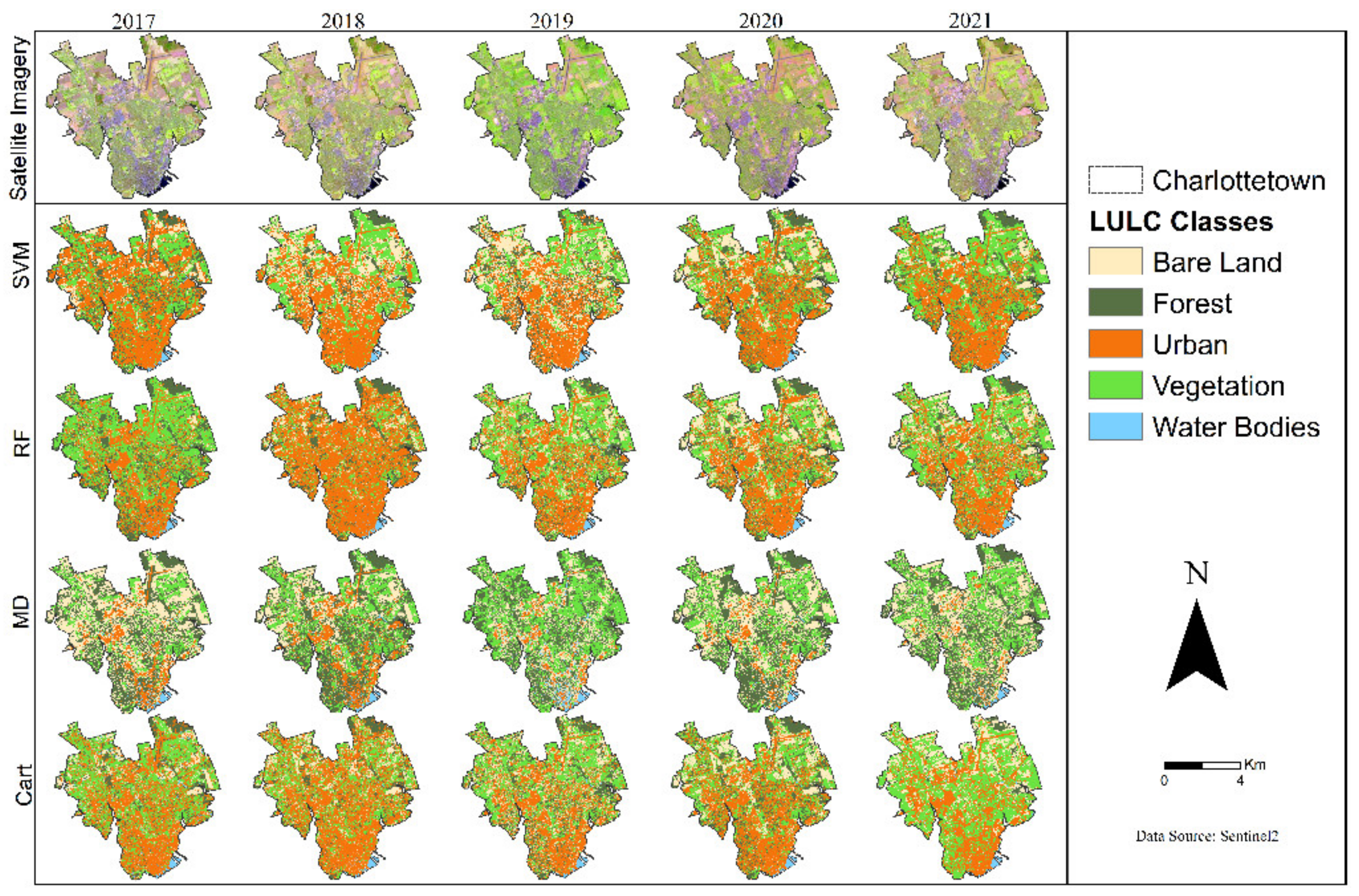
3.1.5. LULC Classification of Sentinel 2 Imagery in Google Earth Engine
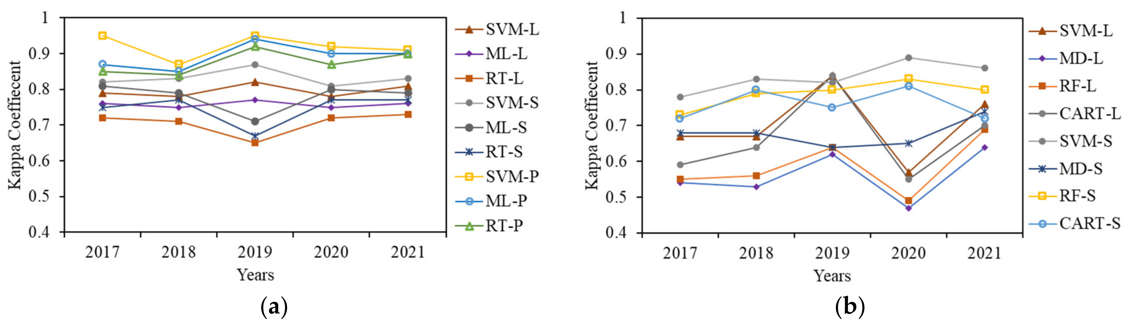
3.2. Accuracy Assessment
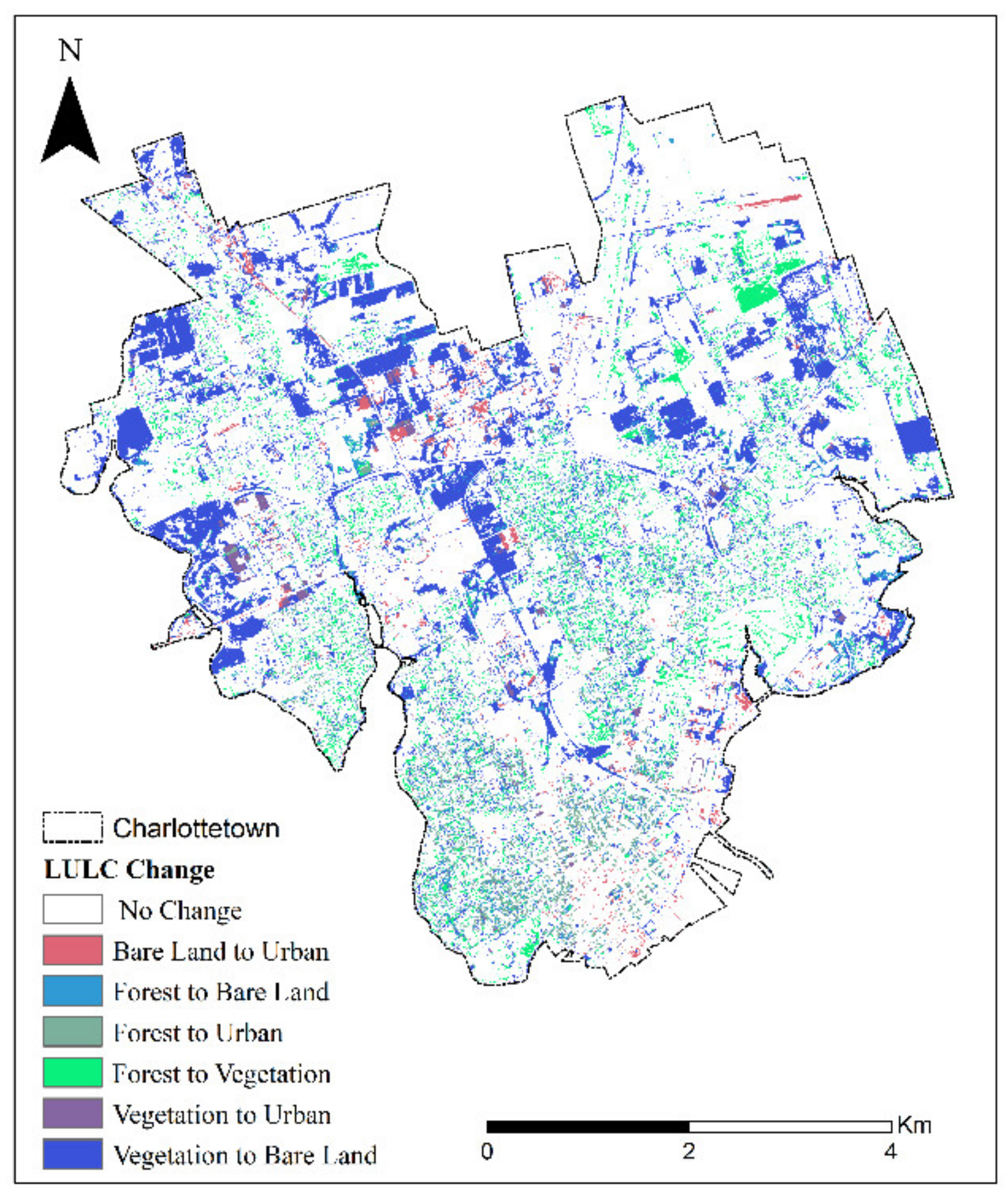
3.3. Change Detection
4. Conclusions
Author Contributions
Funding
Data Availability Statement
Conflicts of Interest
References
- Li, Y.; Brando, P.M.; Morton, D.C.; Lawrence, D.M.; Yang, H.; Randerson, J.T. Deforestation-induced climate change reduces carbon storage in remaining tropical forests. Nat. Commun. 2022, 13, 1964. [Google Scholar] [CrossRef] [PubMed]
- Sridhar, V.; Kang, H.; Ali, S.A. Human-Induced Alterations to Land Use and Climate and Their Responses for Hydrology and Water Management in the Mekong River Basin. Water 2019, 11, 1307. [Google Scholar] [CrossRef]
- Sridhar, V.; Jin, X.; Jaksa, W.T.A. Explaining the hydroclimatic variability and change in the Salmon River basin. Clim. Dyn. 2012, 40, 1921–1937. [Google Scholar] [CrossRef]
- Sujatha, E.; Sridhar, V. Spatial Prediction of Erosion Risk of a Small Mountainous Watershed Using RUSLE: A Case-Study of the Palar Sub-Watershed in Kodaikanal, South India. Water 2018, 10, 1608. [Google Scholar] [CrossRef]
- Sridhar, V.; Billah, M.M.; Hildreth, J.W. Coupled Surface and Groundwater Hydrological Modeling in a Changing Climate. Groundwater 2017, 56, 618–635. [Google Scholar] [CrossRef] [PubMed]
- Xiao, Y.; Liu, K.; Yan, H.; Zhou, B.; Huang, X.; Hao, Q.; Zhang, Y.; Zhang, Y.; Liao, X.; Yin, S. Hydrogeochemical constraints on groundwater resource sustainable development in the arid Golmud alluvial fan plain on Tibetan plateau. Environ. Earth Sci. 2021, 80, 750. [Google Scholar] [CrossRef]
- Xiao, Y.; Xiao, D.; Hao, Q.; Liu, K.; Wang, R.; Huang, X.; Liao, X.; Zhang, Y. Accessible Phreatic Groundwater Resources in the Central Shijiazhuang of North China Plain: Perspective From the Hydrogeochemical Constraints. Front. Environ. Sci. 2021, 9, 475. [Google Scholar] [CrossRef]
- Xiao, Y.; Hao, Q.; Zhang, Y.; Zhu, Y.; Yin, S.; Qin, L.; Li, X. Investigating Sources, Driving Forces and Potential Health Risks of Nitrate and Fluoride in Groundwater of a Typical Alluvial Fan Plain. Sci. Total Environ. 2022, 802, 149909. [Google Scholar] [CrossRef]
- Sridhar, V.; Ali, S.A.; Sample, D.J. Systems Analysis of Coupled Natural and Human Processes in the Mekong River Basin. Hydrology 2021, 8, 140. [Google Scholar] [CrossRef]
- Jamali, B.; Bach, P.M.; Cunningham, L.; Deletic, A. A Cellular Automata Fast Flood Evaluation (CA-ffé) Model. Water Resour. Res. 2019, 55, 4936–4953. [Google Scholar] [CrossRef]
- Rahman, A.; Abdullah, H.M.; Tanzir, M.T.; Hossain, M.J.; Khan, B.M.; Miah, M.G.; Islam, I. Performance of Different Machine Learning Algorithms on Satellite Image Classification in Rural and Urban Setup. Remote Sens. Appl. Soc. Environ. 2020, 20, 100410. [Google Scholar] [CrossRef]
- Sridhar, V.; Anderson, K.A. Human-Induced Modifications to Land Surface Fluxes and Their Implications on Water Management under Past and Future Climate Change Conditions. Agric. For. Meteorol. 2017, 234–235, 66–79. [Google Scholar] [CrossRef]
- Cihlar, J. Land Cover Mapping of Large Areas from Satellites: Status and Research Priorities. Int. J. Remote Sens. 2000, 21, 1093–1114. [Google Scholar] [CrossRef]
- Renschler, C.S.; Harbor, J. Soil Erosion Assessment Tools from Point to Regional Scales—The Role of Geomorphologists in Land Management Research and Implementation. Geomorphology 2002, 47, 189–209. [Google Scholar] [CrossRef]
- Roy, D.P.; Wulder, M.A.; Loveland, T.R.; Woodcock, C.E.; Allen, R.G.; Anderson, M.C.; Helder, D.; Irons, J.R.; Johnson, D.M.; Kennedy, R.; et al. Landsat-8: Science and product vision for terrestrial global change research. Remote Sens. Environ. 2014, 145, 154–172. [Google Scholar] [CrossRef]
- Wulder, M.A.; White, J.C.; Loveland, T.R.; Woodcock, C.E.; Belward, A.S.; Cohen, W.B.; Fosnight, E.A.; Shaw, J.; Masek, J.G.; Roy, D.P. The Global Landsat Archive: Status, Consolidation, and Direction. Remote Sens. Environ. 2016, 185, 271–283. [Google Scholar] [CrossRef]
- Gómez, C.; White, J.C.; Wulder, M.A. Optical Remotely Sensed Time Series Data for Land Cover Classification: A Review. ISPRS J. Photogramm. Remote Sens. 2016, 116, 55–72. [Google Scholar] [CrossRef]
- Phan, T.N.; Kuch, V.; Lehnert, L.W. Land Cover Classification Using Google Earth Engine and Random Forest Classifier—The Role of Image Composition. Remote Sens. 2020, 12, 2411. [Google Scholar] [CrossRef]
- Fischer, E.M.; Schär, C. Consistent Geographical Patterns of Changes in High-Impact European Heatwaves. Nat. Geosci. 2010, 3, 398–403. [Google Scholar] [CrossRef]
- Seneviratne, S.I.; Lüthi, D.; Litschi, M.; Schär, C. Land–Atmosphere Coupling and Climate Change in Europe. Nature 2006, 443, 205–209. [Google Scholar] [CrossRef]
- Stott, P.A.; Stone, D.A.; Allen, M.R. Human Contribution to the European Heatwave of 2003. Nature 2004, 432, 610–614. [Google Scholar] [CrossRef] [PubMed]
- Xie, S.; Liu, L.; Zhang, X.; Yang, J.; Chen, X.; Gao, Y. Automatic Land-Cover Mapping Using Landsat Time-Series Data Based on Google Earth Engine. Remote Sens. 2019, 11, 3023. [Google Scholar] [CrossRef]
- Gibril, M.B.A.; Idrees, M.; Yao, K.; Shafri, H.Z.M. Integrative Image Segmentation Optimization and Machine Learning Approach for High Quality Land-Use and Land-Cover Mapping Using Multisource Remote Sensing Data (Erratum). J. Appl. Remote Sens. 2018, 12, 019902. [Google Scholar] [CrossRef]
- Johnson, B. Scale Issues Related to the Accuracy Assessment of Land Use/Land Cover Maps Produced Using Multi-Resolution Data: Comments on “the Improvement of Land Cover Classification by Thermal Remote Sensing”. Remote Sens. 2015, 7, 8368–8390. Remote Sens. 2015, 7, 13436–13439. [Google Scholar] [CrossRef]
- Szostak, M.; Likus-Cieślik, J.; Pietrzykowski, M. PlanetScope Imageries and LiDAR Point Clouds Processing for Automation Land Cover Mapping and Vegetation Assessment of a Reclaimed Sulfur Mine. Remote Sens. 2021, 13, 2717. [Google Scholar] [CrossRef]
- Gorelick, N.; Hancher, M.; Dixon, M.; Ilyushchenko, S.; Thau, D.; Moore, R. Google Earth Engine: Planetary-Scale Geospatial Analysis for Everyone. Remote Sens. Environ. 2017, 202, 18–27. [Google Scholar] [CrossRef]
- Sidhu, N.; Pebesma, E.; Câmara, G. Using Google Earth Engine to Detect Land Cover Change: Singapore as a Use Case. Eur. J. Remote Sens. 2018, 51, 486–500. [Google Scholar] [CrossRef]
- Tamiminia, H.; Salehi, B.; Mahdianpari, M.; Quackenbush, L.; Adeli, S.; Brisco, B. Google Earth Engine for Geo-Big Data Applications: A Meta-Analysis and Systematic Review. ISPRS J. Photogramm. Remote Sens. 2020, 164, 152–170. [Google Scholar] [CrossRef]
- Kolli, M.K.; Opp, C.; Karthe, D.; Groll, M. Mapping of Major Land-Use Changes in the Kolleru Lake Freshwater Ecosystem by Using Landsat Satellite Images in Google Earth Engine. Water 2020, 12, 2493. [Google Scholar] [CrossRef]
- Shelestov, A.; Lavreniuk, M.; Kussul, N.; Novikov, A.; Skakun, S. Exploring Google Earth Engine Platform for Big Data Processing: Classification of Multi-Temporal Satellite Imagery for Crop Mapping. Front. Earth Sci. 2017, 5, 17. [Google Scholar] [CrossRef]
- Patel, N.N.; Angiuli, E.; Gamba, P.; Gaughan, A.; Lisini, G.; Stevens, F.R.; Tatem, A.J.; Trianni, G. Multitemporal Settlement and Population Mapping from Landsat Using Google Earth Engine. Int. J. Appl. Earth Obs. Geoinf. 2015, 35, 199–208. [Google Scholar] [CrossRef]
- Mateo-García, G.; Gómez-Chova, L.; Amorós-López, J.; Muñoz-Marí, J.; Camps-Valls, G. Multitemporal Cloud Masking in the Google Earth Engine. Remote Sens. 2018, 10, 1079. [Google Scholar] [CrossRef]
- Pimple, U.; Simonetti, D.; Sitthi, A.; Pungkul, S.; Leadprathom, K.; Skupek, H.; Som-ard, J.; Gond, V.; Towprayoon, S. Google Earth Engine Based Three Decadal Landsat Imagery Analysis for Mapping of Mangrove Forests and Its Surroundings in the Trat Province of Thailand. J. Comput. Commun. 2018, 6, 247–264. [Google Scholar] [CrossRef]
- Nery, T.; Sadler, R.; Solis-Aulestia, M.; White, B.; Polyakov, M.; Chalak, M. Comparing Supervised Algorithms in Land Use and Land Cover Classification of a Landsat Time-Series. In Proceedings of the 2016 IEEE International Geoscience and Remote Sensing Symposium (IGARSS), Beijing, China, 10–15 July 2016. [Google Scholar] [CrossRef]
- Maxwell, A.E.; Warner, T.A.; Fang, F. Implementation of Machine-Learning Classification in Remote Sensing: An Applied Review. Int. J. Remote Sens. 2018, 39, 2784–2817. [Google Scholar] [CrossRef]
- Adam, E.; Mutanga, O.; Odindi, J.; Abdel-Rahman, E.M. Land-Use/Cover Classification in a Heterogeneous Coastal Landscape Using RapidEye Imagery: Evaluating the Performance of Random Forest and Support Vector Machines Classifiers. Int. J. Remote Sens. 2014, 35, 3440–3458. [Google Scholar] [CrossRef]
- Bar, S.; Parida, B.R.; Pandey, A.C. Landsat-8 and Sentinel-2 Based Forest Fire Burn Area Mapping Using Machine Learning Algorithms on GEE Cloud Platform over Uttarakhand, Western Himalaya. Remote Sens.Appl. Soc. Environ. 2020, 18, 100324. [Google Scholar] [CrossRef]
- Liu, D.; Chen, N.; Zhang, X.; Wang, C.; Du, W. Annual Large-Scale Urban Land Mapping Based on Landsat Time Series in Google Earth Engine and OpenStreetMap Data: A Case Study in the Middle Yangtze River Basin. ISPRS J. Photogramm. Remote Sens. 2020, 159, 337–351. [Google Scholar] [CrossRef]
- Tassi, A.; Vizzari, M. Object-Oriented LULC Classification in Google Earth Engine Combining SNIC, GLCM, and Machine Learning Algorithms. Remote Sens. 2020, 12, 3776. [Google Scholar] [CrossRef]
- Prince Edward Island (PEI) Climate Change Risk Assessment; Department of Environment, Energy and Climate Action: Charlottetown, PE, Canada, 2021.
- Wikipedia Contributors. Charlottetown. Available online: https://en.wikipedia.org/wiki/Charlottetown (accessed on 1 June 2022).
- Reis, S. Analyzing Land Use/Land Cover Changes Using Remote Sensing and GIS in Rize, North-East Turkey. Sensors 2008, 8, 6188–6202. [Google Scholar] [CrossRef]
- Wahab, N.A.; Shafri, H.Z. Utilization of Google Earth Engine (GEE) for Land Cover Monitoring over Klang Valley, Malaysia; IOP Conference Series: Earth and Environmental Science; IOP Publishing: Bristol, UK, 2020; Volume 540, p. 012003. [Google Scholar]
- Ustin, S.L.; Middleton, E.M. Current and near-term advances in Earth observation for ecological applications. Ecol. Process. 2021, 10, 1. [Google Scholar] [CrossRef]
- Frazier, A.E.; Hemingway, B.L. A Technical Review of Planet Smallsat Data: Practical Considerations for Processing and Using PlanetScope Imagery. Remote Sens. 2021, 13, 3930. [Google Scholar] [CrossRef]
- Gordon, A.D.; Breiman, L.; Friedman, J.H.; Olshen, R.A.; Stone, C.J. Classification and Regression Trees. Biometrics 1984, 40, 874. [Google Scholar] [CrossRef]
- Shetty, S. Analysis of Machine Learning Classifiers for LULC Classification on Google Earth Engine. Master’s Thesis, University of Twente, Enschede, The Netherlands, 2019. [Google Scholar]
- Breiman, L. Random Forests. Mach. Learn. 2001, 45, 5–32. [Google Scholar] [CrossRef]
- Xie, Z.; Chen, Y.; Lu, D.; Li, G.; Chen, E. Classification of Land Cover, Forest, and Tree Species Classes with ZiYuan-3 Multispectral and Stereo Data. Remote Sens. 2019, 11, 164. [Google Scholar] [CrossRef]
- Pal, M. Random forest classifier for remote sensing classification. Int. J. Remote Sens. 2005, 26, 217–222. [Google Scholar] [CrossRef]
- Talukdar, S.; Singha, P.; Mahato, S.; Shahfahad; Pal, S.; Liou, Y.-A.; Rahman, A. Land-Use Land-Cover Classification by Machine Learning Classifiers for Satellite Observations—A Review. Remote Sens. 2020, 12, 1135. [Google Scholar] [CrossRef]
- Murtaza, K.O.; Romshoo, S.A. Determining the suitability and accuracy of various statistical algorithms for satellite data classification. Int. J. Geomat. Geosci. 2014, 4, 585–599. [Google Scholar]
- Norovsuren, B.; Tseveen, B.; Batomunkuev, V.; Renchin, T.; Natsagdorj, E.; Yangiv, A.; Mart, Z. Land Cover Classification Using Maximum Likelihood Method (2000 and 2019) at Khandgait Valley in Mongolia. IOP Conf. Ser. Earth Environ. Sci. 2019, 381, 012054. [Google Scholar] [CrossRef]
- Thomas, M.L.; Ralph, W.; Kiefer, J.C. Remote Sensing and Image Interpretation (Fifth Edition). Geogr. J. 2004, 146, 448–449. [Google Scholar] [CrossRef]
- Kohavi, R. A Study of Cross-Validation and Bootstrap for Accuracy Estimation and Model Selection; Ijcai: Montreal, QC, Canada, 1995; Volume 14, pp. 1137–1145. [Google Scholar]
- Belgiu, M.; Drăguţ, L. Random Forest in Remote Sensing: A Review of Applications and Future Directions. ISPRS J. Photogramm. Remote Sens. 2016, 114, 24–31. [Google Scholar] [CrossRef]
- Hsu, C.W.; Chang, C.C.; Lin, C.J. A Practical Guide to Support Vector Classification; Technical Report; Department of Computer Science and Information Engineering, University of National Taiwan: Taipei, Taiwan, 2003; pp. 1396–1400. [Google Scholar]
- Camargo, F.F.; Sano, E.E.; Almeida, C.M.; Mura, J.C.; Almeida, T. A Comparative Assessment of Machine-Learning Techniques for Land Use and Land Cover Classification of the Brazilian Tropical Savanna Using ALOS-2/PALSAR-2 Polarimetric Images. Remote Sens. 2019, 11, 1600. [Google Scholar] [CrossRef]
- Rodriguez-Galiano, V.F.; Chica-Rivas, M. Evaluation of Different Machine Learning Methods for Land Cover Mapping of a Mediterranean Area Using Multi-Seasonal Landsat Images and Digital Terrain Models. Int. J. Digit. Earth 2012, 7, 492–509. [Google Scholar] [CrossRef]
- Foody, G.M. Harshness in Image Classification Accuracy Assessment. Int. J. Remote Sens. 2008, 29, 3137–3158. [Google Scholar] [CrossRef]
- Islam, K.; Jashimuddin, M.; Nath, B.; Nath, T.K. Land Use Classification and Change Detection by Using Multi-Temporal Remotely Sensed Imagery: The Case of Chunati Wildlife Sanctuary, Bangladesh. Egypt. J. Remote Sens. Space Sci. 2018, 21, 37–47. [Google Scholar] [CrossRef]
- Manandhar, R.; Odeh, I.; Ancev, T. Improving the Accuracy of Land Use and Land Cover Classification of Landsat Data Using Post-Classification Enhancement. Remote Sens. 2009, 1, 330–344. [Google Scholar] [CrossRef]
- Li, C.; Ma, Z.; Wang, L.; Yu, W.; Tan, D.; Gao, B.; Feng, Q.; Guo, H.; Zhao, Y. Improving the Accuracy of Land Cover Mapping by Distributing Training Samples. Remote Sens. 2021, 13, 4594. [Google Scholar] [CrossRef]
- Zhao, Y.; Gong, P.; Yu, L.; Hu, L.; Li, X.; Li, C.; Zhang, H.; Zheng, Y.; Wang, J.; Zhao, Y.; et al. Towards a common validation sample set for global land-cover mapping. Int. J. Remote Sens. 2014, 35, 4795–4814. [Google Scholar] [CrossRef]
- Loukika, K.N.; Keesara, V.R.; Sridhar, V. Analysis of Land Use and Land Cover Using Machine Learning Algorithms on Google Earth Engine for Munneru River Basin, India. Sustainability 2021, 13, 13758. [Google Scholar] [CrossRef]
- McHugh, M.L. Interrater Reliability: The Kappa Statistic. Biochem. Med. 2012, 22, 276–282. [Google Scholar] [CrossRef]
- Costa, H.; Almeida, D.; Vala, F.; Marcelino, F.; Caetano, M. Land Cover Mapping from Remotely Sensed and Auxiliary Data for Harmonized Official Statistics. ISPRS Int. J. Geo-Inf. 2018, 7, 157. [Google Scholar] [CrossRef]
- Zhu, Z. Change Detection Using Landsat Time Series: A Review of Frequencies, Preprocessing, Algorithms, and Applications. ISPRS J. Photogramm. Remote Sens. 2017, 130, 370–384. [Google Scholar] [CrossRef]
- Lu, D.; Mausel, P.; Brondízio, E.; Moran, E. Change Detection Techniques. Int. J. Remote Sens. 2004, 25, 2365–2401. [Google Scholar] [CrossRef]
- Ramachandra, T.; Kumar, U. Geographic Resources Decision Support System for Land Use, Land Cover Dynamics Analysis. In Proceedings of the FOSS/GRASS Users Conference, Bangkok, Thailand, 12–14 September 2004; pp. 12–14. [Google Scholar]
- Pu, R.; Gong, P.; Tian, Y.; Miao, X.; Carruthers, R.I.; Anderson, G.L. Using Classification and NDVI Differencing Methods for Monitoring Sparse Vegetation Coverage: A Case Study of Saltcedar in Nevada, USA. Int. J. Remote Sens. 2008, 29, 3987–4011. [Google Scholar] [CrossRef]
- Shao, Y.; Lunetta, R.S. Comparison of Support Vector Machine, Neural Network, and CART Algorithms for the Land-Cover Classification Using Limited Training Data Points. ISPRS J. Photogramm. Remote Sens. 2012, 70, 78–87. [Google Scholar] [CrossRef]
- Jin, S.; Yang, L.; Danielson, P.; Homer, C.; Fry, J.; Xian, G. A Comprehensive Change Detection Method for Updating the National Land Cover Database to circa 2011. Remote Sens. Environ. 2013, 132, 159–175. [Google Scholar] [CrossRef]
- Shi, G.; Jiang, N.; Yao, L. Land Use and Cover Change during the Rapid Economic Growth Period from 1990 to 2010: A Case Study of Shanghai. Sustainability 2018, 10, 426. [Google Scholar] [CrossRef]
- Hu, Y.; Batunacun; Zhen, L.; Zhuang, D. Assessment of Land-Use and Land-Cover Change in Guangxi, China. Sci. Rep. 2019, 9, 2189. [Google Scholar] [CrossRef]
- Solomon, S.; On, P.; Al, E. Climate Change 2007: The Physical Science Basis; Cambridge University Press: Cambridge, UK, 2007. [Google Scholar]


| Class Name | Description of Class |
|---|---|
| Water Bodies | Lakes, bays, oceans, and estuaries. |
| Urban | Residential, commercial, industrial, roads and transportation, communications, and utilities. |
| Forest | Deciduous forest area, evergreen forest, mixed forest, residential forest. |
| Bare Land | Beaches, sandy areas, open fields without vegetation, exposed rock, gravel pits, transitional areas, and mixed barren land. |
| Vegetation | Cropland, shrubland, grass. |
| Year | Classifier | Landsat 8 | Sentinel 2 | Planet | |||
|---|---|---|---|---|---|---|---|
| Overall Accuracy (%) | Kappa Coefficient | Overall Accuracy (%) | Kappa Coefficient | Overall Accuracy (%) | Kappa Coefficient | ||
| 2017 | SVM | 84 | 0.79 | 86 | 0.82 | 96 | 0.95 |
| ML | 82 | 0.76 | 85 | 0.81 | 89 | 0.87 | |
| RT | 76 | 0.72 | 81 | 0.75 | 88 | 0.85 | |
| 2018 | SVM | 83 | 0.78 | 87 | 0.83 | 90 | 0.87 |
| ML | 81 | 0.75 | 84 | 0.79 | 88 | 0.85 | |
| RT | 78 | 0.71 | 81 | 0.77 | 84 | 0.84 | |
| 2019 | SVM | 80 | 0.82 | 85 | 0.87 | 96 | 0.95 |
| ML | 82 | 0.77 | 76 | 0.71 | 95 | 0.94 | |
| RT | 71 | 0.65 | 74 | 0.67 | 94 | 0.92 | |
| 2020 | SVM | 83 | 0.78 | 84 | 0.81 | 94 | 0.92 |
| ML | 82 | 0.75 | 83 | 0.81 | 92 | 0.90 | |
| RT | 81 | 0.72 | 80 | 0.77 | 90 | 0.87 | |
| 2021 | SVM | 85 | 0.81 | 86 | 0.83 | 93 | 0.91 |
| ML | 81 | 0.76 | 83 | 0.79 | 92 | 0.90 | |
| RT | 80 | 0.73 | 82 | 0.77 | 92 | 0.90 | |
| Year | Classifier | Landsat 8 | Sentinel 2 | ||
|---|---|---|---|---|---|
| Overall Accuracy (%) | Kappa Coefficient | Overall Accuracy (%) | Kappa Coefficient | ||
| 2017 | CART | 85 | 0.59 | 91 | 0.72 |
| SVM | 88 | 0.67 | 92 | 0.78 | |
| MD | 83 | 0.54 | 90 | 0.68 | |
| RF | 84 | 0.55 | 91 | 0.73 | |
| 2018 | CART | 85 | 0.64 | 92 | 0.80 |
| SVM | 87 | 0.67 | 93 | 0.83 | |
| MD | 83 | 0.53 | 90 | 0.68 | |
| RF | 84 | 0.56 | 91 | 0.79 | |
| 2019 | CART | 88 | 0.68 | 91 | 0.75 |
| SVM | 90 | 0.80 | 92 | 0.82 | |
| MD | 86 | 0.62 | 89 | 0.64 | |
| RF | 87 | 0.64 | 90 | 0.80 | |
| 2020 | CART | 81 | 0.55 | 90 | 0.81 |
| SVM | 83 | 0.57 | 92 | 0.89 | |
| MD | 77 | 0.47 | 85 | 0.65 | |
| RF | 78 | 0.49 | 91 | 0.83 | |
| 2021 | CART | 87 | 0.70 | 89 | 0.72 |
| SVM | 90 | 0.76 | 91 | 0.86 | |
| MD | 81 | 0.64 | 87 | 0.74 | |
| RF | 85 | 0.69 | 88 | 0.80 | |
| Classifier | Landsat 8 | Sentinel 2 | Planet | |||
|---|---|---|---|---|---|---|
| Overall Accuracy (%) | Kappa Coefficient | Overall Accuracy (%) | Kappa Coefficient | Overall Accuracy (%) | Kappa Coefficient | |
| SVM | 83 | 0.79 | 85 | 0.83 | 94 | 0.92 |
| ML | 81 | 0.75 | 82 | 0.78 | 91 | 0.89 |
| RT | 77 | 0.70 | 79 | 0.74 | 89 | 0.87 |
| Classifier | Landsat 8 | Sentinel 2 | ||
|---|---|---|---|---|
| Overall Accuracy (%) | Kappa Coefficient | Overall Accuracy (%) | Kappa Coefficient | |
| CART | 83 | 0.63 | 90 | 0.76 |
| SVM | 87 | 0.69 | 92 | 0.83 |
| MD | 84 | 0.56 | 88 | 0.68 |
| RF | 82 | 0.56 | 89 | 0.79 |
| Bare Land | Forest | Urban | Vegetation | Water Bodies | Area Changes | Area Unchanged | Total Area | |
|---|---|---|---|---|---|---|---|---|
| Bare Land | 0.15 | 0.33 | 1.25 | 0.49 | 0.00 | +2.07 | 1.15 | 3.22 |
| 4.65% | 10.24% | 38.81% | 15.21% | 0% | ||||
| Forest | 1.38 | 5.18 | 1.41 | 2.13 | 0.00 | −4.92 | 5.18 | 10.10 |
| 13.80% | 51.80% | 14.10% | 21.30% | 0% | ||||
| Urban | 1.29 | 0.24 | 9.00 | 0.014 | 0.00 | +1.54 | 9.00 | 10.54 |
| 12.23% | 2.29% | 86.12% | 0.13% | 0% | ||||
| Vegetation | 7.50 | 0.59 | 0.33 | 11.74 | 0.00 | −7.42 | 12.74 | 20.16 |
| 37.20% | 7.80% | 1.63% | 58.23% | 0% | ||||
| Water Bodies | 0.01 | 0.00 | 0.01 | 0.00 | 0.44 | −0.011 | 0.44 | 0.46 |
| 1.08% | 0% | 1.30% | 0% | 95.65% |
Publisher’s Note: MDPI stays neutral with regard to jurisdictional claims in published maps and institutional affiliations. |
© 2022 by the authors. Licensee MDPI, Basel, Switzerland. This article is an open access article distributed under the terms and conditions of the Creative Commons Attribution (CC BY) license (https://creativecommons.org/licenses/by/4.0/).
Share and Cite
Basheer, S.; Wang, X.; Farooque, A.A.; Nawaz, R.A.; Liu, K.; Adekanmbi, T.; Liu, S. Comparison of Land Use Land Cover Classifiers Using Different Satellite Imagery and Machine Learning Techniques. Remote Sens. 2022, 14, 4978. https://doi.org/10.3390/rs14194978
Basheer S, Wang X, Farooque AA, Nawaz RA, Liu K, Adekanmbi T, Liu S. Comparison of Land Use Land Cover Classifiers Using Different Satellite Imagery and Machine Learning Techniques. Remote Sensing. 2022; 14(19):4978. https://doi.org/10.3390/rs14194978
Chicago/Turabian StyleBasheer, Sana, Xiuquan Wang, Aitazaz A. Farooque, Rana Ali Nawaz, Kai Liu, Toyin Adekanmbi, and Suqi Liu. 2022. "Comparison of Land Use Land Cover Classifiers Using Different Satellite Imagery and Machine Learning Techniques" Remote Sensing 14, no. 19: 4978. https://doi.org/10.3390/rs14194978
APA StyleBasheer, S., Wang, X., Farooque, A. A., Nawaz, R. A., Liu, K., Adekanmbi, T., & Liu, S. (2022). Comparison of Land Use Land Cover Classifiers Using Different Satellite Imagery and Machine Learning Techniques. Remote Sensing, 14(19), 4978. https://doi.org/10.3390/rs14194978