
A New Data Processing System for Generating Sea Ice Surface Roughness Products from the Multi-Angle Imaging SpectroRadiometer (MISR) Imagery


Abstract
1. Introduction
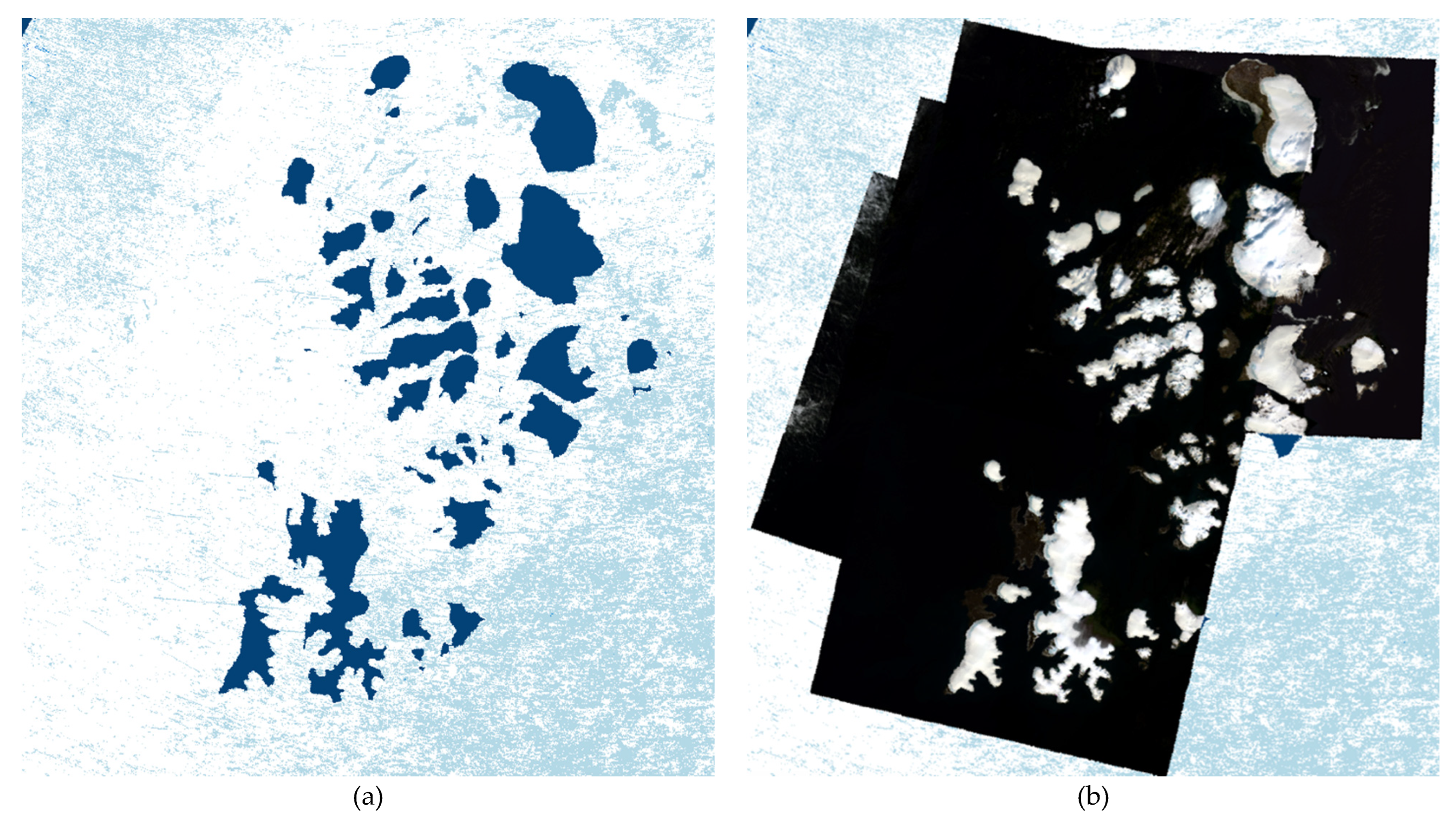
- (a)
- converts large amounts of MISR multiangular information into sea ice roughness images, and;
- (b)
- employs a new algorithm that converts the roughness images into geolocated and mosaicked maps of surface roughness over the entire Arctic.
2. Methods
2.1. Description of Data Sets
2.1.1. Airborne Topographic Mapper
2.1.2. Multi-Angle Imaging SpectroRadiometer (MISR)
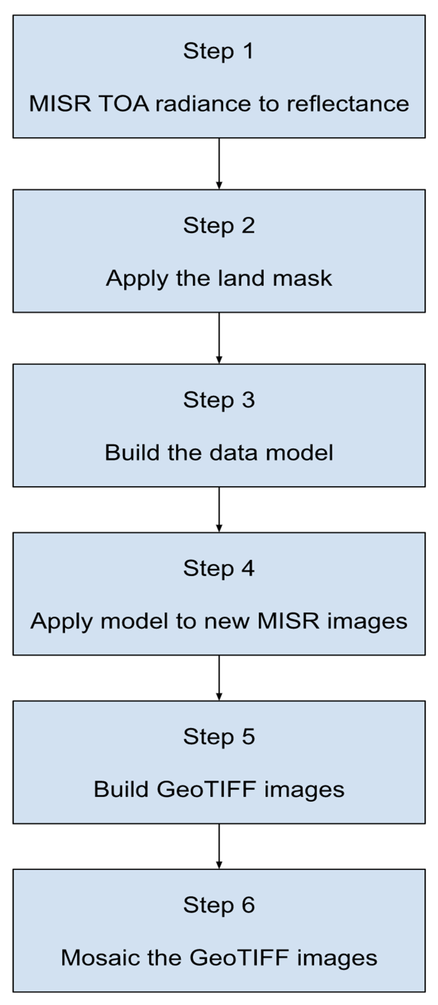
2.2. Data Preparation and Processing Steps
3. Results
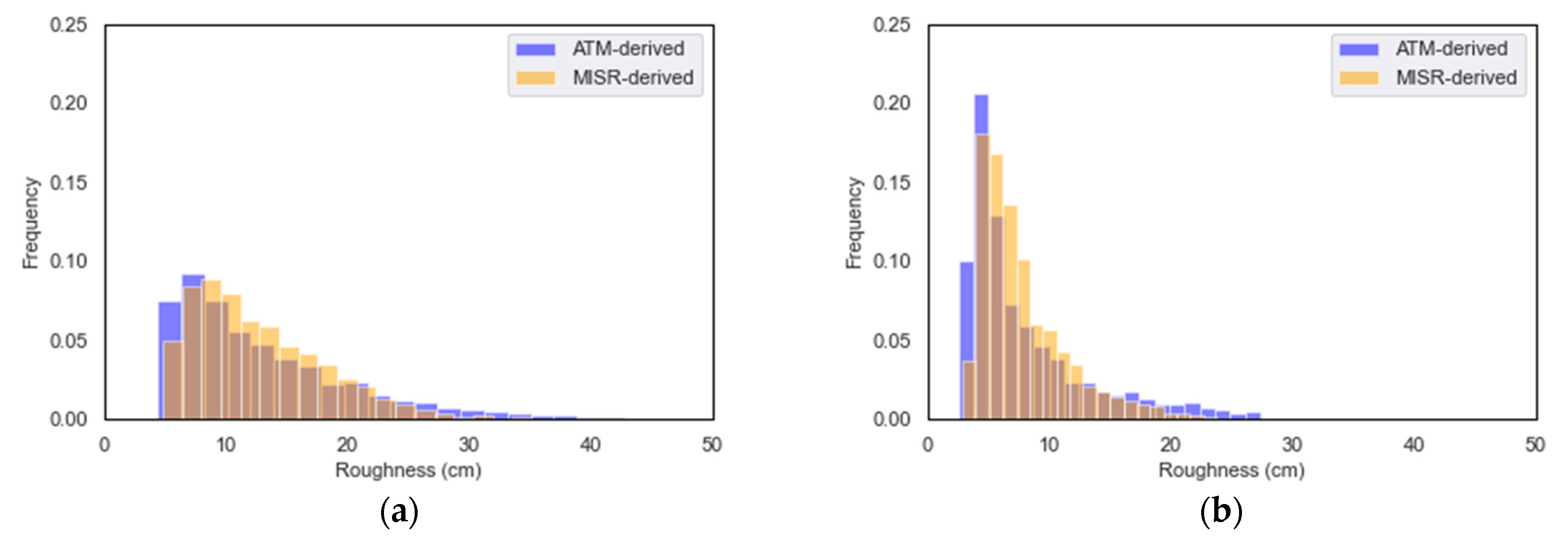
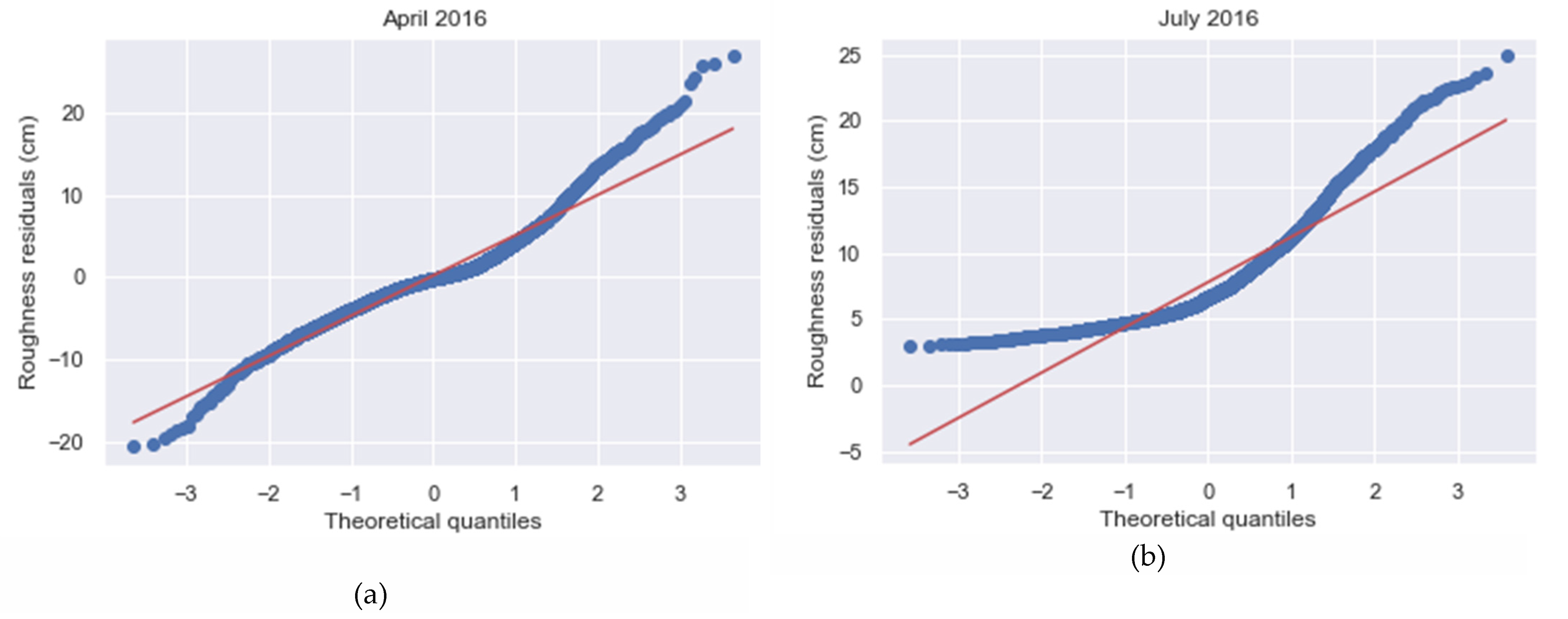
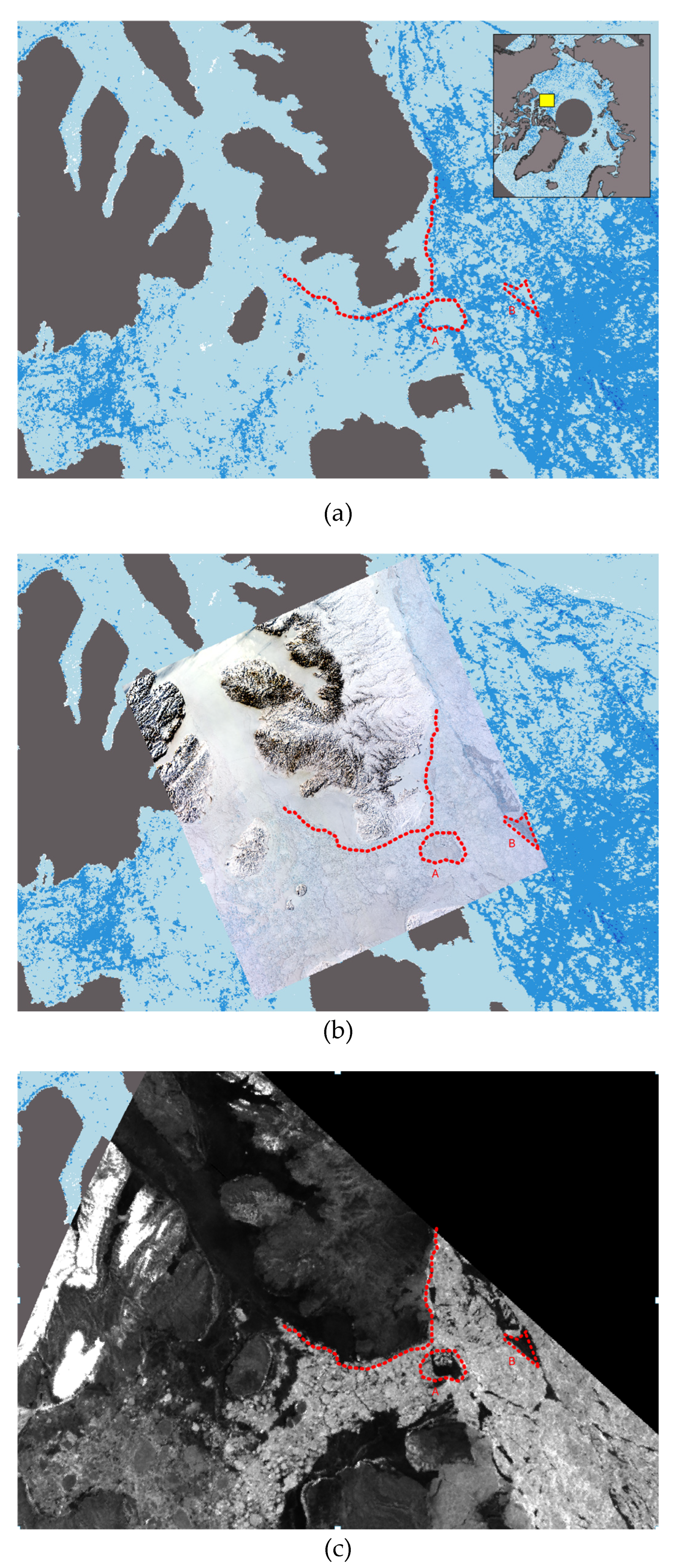
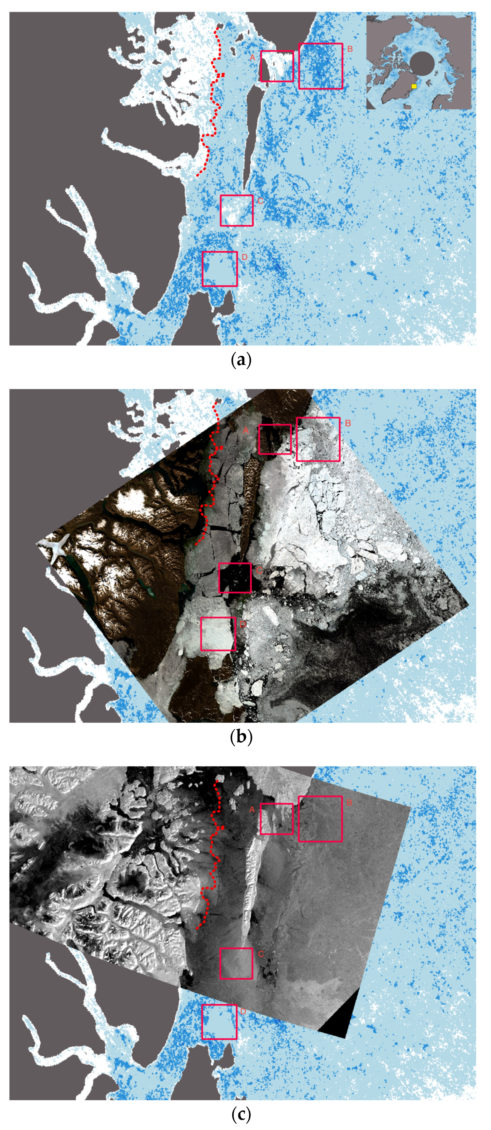
3.1. Evaluating Model Performance
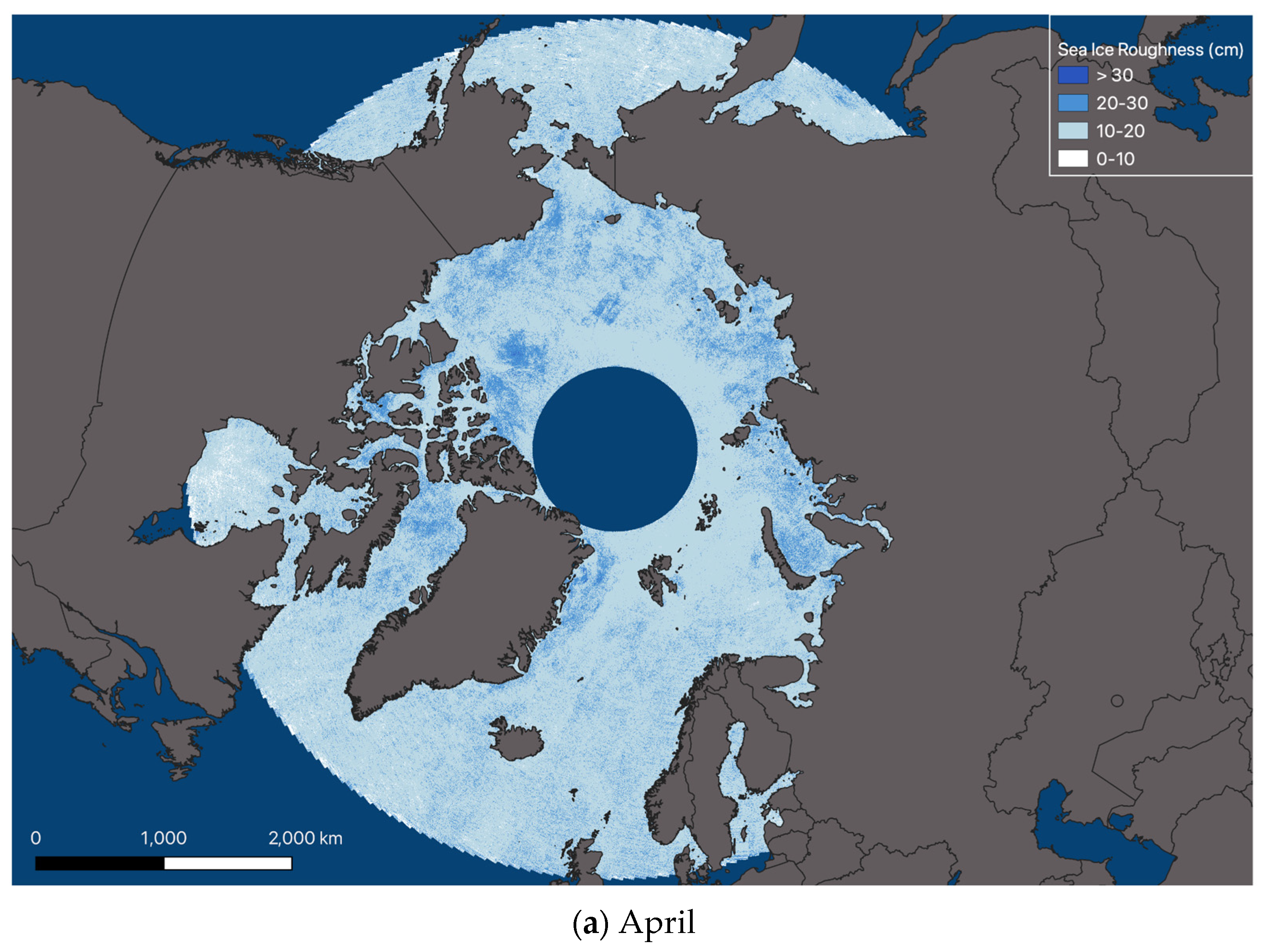
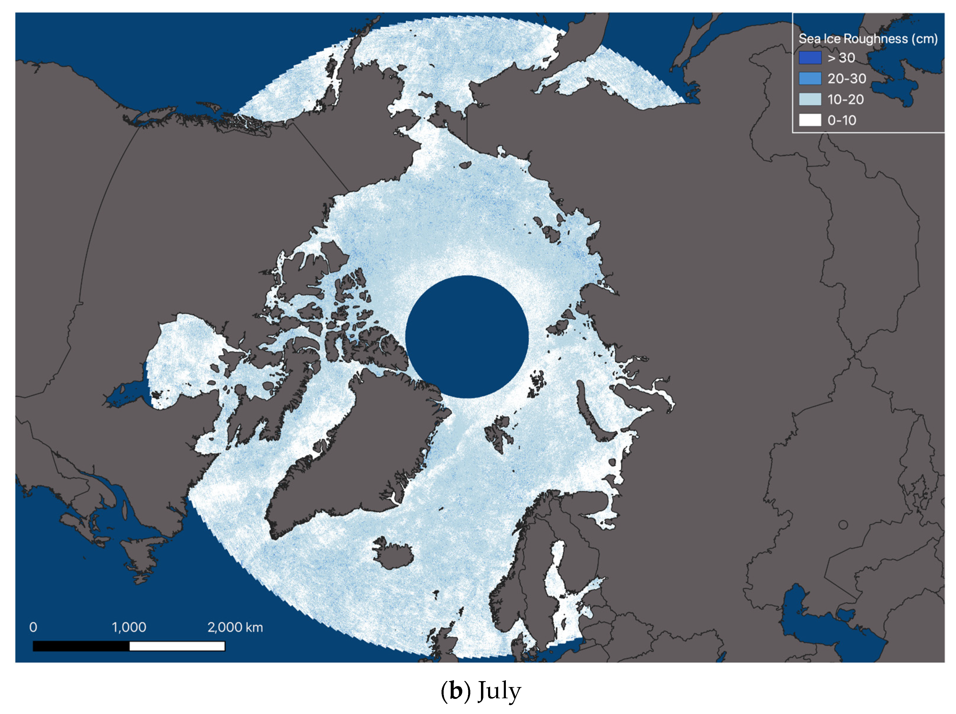
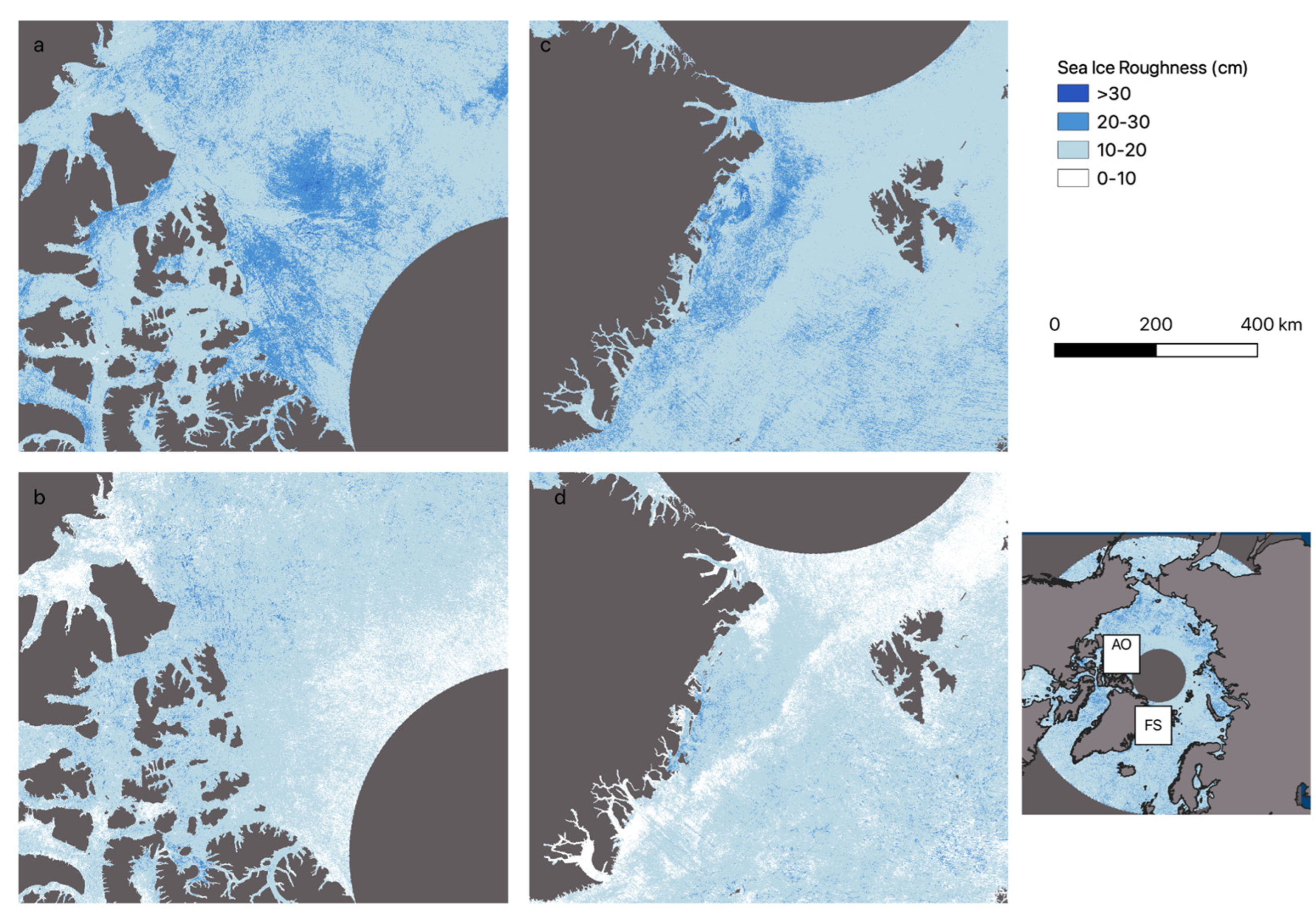
3.2. Spatial Patterns of Arctic Sea Ice Roughness
4. Discussion
5. Conclusions
Author Contributions
Funding
Institutional Review Board Statement
Informed Consent Statement
Data Availability Statement
Acknowledgments
Conflicts of Interest
References
- Rantanen, M.; Karpechko, A.Y.; Lipponen, A.; Nordling, K.; Hyvärinen, O.; Ruosteenoja, K.; Vihma, T.; Laaksonen, A. The Arctic Has Warmed Nearly Four Times Faster than the Globe since 1979. Commun. Earth Environ. 2022, 3, 168. [Google Scholar] [CrossRef]
- Holland, M.M.; Bitz, C.M.; Tremblay, B. Future Abrupt Reductions in the Summer Arctic Sea Ice. Geophys. Res. Lett. 2006, 33, 1–5. [Google Scholar] [CrossRef]
- Kumar, A.; Yadav, J.; Mohan, R. Global Warming Leading to Alarming Recession of the Arctic Sea-Ice Cover: Insights from Remote Sensing Observations and Model Reanalysis. Heliyon 2020, 6, e04355. [Google Scholar] [CrossRef]
- Meier, W.N.; Hovelsrud, G.K.; van Oort, B.E.H.; Key, J.R.; Kovacs, K.M.; Michel, C.; Haas, C.; Granskog, M.A.; Gerland, S.; Perovich, D.K.; et al. Arctic Sea Ice in Transformation: A Review of Recent Observed Changes and Impacts on Biology and Human Activity. Rev. Geophys. 2014, 52, 185–217. [Google Scholar] [CrossRef]
- Mueller, B.L.; Gillett, N.P.; Monahan, A.H.; Zwiers, F.W. Attribution of Arctic Sea Ice Decline from 1953 to 2012 to Influences from Natural, Greenhouse Gas, and Anthropogenic Aerosol Forcing. J. Clim. 2018, 31, 7771–7787. [Google Scholar] [CrossRef]
- Notz, D.; Community, S. Arctic Sea Ice in CMIP6. Geophys. Res. Lett. 2020, 47, e2019GL086749. [Google Scholar] [CrossRef]
- Stroeve, J.; Notz, D. Insights on Past and Future Sea-Ice Evolution from Combining Observations and Models. Glob. Planet. Chang. 2015, 135, 119–132. [Google Scholar] [CrossRef]
- Kwok, R.; Rothrock, D.A. Decline in Arctic Sea Ice Thickness from Submarine and ICESat Records: 1958–2008. Geophys. Res. Lett. 2009, 36, 1–5. [Google Scholar] [CrossRef]
- Meier, W.N.; Stroeve, J.; Fetterer, F. Whither Arctic Sea Ice? A Clear Signal of Decline Regionally, Seasonally and Extending beyond the Satellite Record. Ann. Glaciol. 2007, 46, 428–434. [Google Scholar] [CrossRef]
- Stroeve, J.; Notz, D. Changing State of Arctic Sea Ice across All Seasons. Environ. Res. Lett. 2018, 13, 103001. [Google Scholar] [CrossRef]
- Cavalieri, D.J.; Parkinson, C.L.; Gloersen, P.; Comiso, J.C.; Zwally, H.J. Deriving Long-Term Time Series of Sea Ice Cover from Satellite Passive-Microwave Multisensor Data Sets. J. Geophys. Res. Ocean. 1999, 104, 15803–15814. [Google Scholar] [CrossRef]
- Comiso, J.C. A Rapidly Declining Perennial Sea Ice Cover in the Arctic. Geophys. Res. Lett. 2002, 29, 17-1–17-4. [Google Scholar] [CrossRef]
- Comiso, J.C.; Parkinson, C.L.; Gersten, R.; Stock, L. Accelerated Decline in the Arctic Sea Ice Cover. Geophys. Res. Lett. 2008, 35, 1–6. [Google Scholar] [CrossRef]
- Parkinson, C.L.; Cavalieri, D.J.; Gloersen, P.; Zwally, H.J.; Comiso, J.C. Arctic Sea Ice Extents, Areas, and Trends, 1978–1996. J. Geophys. Res. Ocean. 1999, 104, 20837–20856. [Google Scholar] [CrossRef]
- Serreze, M.C.; Maslanik, J.A.; Scambos, T.A.; Fetterer, F.; Stroeve, J.; Knowles, K.; Fowler, C.; Drobot, S.; Barry, R.G.; Haran, T.M. A Record Minimum Arctic Sea Ice Extent and Area in 2002. Geophys. Res. Lett. 2003, 30, 1–4. [Google Scholar] [CrossRef]
- Farrell, S.L.; Duncan, K.; Buckley, E.M.; Richter-Menge, J.; Li, R. Mapping Sea Ice Surface Topography in High Fidelity With ICESat-2. Geophys. Res. Lett. 2020, 47, e2020GL090708. [Google Scholar] [CrossRef]
- Kharbouche, S.; Muller, J.-P. Sea Ice Albedo from MISR and MODIS: Production, Validation, and Trend Analysis. Remote Sens. 2019, 11, 9. [Google Scholar] [CrossRef]
- Kwok, R.; Cunningham, G.F.; Wensnahan, M.; Rigor, I.; Zwally, H.J.; Yi, D. Thinning and Volume Loss of the Arctic Ocean Sea Ice Cover: 2003–2008. J. Geophys. Res. Ocean. 2009, 114, 1–16. [Google Scholar] [CrossRef]
- Landy, J.C.; Ehn, J.K.; Barber, D.G. Albedo Feedback Enhanced by Smoother Arctic Sea Ice. Geophys. Res. Lett. 2015, 42, 10714–10720. [Google Scholar] [CrossRef]
- Yi, D.; Zwally, H.J.; Sun, X. ICESat Measurement of Greenland Ice Sheet Surface Slope and Roughness. Ann. Glaciol. 2005, 42, 83–89. [Google Scholar] [CrossRef]
- Segal, R.A.; Scharien, R.K.; Cafarella, S.; Tedstone, A. Characterizing Winter Landfast Sea-Ice Surface Roughness in the Canadian Arctic Archipelago Using Sentinel-1 Synthetic Aperture Radar and the Multi-Angle Imaging SpectroRadiometer. Ann. Glaciol. 2020, 61, 284–298. [Google Scholar] [CrossRef]
- Andreas, E.L.; Horst, T.W.; Grachev, A.A.; Persson, P.O.G.; Fairall, C.W.; Guest, P.S.; Jordan, R.E. Parametrizing Turbulent Exchange over Summer Sea Ice and the Marginal Ice Zone. Q. J. R. Meteorol. Soc. 2010, 136, 927–943. [Google Scholar] [CrossRef]
- Arya, S. Contribution of Form Drag on Pressure Ridges to the Air Stress on Arctic Ice. J. Geophys. Res. 1973, 78, 7092–7099. [Google Scholar] [CrossRef]
- Petty, A.A.; Tsamados, M.C.; Kurtz, N.T. Atmospheric Form Drag Coefficients over Arctic Sea Ice Using Remotely Sensed Ice Topography Data, Spring 2009-2015: Atmospheric Drag over Arctic Sea Ice. J. Geophys. Res. Earth Surf. 2017, 122, 1472–1490. [Google Scholar] [CrossRef]
- Steiner, N.; Harder, M.; Lemke, P. Sea-Ice Roughness and Drag Coefficients in a Dynamic–Thermodynamic Sea-Ice Model for the Arctic. Tellus Dyn. Meteorol. Oceanogr. 1999, 51, 964–978. [Google Scholar] [CrossRef]
- Arya, S.P.S. A Drag Partition Theory for Determining the Large-Scale Roughness Parameter and Wind Stress on the Arctic Pack Ice. J. Geophys. Res. 1975, 80, 3447–3454. [Google Scholar] [CrossRef]
- Castellani, G.; Lüpkes, C.; Hendricks, S.; Gerdes, R. Variability of Arctic Sea-Ice Topography and Its Impact on the Atmospheric Surface Drag. J. Geophys. Res. Ocean. 2014, 119, 6743–6762. [Google Scholar] [CrossRef]
- Guest, P.S.; Davidson, K.L. The Aerodynamic Roughness of Different Types of Sea Ice. J. Geophys. Res. Ocean. 1991, 96, 4709–4721. [Google Scholar] [CrossRef]
- Lüpkes, C.; Gryanik, V.M.; Rösel, A.; Birnbaum, G.; Kaleschke, L. Effect of Sea Ice Morphology during Arctic Summer on Atmospheric Drag Coefficients Used in Climate Models. Geophys. Res. Lett. 2013, 40, 446–451. [Google Scholar] [CrossRef]
- Lüpkes, C.; Gryanik, V.M.; Hartmann, J.; Andreas, E.L. A Parametrization, Based on Sea Ice Morphology, of the Neutral Atmospheric Drag Coefficients for Weather Prediction and Climate Models. J. Geophys. Res. Atmos. 2012, 117, 1–18. [Google Scholar] [CrossRef]
- Lei, R.; Tian-Kunze, X.; Leppäranta, M.; Wang, J.; Kaleschke, L.; Zhang, Z. Changes in Summer Sea Ice, Albedo, and Portioning of Surface Solar Radiation in the Pacific Sector of Arctic Ocean during 1982–2009. J. Geophys. Res. Ocean. 2016, 121, 5470–5486. [Google Scholar] [CrossRef]
- Lindsay, R.W.; Zhang, J. The Thinning of Arctic Sea Ice, 1988–2003: Have We Passed a Tipping Point? J. Clim. 2005, 18, 4879–4894. [Google Scholar] [CrossRef]
- Moritz, R.E.; Bitz, C.M.; Steig, E.J. Dynamics of Recent Climate Change in the Arctic. Science 2002, 297, 1497–1502. [Google Scholar] [CrossRef] [PubMed]
- Perovich, D.K.; Polashenski, C. Albedo Evolution of Seasonal Arctic Sea Ice: Aledo Evolution of Seasonal Sea Ice. Geophys. Res. Lett. 2012, 39, 1–6. [Google Scholar] [CrossRef]
- Stroeve, J.C.; Kattsov, V.; Barrett, A.; Serreze, M.; Pavlova, T.; Holland, M.; Meier, W.N. Trends in Arctic Sea Ice Extent from CMIP5, CMIP3 and Observations. Geophys. Res. Lett. 2012, 39, 1–7. [Google Scholar] [CrossRef]
- Zhang, J.; Rothrock, D.; Steele, M. Recent Changes in Arctic Sea Ice: The Interplay between Ice Dynamics and Thermodynamics. J. Clim. 2000, 13, 3099–3114. [Google Scholar] [CrossRef]
- Nolin, A.W.; Mar, E. Arctic Sea Ice Surface Roughness Estimated from Multi-Angular Reflectance Satellite Imagery. Remote Sens. 2019, 11, 50. [Google Scholar] [CrossRef]
- Nolin, A.W.; Fetterer, F.M.; Scambos, T.A. Surface Roughness Characterizations of Sea Ice and Ice Sheets: Case Studies with MISR Data. IEEE Trans. Geosci. Remote Sens. 2002, 40, 1605–1615. [Google Scholar] [CrossRef]
- Diner, D.J.; Asner, G.P.; Davies, R.; Knyazikhin, Y.; Muller, J.-P.; Nolin, A.W.; Pinty, B.; Schaaf, C.B.; Stroeve, J. New Directions in Earth Observing: Scientific Applications of Multiangle Remote Sensing. Bull. Am. Meteorol. Soc. 1999, 80, 2209–2228. [Google Scholar] [CrossRef]
- Nolin, A.W. Towards Retrieval of Forest Cover Density over Snow from the Multi-Angle Imaging SpectroRadiometer (MISR). Hydrol. Process. 2004, 18, 3623–3636. [Google Scholar] [CrossRef]
- Diner, D.J.; Beckert, J.C.; Reilly, T.H.; Bruegge, C.J.; Conel, J.E.; Kahn, R.A.; Martonchik, J.V.; Ackerman, T.P.; Davies, R.; Gerstl, S.A.W.; et al. Multi-Angle Imaging SpectroRadiometer (MISR) Instrument Description and Experiment Overview. IEEE Trans. Geosci. Remote Sens. 1998, 36, 1072–1087. [Google Scholar] [CrossRef]
- Studinger, M. 2014, Updated 2020. IceBridge ATM L2 Icessn Elevation, Slope, and Roughness, Version 2; NASA National Snow and Ice Data Center Distributed Active Archive Center: Boulder, CO, USA, 2014. [Google Scholar] [CrossRef]
- Brunt, K.M.; Hawley, R.L.; Lutz, E.R.; Studinger, M.; Sonntag, J.G.; Hofton, M.A.; Andrews, L.C.; Neumann, T.A. Assessment of NASA Airborne Laser Altimetry Data Using Ground-Based GPS Data near Summit Station, Greenland. Cryosphere 2017, 11, 681–692. [Google Scholar] [CrossRef]
- Kwok, R.; Kacimi, S.; Webster, M.A.; Kurtz, N.T.; Petty, A.A. Arctic Snow Depth and Sea Ice Thickness From ICESat-2 and CryoSat-2 Freeboards: A First Examination. J. Geophys. Res. Ocean. 2020, 125, e2019JC016008. [Google Scholar] [CrossRef]
- Kwok, R.; Cunningham, G.F. Variability of Arctic Sea Ice Thickness and Volume from CryoSat-2. Philos. Trans. R. Soc. Math. Phys. Eng. Sci. 2015, 373, 20140157. [Google Scholar] [CrossRef]
- Kwok, R.; Schweiger, A.; Rothrock, D.A.; Pang, S.; Kottmeier, C. Sea Ice Motion from Satellite Passive Microwave Imagery Assessed with ERS SAR and Buoy Motions. J. Geophys. Res. Ocean. 1998, 103, 8191–8214. [Google Scholar] [CrossRef]
- Min, C.; Mu, L.; Yang, Q.; Ricker, R.; Shi, Q.; Han, B.; Wu, R.; Liu, J. Sea Ice Export through the Fram Strait Derived from a Combined Model and Satellite Data Set. Cryosphere 2019, 13, 3209–3224. [Google Scholar] [CrossRef]
- Sea Ice Glossary-Woods Hole Oceanographic Institution. Available online: https://www.whoi.edu/ (accessed on 25 August 2022).


| SimpleLinearRegr | R2 | RMSE (cm) | MAE (cm) | MBE (cm) | ||||
|---|---|---|---|---|---|---|---|---|
| training | test | training | test | training | test | training | test | |
| April | 0.12 | 0.13 | 6.49 | 6.44 | 4.99 | 4.93 | 0 | −0.12 |
| July | 0.06 | 0.05 | 5 | 4.9 | 3.7 | 3.6 | 0 | −0.14 |
| PolyLinearRegr | R2 | RMSE (cm) | MAE (cm) | MBE (cm) | ||||
| training | test | training | test | training | test | training | test | |
| April | 0.28 | 0.29 | 5.87 | 5.8 | 4.45 | 4.36 | 0 | −0.15 |
| July | 0.11 | 0.09 | 4.77 | 4.84 | 3.56 | 3.6 | 0 | −0.09 |
| KNN | R2 | RMSE (cm) | MAE (cm) | MBE (cm) | ||||
| training | test | training | test | training | test | training | test | |
| April | 0.66 | 0.5 | 4.05 | 4.91 | 2.81 | 3.39 | −0.08 | −0.16 |
| July | 0.58 | 0.32 | 3.29 | 4.2 | 2.21 | 2.82 | −0.04 | −0.09 |
Publisher’s Note: MDPI stays neutral with regard to jurisdictional claims in published maps and institutional affiliations. |
© 2022 by the authors. Licensee MDPI, Basel, Switzerland. This article is an open access article distributed under the terms and conditions of the Creative Commons Attribution (CC BY) license (https://creativecommons.org/licenses/by/4.0/).
Share and Cite
Mosadegh, E.; Nolin, A.W. A New Data Processing System for Generating Sea Ice Surface Roughness Products from the Multi-Angle Imaging SpectroRadiometer (MISR) Imagery. Remote Sens. 2022, 14, 4979. https://doi.org/10.3390/rs14194979
Mosadegh E, Nolin AW. A New Data Processing System for Generating Sea Ice Surface Roughness Products from the Multi-Angle Imaging SpectroRadiometer (MISR) Imagery. Remote Sensing. 2022; 14(19):4979. https://doi.org/10.3390/rs14194979
Chicago/Turabian StyleMosadegh, Ehsan, and Anne W. Nolin. 2022. "A New Data Processing System for Generating Sea Ice Surface Roughness Products from the Multi-Angle Imaging SpectroRadiometer (MISR) Imagery" Remote Sensing 14, no. 19: 4979. https://doi.org/10.3390/rs14194979
APA StyleMosadegh, E., & Nolin, A. W. (2022). A New Data Processing System for Generating Sea Ice Surface Roughness Products from the Multi-Angle Imaging SpectroRadiometer (MISR) Imagery. Remote Sensing, 14(19), 4979. https://doi.org/10.3390/rs14194979