Stock Prediction Model Based on Mixed Fractional Brownian Motion and Improved Fractional-Order Particle Swarm Optimization Algorithm

Abstract

As one of the main areas of value investing, the stock market attracts the attention of many investors. Among investors, market index movements are a focus of attention. In this paper, combining the efficient market hypothesis and the fractal market hypothesis, a stock prediction model based on mixed fractional Brownian motion (MFBM) and an improved fractional-order particle swarm optimization algorithm is proposed. First, the MFBM model is constructed by adjusting the parameters to mix geometric Brownian motion (GBM) and geometric fractional Brownian motion (GFBM). After that, an improved fractional-order particle swarm optimization algorithm is proposed. The position and velocity formulas of the fractional-order particle swarm optimization algorithm are improved using new fractional-order update formulas. The inertia weight in the update formula is set to be linearly decreasing. The improved fractional-order particle swarm optimization algorithm is used to optimize the coefficients of the MFBM model. Through experiments, the accuracy and validity of the prediction model are proven by combining the error analysis. The model with the improved fractional-order particle swarm optimization algorithm and MFBM is superior to GBM, GFBM, and MFBM models in stock price prediction.

1. Introduction

Stock market investment, as one of the most profitable financial investments, is favored by many investors. The forecast of stock price movement has also been the focus of investors’ attention [1,2]. From the establishment of the stock market to date, research on market forecasting has never stopped [3]. There are many forecasting methods [4]. From the mathematical finance perspective, there are two main categories. One is the approach based on the efficient market hypothesis (EMH) [5,6] and the other is based on the fractal market hypothesis (FMH) [7].

In the 1970s, Fama [8,9] proposed the famous EMH based on the random wandering model. In EMH, the stock price trend follows the geometric Brownian motion (GBM) model [10]. EMH argued that every investor in the market was rational. Every stock price movement in the market is a comprehensive response to asset information. With prices following a random walk model, it is hard for investors receive a “free lunch” from the market. However, the efficient market hypothesis is only an ideal state and does not correspond to reality. Not every investor in the market has a rational mind and the information that occurs at each point in time is not fully embodied in the price. Some investors make good profits from the market. Therefore, many investors are skeptical of the efficient market hypothesis [11]. From the GBM model, GBM also has three conceptual errors. (1) For the GBM model, future changes are independent of past changes, which is not consistent with the fundamental characteristics of financial market development [12,13]. (2) The GBM model depicts a normal distribution, but real share prices have a “spike and a thick tail” [14]. (3) In stock prices, time series correlation is common everywhere [15]. That is to say, large decreases are usually accompanied by increases in volatility, while large increases are usually accompanied by decreases in volatility. Therefore, GBM cannot correctly describe the phenomenon and the laws of stock prices.

With further research, Peters [16] proposed the FMH from a nonlinear perspective and integrated fractal theory into financial markets. In FMH, stock price changes follow fractional Brownian motion (FBM) and yield obeys a fractal distribution characterized by self-similarity and long memory. FMH believes that the structure of the stock market is fractal and that it has a long memory [17]. The long memory is characterized by the Hurst value. In 2001, Wu pointed out that capital market price movements were mostly the fractal time series [18] and they explored the fractal dimension of stock prices using fractal and chaotic methods. However, Rostek [19,20] thought that there would be arbitrage in applying fractional Brownian motion to simulate prices under the fractal market assumption.

A better solution is to mix geometric Brownian motion and fractional Brownian motion. Then, mixed fractional Brownian motion (MFBM) is constructed to describe the process of asset price change [21]. In terms of the Hurst characteristic index, the standard Brownian motion is just a particular state of price fluctuations. For example, when the Hurst value is equal to 1/2, the fractional Brownian motion is converted to standard Brownian motion [22]. For another view of modern financial theory, the EMH and FMH are internally consistent, and the former is a special case of the latter. The EMH and FMH depict the linear and non-linear natures of financial markets. The fractal market is the general form and steady state of the securities market, while the effective market is the special form and biased state of the securities market. Therefore, the two theories have intrinsic uniformity. EMH reveals the ideal and special state of financial markets. FMH describes the volatility of market prices and the laws of market operation, and it provides a higher level of abstraction and description of financial fields [23]. The combination of EMH and FMH, that is, the combination of geometric and fractional Brownian to form MFBM, is the best model to describe asset price changes [24]. The market under the MFBM model not only has no arbitrage opportunity, but also is complete. It is more suitable for describing the operation and development of the market.

A perfectly efficient market describes the ideal state of financial markets. The most mature U.S. financial market is only between a weakly efficient market and a semi-strongly efficient market. For the Chinese stock market, the limit on ups and downs will keep the stock market in a relatively flat state, which satisfies the semi-strong EMH. In addition, the Chinese stock market is highly cyclical (long memory) [25]. Given these facts, this paper combines EMH and FMH. The price trends of the U.S. and Chinese stock markets are predicted through mixed fractional Brownian motion to obtain better forecasting results.

In this paper, we analyze stock price forms under the EMH and FMH. Then, MFBM is constructed by adjusting the parameters to mix GBM with FBM. The drift and diffusion coefficients in the MFBM model are solved by the maximum likelihood estimation (MLE) method. Then, the fractional-order particle swarm optimization algorithm is improved. The drift and diffusion coefficients of the MFBM are optimized by the improved fractional-order particle swarm optimization algorithm. Finally, the Hurst values are solved by the rescaled range (R/S) analysis method. The solved Hurst values are optimized by the improved fractional-order particle swarm optimization algorithm to find the optimal parameters and analyze the stock price prediction. Three market indices are selected for the Hurst solution and all results show that the three markets have long memory. The accuracy and validity of the prediction model are proven by combining the error analysis. The model with the improved fractional-order particle swarm optimization algorithm and MFBM is superior to GBM, GFBM, and MFBM in stock price prediction.

The main contributions of this paper are summarized as follows. (1) The parameters are adjusted to hybridize geometric and fractional Brownian motions. The MFBM model is constructed and used for stock market forecasting. (2) The fractional-order particle swarm optimization algorithm is improved. The MFBM model coefficients are optimized by the improved fractional-order particle swarm optimization algorithm. New variables are added to reduce the dependence of the update formula on the order of the fractional order. Both velocity and position formulas are derived for fractional order at the same time to improve the convergence speed. (3) The inertia weight factor in the improved fractional-order particle swarm optimization algorithm sets the linear decreasing principle in this paper. This reduces oscillations and increases the randomness of the particles. Therefore, the probability of the population falling into a local optimum is reduced.

The rest of this paper is organized as follows. Section 2 briefly introduces the generalized form of Brownian motion and constructs a stock price prediction model based on mixed fraction Brownian motion. In Section 3, the improvement process of the fractional-order particle swarm optimization algorithm is described in detail. Then, the parameters in the model are solved and optimized separately. In Section 4, three actual stock indices are selected to verify the validity of the IFPSO-MFBM methodology. The conclusion is given in Section 5.

2. MFBM Model

The MFBM model is constructed based on FBM and GBM. Then, some Brownian motion forms are briefly described.

2.1. Geometric Brownian Motion

Geometric Brownian motion is a stochastic equation of motion in continuous time. Since its trajectory is similar to the stock price trajectory, it is continuous but not derivable, with independent increments [26]. Therefore, it is often combined with the Black–Scholes model for stock price simulation in the field of financial mathematics. The stochastic process of GBM is determined by

$$\frac{\mathrm{dS}\left(\mathrm{t}\right)}{\mathrm{S}\left(\mathrm{t}\right)}=\mathsf{\mu }\mathrm{dt}+\mathsf{\sigma }\mathrm{dB}\left(\mathrm{t}\right),$$

(1)

where $\mathrm{S}\left(\mathrm{t}\right)$ represents the stock price. The $\frac{\mathrm{dS}\left(\mathrm{t}\right)}{\mathrm{S}\left(\mathrm{t}\right)}$ is the logarithmic return on the stock price and $\mathrm{B}\left(\mathrm{t}\right)$ is the standard Brownian motion (or Wiener process) obeying $\mathrm{N}\left(0,\mathrm{t}\right)$. The drift percentage μ and the volatility percentage σ are both constants. μ is the mathematical expectation of the asset price return. σ is the standard deviation of the asset price return.

From an economic point, Equation (1) can be interpreted using the Itô form stochastic equation, whose solution can be written as a geometric (economic) Brownian motion defined by

$${\mathrm{S}}_{\mathrm{t}}={\mathrm{S}}_0\exp \left\{\mathsf{\sigma }\mathrm{B}\left(\mathrm{t}\right)+\left(\mathsf{\mu }-\frac{{\mathsf{\sigma }}^2}{2}\right)\mathrm{t}\right\},$$

(2)

where ${\mathrm{S}}_{\mathrm{t}}$ is the stock price at time t and ${\mathrm{S}}_0$ is the initial share price.

Although the B–S pricing model is based on the geometric Brownian motion, the geometric Brownian motion describes share prices that are only appropriate for strong efficient markets. No market currently has strong efficient market conditions, so the geometric Brownian motion does not describe real market share prices.

2.2. Fractional Brownian Motion

Fractional Brownian motion is a derivative form of Brownian motion in the fractal market. There are two main differences between fractional Brownian motion and Brownian motion. One is that increments in fractional Brownian motion are not independent, whereas increments in Brownian motion are independent. The other difference is the dimensional value [27]. Fractional Brownian motion (fractal noise) has a fractional dimensional value. The value is equal to $1/\mathrm{H}$; here, $\mathrm{H}$ is the Hurst exponent [28]. Brownian motion (white noise) has a fractional dimensional value of 2. The above properties of fractional Brownian motion make it a suitable tool for mathematical finance. The formula for the covariance function of the FBM is determined by

$$\mathrm{E}\left[{\mathrm{B}}^{\mathrm{H}}\left(\mathrm{t}\right){\mathrm{B}}^{\mathrm{H}}\left(\mathrm{s}\right)\right]=\frac{1}{2}\left(|\mathrm{t}{|}^{2\mathrm{H}}+|\mathrm{s}{|}^{2\mathrm{H}}-|\mathrm{t}-\mathrm{s}{|}^{2\mathrm{H}}\right),$$

(3)

The stochastic process of geometric FBM is as follows:

$$\mathrm{dS}\left(\mathrm{t}\right)=\mathsf{\mu }\left(\mathrm{t}\right)\mathrm{S}\left(\mathrm{t}\right)\mathrm{dt}+\mathsf{\sigma }\mathrm{S}\left(\mathrm{t}\right){\mathrm{dB}}^{\mathrm{H}}\left(\mathrm{t}\right),$$

(4)

where ${\mathrm{B}}^{\mathrm{H}}$ is the fractional Brownian motion. The share price is based on (5) as follows:

$$\mathrm{S}\left(\mathrm{t}\right)={\mathrm{S}}_0\exp \left({\mathsf{\sigma }\mathrm{B}}^{\mathrm{H}}\left(\mathrm{t}\right)+\mathsf{\mu }\mathrm{t}-\frac{1}{2}{\mathsf{\sigma }}^2{\mathrm{t}}^{2\mathrm{H}}\right),$$

(5)

Fractional Brownian motion has long memory and is useful for financial market forecasting. Theoretically, there would be arbitrage in the model with FBM as the logarithmic price. In particular, it has been shown that arbitrage opportunities exist when trading in continuous or in discrete time [29,30].

2.3. Mixed Fractional Brownian Motion

Based on the intrinsic consistency of the EMH and FMH, a mixed fractional Brownian motion is constructed by adjusting the parameters to hybridize the geometric Brownian motion with the geometric fractional Brownian motion. The stochastic process of MFBM is determined by

$$\mathrm{dS}\left(\mathrm{t}\right)=\mathsf{\mu }\left(\mathrm{t}\right)\mathrm{S}\left(\mathrm{t}\right)\mathrm{dt}+\mathsf{\sigma }\mathrm{S}\left(\mathrm{t}\right){\mathrm{dW}}^{\mathrm{H}}\left(\mathrm{t}\right),$$

(6)

$${\mathrm{dW}}^{\mathrm{H}}\left(\mathrm{t}\right)={\mathsf{\rho }\mathrm{dB}}^{\mathrm{H}}\left(\mathrm{t}\right)+\left(1-\mathsf{\rho }\right)\mathrm{dB}\left(\mathrm{t}\right), \mathsf{\rho }\in \left(0,1\right),$$

(7)

where $\mathsf{\rho }$ is the mixing factor to be adjusted. The drift percentage μ and the volatility percentage σ are both constants. The $\mathrm{B}\left(\mathrm{t}\right)\left(\mathrm{t}\in {\mathrm{R}}^{+}\right)$ is a standard Brownian motion. The ${\mathrm{B}}^{\mathrm{H}}\left(\mathrm{t}\right)\left(\mathrm{t}\in {\mathrm{R}}^{+}\right)$ is a fractional Brownian motion with a Hurst value of H. These are independent of each other. The share price form is as follows:

$${\mathrm{S}}_{\mathrm{t}}={\mathrm{S}}_0\exp \{ \mathsf{\mu }\mathrm{t}+{\mathsf{\sigma }\mathrm{W}}^{\mathrm{H}}\left(\mathrm{t}\right)\},$$

(8)

which converts to Itô form as follows:

$${\mathrm{S}}_{\mathrm{t}}={\mathrm{S}}_0\exp \{\mathsf{\mu }\mathrm{t}+{\mathsf{\sigma }\mathrm{W}}^{\mathrm{H}}\left(\mathrm{t}\right)-\frac{1}{2}{\mathsf{\sigma }}^2{\mathsf{\rho }}^2{\mathrm{t}}^{2\mathrm{H}}-\frac{1}{2}{\mathsf{\sigma }}^2{\left(1-\mathsf{\rho }\right)}^2\mathrm{t}\},$$

(9)

In the MFBM model, the solution process of ${\mathrm{B}}^{\mathrm{H}}\left(\mathrm{t}\right)$ is as follows:

$${\mathrm{B}}^{\mathrm{H}}(\mathrm{t})={\int }_{\mathrm{t}}^0{\mathrm{K}}_{\mathrm{H}}(\mathrm{t},\mathrm{s})\mathrm{d}\mathrm{B}(\mathrm{s}),$$

(10)

$${\mathrm{K}}_{\mathrm{H}}(\mathrm{t},\mathrm{s})=\mathrm{c}(\mathrm{H})\frac{1}{{\mathrm{s}}^{\mathrm{H}-\frac{1}{2}}}{\int }_{\mathrm{t}}^{\mathrm{s}}\frac{{\mathrm{u}}^{\mathrm{H}-\frac{1}{2}}}{{\mathrm{u}-\mathrm{s}}^{\frac{3}{2}-\mathrm{H}}}\mathrm{d}\mathrm{u},$$

(11)

$$\mathrm{c}\left(\mathrm{H}\right)=\sqrt{\frac{2\mathrm{H}\Gamma \left(\frac{3}{2}-\mathrm{H}\right)}{\Gamma \left(\mathrm{H}+\frac{1}{2}\right)\Gamma (2-2\mathrm{H})}}(\mathrm{H}-\frac{1}{2}),$$

(12)

In (12), ${\mathrm{K}}_{\mathrm{H}}\left(\mathrm{t},\mathrm{s}\right)$ is a definite kernel, $\mathrm{c}\left(\mathrm{H}\right)$ is the normalization constant, and $\Gamma$ is the Gamma function, which can be solved according to Euler’s residue formula. The definition of the Gamma function over the real number field is defined by

$$\Gamma (\mathrm{x})={\int }_{\mathrm{0}}^{+\infty }{\mathrm{t}}^{\mathrm{x}-1}{\mathrm{e}}^{-\mathrm{t}}\mathrm{d}\mathrm{t}(\mathrm{x}>0),$$

(13)

Then, the ${\mathrm{B}}^{\mathrm{H}}\left(\mathrm{t}\right)$ value can be found here. The mixed fractional Brownian motion removes the arbitrage of fractional Brownian motion and retains its memorability [31]. It also combines the incremental and smooth characteristics of geometric Brownian motion.

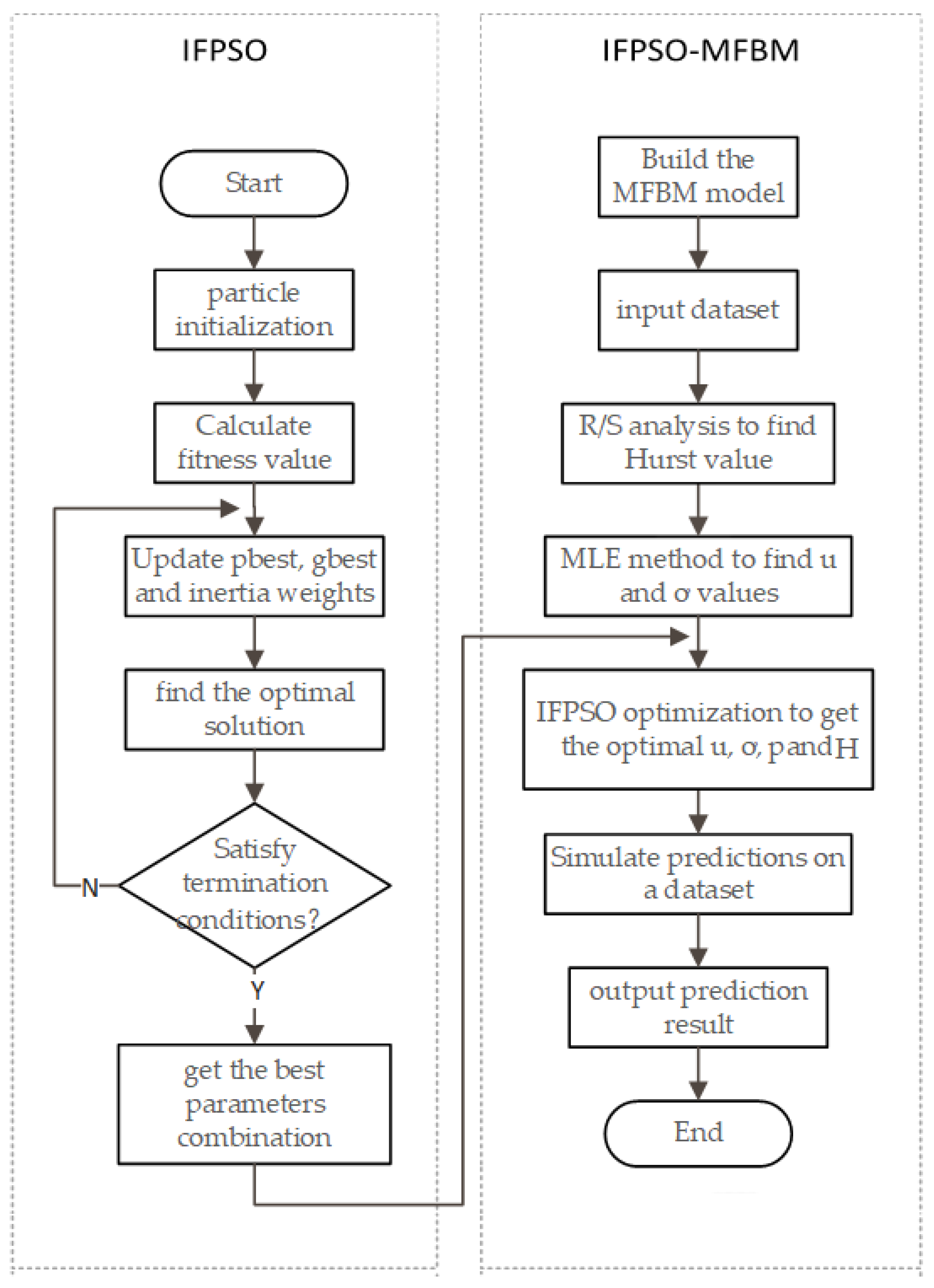
3. IFPSO-MFBM

The MFBM model that is constructed in the previous section contains a large number of parameters. Therefore, this section focuses on solving and optimizing the model parameters. Firstly, the fractional-order particle swarm optimization algorithm is improved. Hurst values in the model are then solved using rescaled range (R/S) analysis. Finally, the maximum likelihood estimate (MLE) method is used to find the drift and diffusion coefficients and the coefficients are further optimized using the improved fractional-order particle swarm optimization algorithm (IFPSO). The flow chart of stock index forecasting, based on the MFBM model and IFPSO algorithm, is shown in Figure 1.

3.1. Fractional-Particle Swarm Optimization Algorithm Improvement

The particle swarm optimization (PSO) algorithm originated from the simulation of the foraging behavior of birds [32]. The PSO algorithm is conceptually simple. It is easy to implement and converges quickly [33]. It is widely used to solve multi-objective optimization problems [34]. The standard PSO algorithm velocity and position formula are defined by

$${\mathrm{V}}_{\mathrm{id}}^{\mathrm{k}+1}=\mathrm{w}\times {\mathrm{V}}_{\mathrm{id}}^{\mathrm{k}}+{\mathrm{c}}_1\times {\mathrm{r}}_1\times \left({\mathrm{P}}_{\mathrm{id}}^{\mathrm{k}}-{\mathrm{X}}_{\mathrm{id}}^{\mathrm{k}}\right)+{\mathrm{c}}_2\times {\mathrm{r}}_2\times \left({\mathrm{P}}_{\mathrm{gd}}^{\mathrm{k}}-{\mathrm{X}}_{\mathrm{id}}^{\mathrm{k}}\right),$$

(14)

$${\mathrm{X}}_{\mathrm{id}}^{\mathrm{k}+1}={\mathrm{X}}_{\mathrm{id}}^{\mathrm{k}}+{\mathrm{V}}_{\mathrm{id}}^{\mathrm{k}+1},$$

(15)

where $\mathrm{k}$ is the number of iterations. ${ \mathrm{P}}_{\mathrm{id}}^{\mathrm{k}}$ is the particle position and ${\mathrm{V}}_{\mathrm{id}}^{\mathrm{k}}$ is the particle velocity. c₁ and c₂ are acceleration factors. r₁ and r₂ are random numbers distributed between (0, 1). $\mathrm{w}$ is the inertia weight factor. The weight update equation is computed by

$$\mathrm{w}\left(\mathrm{k}\right)={\mathrm{w}}_{\max }-\frac{\left({\mathrm{w}}_{\max }-{ \mathrm{w}}_{\min }\right)\ast \mathrm{k}}{{\mathrm{k}}_{\max }},$$

(16)

In the standard PSO algorithm, the particles converge slowly. Therefore, Pires [35] introduced fractional order calculus into PSO and proposed the fractional order particle swarm optimization (FOPSO) algorithm. The convergence speed of the algorithm is improved by introducing fractional order integration in the particle swarm velocity equation. However, the FOPSO algorithm is susceptible to falling into local solutions. When dealing with complex multi-peaked problems, the FOPSO algorithm tends to the local optimum. The convergence performance is directly dependent on the fractional order $\mathsf{\alpha }$. When the value of $\mathsf{\alpha }$ increases, the particles converge more slowly. When the value of $\mathsf{\alpha }$ decreases, the population tends to fall into a local optimum. In this paper, we improve the fractional-order algorithm. The velocity and position equations are derived by fractional order calculus simultaneously. The inertia weight factor w is set to be linearly decreasing to avoid falling into a local optimum.

When improving the PSO algorithm, the fractional order Grunwald–Letnikov (G–L) definition is used. Its $\mathsf{\alpha }$(R) order derivative is approximated in discrete time as follows:

$${\mathrm{D}}^{\mathsf{\alpha }}\mathrm{f}\left(\mathrm{x}\right)=\frac{1}{{\mathrm{T}}^{\mathrm{a}}}{{\displaystyle \sum }}_{\mathrm{k}=0}^{\mathrm{r}}\frac{{(-1)}^{\mathrm{k}}\Gamma \left(\mathsf{\alpha }+1\right)\mathrm{f}\left(\mathrm{x}-\mathrm{kh}\right)}{\Gamma \left(\mathrm{k}+1\right)\Gamma \left(\mathsf{\alpha }-\mathrm{k}+1\right)},$$

(17)

where T is the sampling period and $\Gamma$ is the Gamma function.

The PSO fractional order improvement process is as follows:

Step 1: A left-right transformation of the standard particle swarm algorithm is made; then, there is the following equation

$${\mathrm{V}}_{\mathrm{id}}^{\mathrm{k}+1}-{\mathrm{V}}_{\mathrm{id}}^{\mathrm{k}}=\left(\mathrm{w}-1\right)\times {\mathrm{V}}_{\mathrm{id}}^{\mathrm{k}}+{\mathrm{c}}_1\times {\mathrm{r}}_1\times \left({\mathrm{P}}_{\mathrm{id}}^{\mathrm{k}}-{\mathrm{X}}_{\mathrm{id}}^{\mathrm{k}}\right)+{\mathrm{c}}_2\times {\mathrm{r}}_2\times \left({\mathrm{P}}_{\mathrm{gd}}^{\mathrm{k}}-{\mathrm{X}}_{\mathrm{id}}^{\mathrm{k}}\right),$$

(18)

where ${\mathrm{V}}_{\mathrm{id}}^{\mathrm{k}+1}-{\mathrm{V}}_{\mathrm{id}}^{\mathrm{k}}$ is the derivative of the discrete state at fractional order $\mathsf{\alpha }$ = 1;

Step 2: Assuming a sampling period T = 1, followed by a generalization of Equation (18) to fractional order differentiation:

$${\mathrm{D}}^{\mathrm{a}}\left[{\mathrm{V}}_{\mathrm{id}}^{\mathrm{k}+1}\right]=\left(\mathrm{w}-1\right)\times {\mathrm{V}}_{\mathrm{id}}^{\mathrm{k}}+{\mathrm{c}}_1\times {\mathrm{r}}_1\times \left({\mathrm{P}}_{\mathrm{id}}^{\mathrm{k}}-{\mathrm{X}}_{\mathrm{id}}^{\mathrm{k}}\right)+{\mathrm{c}}_2\times {\mathrm{r}}_2\times \left({\mathrm{P}}_{\mathrm{gd}}^{\mathrm{k}}-{\mathrm{X}}_{\mathrm{id}}^{\mathrm{k}}\right);$$

(19)

Step 3: Considering the decreasing relationship between the number of contemporary particles and the number of particles of previous generations, Equation (19) is kept for only the first four generations of vectors owing to the memory property of fractional order calculus. The velocity formulation of the particle swarm algorithm is extended from first order to arbitrary order through the fractional order G-L definition.

$${\mathrm{D}}^{\mathrm{a}}\left[{\mathrm{V}}_{\mathrm{id}}^{\mathrm{k}+1}\right]={\mathrm{V}}_{\mathrm{id}}^{\mathrm{k}+1}-{\mathrm{aV}}_{\mathrm{id}}^{\mathrm{k}}-\frac{1}{2}\mathrm{a}\left(1-\mathrm{a}\right){\mathrm{V}}_{\mathrm{id}}^{\left(\mathrm{k}-1\right)}-\frac{1}{6}\mathrm{a}\left(1-\mathrm{a}\right)\left(2-\mathrm{a}\right){\mathrm{V}}_{\mathrm{id}}^{\left(\mathrm{k}-2\right)}-\frac{1}{24}\mathrm{a}\left(1-\mathrm{a}\right)\left(2-\mathrm{a}\right)\left(3-\mathrm{a}\right){\mathrm{V}}_{\mathrm{id}}^{\left(\mathrm{k}-3\right)};$$

(20)

Step 4: Combining (19) and (20), the final velocity equation of the fractional-order particle swarm algorithm with linearly decreasing weight coefficients is obtained

$$\begin{array}{c}{\mathrm{V}}_{\mathrm{id}}^{\mathrm{k}+1}=(\mathrm{w}-1+\mathrm{a}){\mathrm{V}}_{\mathrm{id}}^{\mathrm{k}}+\frac{1}{2}\mathrm{a}\left(1-\mathrm{a}\right){\mathrm{V}}_{\mathrm{id}}^{\left(\mathrm{k}-1\right)}-\frac{1}{6}\mathrm{a}\left(1-\mathrm{a}\right)\left(2-\mathrm{a}\right){\mathrm{V}}_{\mathrm{id}}^{\left(\mathrm{k}-2\right)}+\hfill \\ \frac{1}{24}\mathrm{a}\left(1-\mathrm{a}\right)\left(2-\mathrm{a}\right)\left(3-\mathrm{a}\right){\mathrm{V}}_{\mathrm{id}}^{\left(\mathrm{k}-3\right)}+{\mathrm{c}}_1\times {\mathrm{r}}_1\times \left({\mathrm{P}}_{\mathrm{id}}^{\mathrm{k}}-{\mathrm{X}}_{\mathrm{id}}^{\mathrm{k}}\right)+{\mathrm{c}}_2\times {\mathrm{r}}_2\times \left({\mathrm{P}}_{\mathrm{gd}}^{\mathrm{k}}-{\mathrm{X}}_{\mathrm{id}}^{\mathrm{k}}\right),\hfill \end{array}$$

(21)

By introducing fractional order differential operators, the current particle swarm algorithm is made to relate to the particle velocities of previous stages. Therefore, the algorithm is made to have a memory function;

Step 5: Then, the same fractional-order improvement is performed for the position update. The position updating formula of the fractional order particle swarm algorithm with linearly decreasing weight coefficients is obtained:

$${\mathrm{X}}_{\mathrm{id}}^{\mathrm{k}+1}=(\mathrm{w}-1+\mathrm{a}){\mathrm{V}}_{\mathrm{id}}^{\mathrm{k}}+\frac{1}{2}\mathrm{a}\left(1-\mathrm{a}\right){\mathrm{V}}_{\mathrm{id}}^{\left(\mathrm{k}-1\right)}-\frac{1}{6}\mathrm{a}\left(1-\mathrm{a}\right)\left(2-\mathrm{a}\right){\mathrm{V}}_{\mathrm{id}}^{\left(\mathrm{k}-2\right)}+\frac{1}{24}\mathrm{a}\left(1-\mathrm{a}\right)\left(2-\mathrm{a}\right)\left(3-\mathrm{a}\right){\mathrm{V}}_{\mathrm{id}}^{\left(\mathrm{k}-3\right)}+{\mathrm{c}}_1\times {\mathrm{r}}_1\times \left({\mathrm{P}}_{\mathrm{id}}^{\mathrm{k}}-{\mathrm{X}}_{\mathrm{id}}^{\mathrm{k}}\right)+{\mathrm{c}}_2\times {\mathrm{r}}_2\times \left({\mathrm{P}}_{\mathrm{gd}}^{\mathrm{k}}-{\mathrm{X}}_{\mathrm{id}}^{\mathrm{k}}\right)+\mathsf{\beta }{\mathrm{X}}_{\mathrm{id}}^{\mathrm{k}}+\frac{1}{2}\mathsf{\beta }\left(1-\mathsf{\beta }\right){\mathrm{X}}_{\mathrm{id}}^{\mathrm{k}-1}+\frac{1}{6}\mathsf{\beta }\left(1-\mathsf{\beta }\right)\left(2-\mathsf{\beta }\right){\mathrm{X}}_{\mathrm{id}}^{\mathrm{k}-2}$$

(22)

The positions of the particles of the improved fractional-order particle swarm algorithm (IFPSO) are no longer only influenced by the fractional order $\mathsf{\alpha }$. The introduction of fractional order $\mathsf{\beta }$ allows the position update to be associated with the previous position.

The IFPSO offers significant improvements in convergence speed, stability, and accuracy, and further enhances the ability to find globally optimal solutions.

3.2. R/S Analysis for Hurst Index

When Hurst (the British hydrologist) studied the relationship between water flow and storage capacity in the Nile reservoir, he found that the relationship could be better described in terms of fractal Brownian motion [36]. He then proposed the Hurst index. There are several methods for solving the Hurst exponent [37]. The earliest method proposed by scholars in the time domain is the R/S estimation method. After that, wavelet analysis, the variance method, and the mean value method were gradually derived [38]. This paper focuses on solving Hurst values using R/S analysis. The process is as follows:

• Let a time series ${\left\{{\mathrm{x}}_{\mathrm{t}}\right\}}_{\mathrm{t}}^{\mathrm{M}}=1$, of length $\mathrm{M}$, be divided into $\mathrm{N}$ adjacent subintervals of length $\mid \frac{\mathrm{M}}{\mathrm{N}}\mid$;
• For the subintervals, let the sample mean be ${\mathrm{e}}_{\mathrm{u}}=\frac{1}{\mathrm{N}}{\sum }_{\mathrm{i}=1}^{\mathrm{N}}{\mathrm{x}}_{\mathrm{i}}+(\mathrm{u}-1)\times \mathrm{N}(\mathrm{u}=1,2,\dots ,\mid \frac{\mathrm{M}}{\mathrm{N}}\mid )$;
• For a subinterval $\mathrm{u}$, take ${\mathrm{y}}_{\mathrm{u},\mathrm{i}}={\mathrm{x}}_{\mathrm{i}}+\left(\mathrm{u}-1\right)\times \mathrm{N}-{\mathrm{e}}_{\mathrm{u}}$(i = 1, 2,…, N) such that ${ \mathrm{z}}_{\mathrm{u},\mathrm{i}}={\sum }_{\mathrm{i}=1}^{\mathrm{N}}{\mathrm{y}}_{\mathrm{u},\mathrm{i}}$. The ${\mathrm{z}}_{\mathrm{u},\mathrm{i}}$ is the cumulative return. Here, u = 1, 2, …,$\mid \frac{\mathrm{M}}{\mathrm{N}}\mid$;
• Calculate ${\mathrm{R}}_{\mathrm{u}}={\max }_{1\le \mathrm{N}\le \mathrm{N}}{\mathrm{Z}}_{\mathrm{u},\mathrm{i}}-{\min }_{1\le \mathrm{i}\le \mathrm{N}}{\mathrm{Z}}_{\mathrm{u},\mathrm{i}}$ as the extreme deviation of the subinterval u. Let ${\mathrm{S}}_{\mathrm{u}}$ be the standard deviation of the cumulative return for the interval;
• Calculate the rescaled polar difference ${\mathrm{R}}_{\mathrm{u}}/{\mathrm{S}}_{\mathrm{u}}$ for each interval; $\mid \frac{\mathrm{M}}{\mathrm{N}}\mid$ intervals can obtain $\mid \frac{\mathrm{M}}{\mathrm{N}}\mid$ values (u = 1, 2, …). Take its mean value ${\mathrm{R}}_{\mathrm{N}}/{\mathrm{S}}_{\mathrm{N}}$ as the rescaled polar deviation value for an interval of length N;
• Taking the logarithm of both ends of the ${\mathrm{R}}_{\mathrm{N}}/{\mathrm{S}}_{\mathrm{N}}={\mathrm{bN}}^{\mathrm{H}}$ equation yields: $\log ({\mathrm{R}}_{\mathrm{N}}/{\mathrm{S}}_{\mathrm{N}})$=$\mathrm{HlogN}+\mathrm{logby}\left(\mathrm{n}\right)$; b is a constant and H is the Hurst index;
• Repeat Steps 1 to 6 for different interval lengths N to obtain different values of ${\mathrm{R}}_{\mathrm{N}}/{\mathrm{S}}_{\mathrm{N}}$. By regression analysis, the slope is the desired H value.

Given a time series ${\mathrm{X}}_{\mathrm{i}}, \mathrm{i}=1,2,\dots , \mathrm{N}$, calculate the sum of the partial series as $\mathrm{y}\left(\mathrm{n}\right)={\sum }_{\mathrm{i}=1}^{\mathrm{n}}{\mathrm{X}}_{\mathrm{i}}$ and define the sample variance as ${\mathrm{S}}^2\left(\mathrm{n}\right)$; then, one obtains the formula:

$${\mathrm{S}}^2\left(\mathrm{n}\right)=\frac{1}{\mathrm{n}}{\sum }_{\mathrm{i}=1}^{\mathrm{n}}{\mathrm{X}}_{\mathrm{i}}^2-\frac{1}{{\mathrm{n}}^2}{\mathrm{y}}^2\left(\mathrm{n}\right),$$

(23)

The final R/S is calculated by

$$\frac{\mathrm{R}}{\mathrm{S}}\left(\mathrm{n}\right)=\frac{1}{\mathrm{S}\left(\mathrm{n}\right)}\left[{\max }_{0\le \mathrm{t}\le \mathrm{n}}\left(\mathrm{y}\left(\mathrm{t}\right)-\frac{\mathrm{t}}{\mathrm{n}}\mathrm{y}\left(\mathrm{t}\right)\right)-{\min }_{0\le \mathrm{t}\le \mathrm{n}}\left(\mathrm{y}\left(\mathrm{t}\right)-\frac{\mathrm{t}}{\mathrm{n}}\mathrm{y}\left(\mathrm{t}\right)\right)\right],$$

(24)

When $\mathrm{n}\to \infty$,$\mathrm{E}\left[\mathrm{R}/\mathrm{S}\left(\mathrm{n}\right)\right]\sim {\mathrm{C}}_{\mathrm{H}}{\mathrm{n}}^{\mathrm{H}}$, ${\mathrm{C}}_{\mathrm{H}}$ is a constant positive constant, taking the logarithm of the above Equation (24). A log–log plot is drawn and a straight line is fitted using least squares regression. The slope of this line is calculated as the Hurst index value for a given time series.

3.3. MLE Method for the Drift Coefficient $\mu$ and the Diffusion Coefficient $\sigma$

The MLE method [39] is chosen to estimate the parameters σ and µ in this paper. According to the solution of ordinary differential equations, take the logarithm of the left and right sides of Equation (9) to obtain:

$$\ln \left({\mathrm{S}}_{\mathrm{t}}\right)-\ln ({\mathrm{S}}_0)=\mathsf{\mu }\mathrm{t}+{\mathsf{\sigma }\mathrm{W}}_{\mathrm{t}}^{\mathrm{H}},$$

(25)

Thus, the parameter estimate for Equation (25) is equivalent:

$${\mathrm{Y}}_{\mathrm{t}}=\mathsf{\mu }\mathrm{t}+{\mathsf{\sigma }\mathrm{W}}_{\mathrm{t}}^{\mathrm{H}}, \mathrm{t}\ge 0,$$

(26)

The time series observation interval is h. The vector $\mathrm{t}=\left(\mathrm{h},2\mathrm{h},\dots , \mathrm{Nh}\right)$ is used to represent the observation time point. The observation vectors $\mathrm{Y}=\left({\mathrm{Y}}_{\mathrm{h}},{ \mathrm{Y}}_{2\mathrm{h}},\dots ,{ \mathrm{Y}}_{\mathrm{Nh}}\right)$ are obtained. The MFBM process is ${\mathrm{W}}_{\mathrm{t}}^{\mathrm{H}}=\left({\mathrm{W}}_{\left(\mathrm{h}\right)}^{\mathrm{H}},{ \mathrm{W}}_{\left(2\mathrm{h}\right)}^{\mathrm{H}},\dots ,{ \mathrm{W}}_{\left(\mathrm{Nh}\right)}^{\mathrm{H}}\right)$. Then, the maximum likelihood estimates of the drift coefficient $\mathsf{\mu }$ and the diffusion coefficient $\mathsf{\sigma }$ are derived from the following steps.

According to the joint density of the multidimensional normal distribution, the MFBM model has the properties of a Gaussian process. Therefore, the observation vector Y obeys a multivariate normal distribution. Substitute Y into Equation (26) and then derive the specific expression for each covariance ${\mathsf{\sigma }}_{\mathrm{H}}^2$ in the discrete covariance matrix ${{\displaystyle \sum }}_{\mathrm{H}}$ based on (25) as follows:

$${\mathsf{\sigma }}_{\mathrm{H}}^2={\left[\mathrm{E}\left[{\mathrm{W}}_{\left(\mathrm{ih}\right)}^{\mathrm{H}},{\mathrm{W}}_{\left(\mathrm{jh}\right)}^{\mathrm{H}}\right]\right]}_{\mathrm{i},\mathrm{j}=1,2,\dots \mathrm{N}}=\frac{{\mathsf{\sigma }}^2}{2}{\mathrm{h}}^{2\mathrm{H}}{\left({\mathrm{i}}^{2\mathrm{H}}+{\mathrm{j}}^{2\mathrm{H}}-|\mathrm{i}-\mathrm{j}{|}^{2\mathrm{H}}\right)}_{\mathrm{i},\mathrm{j}=1,2,\dots \mathrm{N}},$$

(27)

The joint probability density function of the multidimensional normal distribution of Y is defined by

$$\mathrm{g}\left(\mathrm{Y}\right)={\left(2{\mathsf{\pi }\mathsf{\sigma }}^2\right)}^{-\frac{\mathrm{N}}{2}}{\left|{\Gamma }_{\mathrm{H}}\right|}^{-\frac{1}{2}}\exp \left(-\frac{1}{2{\mathsf{\sigma }}^2}{(\mathrm{Y}-\mathsf{\mu }\mathrm{t})}^{\prime }{\Gamma }_{\mathrm{H}}^{-1}\left(\mathrm{Y}-\mathsf{\mu }\mathrm{t}\right)\right),$$

(28)

where ${\Gamma }_{\mathrm{H}}=\frac{1}{2}{\mathrm{h}}^{2\mathrm{H}}{\left({\mathrm{i}}^{2\mathrm{H}}+{\mathrm{j}}^{2\mathrm{H}}-|\mathrm{i}-\mathrm{j}{|}^{2\mathrm{H}}\right)}_{\mathrm{i},\mathrm{j}=1,2,\dots ,\mathrm{N}}.$

Find the log-likelihood function for the joint probability density function:

$$\mathrm{lng}\left(\mathrm{Y}\right)=-\frac{\mathrm{N}}{2}\ln \left(2{\mathsf{\pi }\mathsf{\sigma }}^2\right)-\frac{1}{2}\ln \left|{\Gamma }_{\mathrm{H}}\right|-\frac{1}{2{\mathsf{\sigma }}^2}{(\mathrm{Y}-\mathsf{\mu }\mathrm{t})}^{\prime }{\Gamma }_{\mathrm{H}}^{-1}\left(\mathrm{Y}-\mathsf{\mu }\mathrm{t}\right),$$

(29)

Find the partial derivatives for μ and ${\mathsf{\sigma }}^2$ with respect to (26). Set the partial derivatives equal to 0.

The maximum likelihood estimate of the drift coefficient μ is obtained by taking the partial derivative of μ as:

$$\stackrel{`}{\mathsf{\mu }}=\frac{{ {\mathrm{t}}^{\prime }\Gamma }_{\mathrm{H}}^{-1}\mathrm{Y}}{{ {\mathrm{t}}^{\prime }\Gamma }_{\mathrm{H}}^{-1}{\mathrm{t}}^{\prime }},$$

(30)

Similarly, the maximum likelihood estimate for finding the partial derivative ${\mathsf{\sigma }}^2$ is as follows:

$${\stackrel{`}{\mathsf{\sigma }}}^2=\frac{1}{\mathrm{N}}\frac{\left({ {\mathrm{Y}}^{\prime }\Gamma }_{\mathrm{H}}^{-1}\mathrm{Y}\right)\left({ {\mathrm{t}}^{\prime }\Gamma }_{\mathrm{H}}^{-1}\mathrm{t}\right)-{\left({ {\mathrm{t}}^{\prime }\Gamma }_{\mathrm{H}}^{-1}\mathrm{Y}\right)}^2}{{ {\mathrm{t}}^{\prime }\Gamma }_{\mathrm{H}}^{-1}\mathrm{t}},$$

(31)

3.4. IFPOS Algorithm Optimizing σ, µ, ρ, and H

In this paper, σ, µ, ρ, and H are optimized by the improved fractional PSO algorithm in Section 3.1. The steps can be summarized as follows:

Step 1: The Hurst of the MFBM model is obtained from known stock market data and the unknown parameters are determined based on R/S analysis;

Step 2: Using the maximum likelihood estimation method, the drift coefficient σ and the diffusion coefficient µ are solved separately to obtain the original values of each parameter of the model;

Step 3: The IFPSO algorithm is used to continue the optimization of the model parameters. The individual extreme value of each particle is set to the current position. According to the weight update formula, the current inertia weight value is calculated and updated. The velocity and position of the particle are updated according to the improved particle velocity and position update formula;

Step 4: The updated fitness value of each particle is calculated according to the fitness function of the particle. The fitness value of each particle is compared with its individual extreme value. If the individual extreme value is better than the fitness value, the individual extreme value is updated. Otherwise, the original fitness value is kept;

Step 5: The updated individual polar values of each particle are compared with the global polar values. If the individual extreme value is better than the global polar value, the global polar value is updated. Otherwise, the original global polar value is kept;

Step 6: The optimization search process is broken based on the setting fitness function and iterations. Then, the final MFBM prediction model is established.

This section focuses on the solution and optimization of three parameters in the MFBM model. The Hurst value is solved using R/S analysis and the MLE method is used to solve the drift and diffusion coefficients. Finally, the fractional order particle swarm algorithm is improved and used to optimize each parameter in the MFBM model.

4. Experiments

Three market indices are selected for research and analysis in this section. They are the A-share SSE, the Hong Kong Hang Seng index, and the US Dow Jones index. Firstly, the Hurst values of the three market indices are solved to verify the existence of memory. Then, the parameters are solved and optimized by the above steps. Finally, the stock price forecasting results from IFPSO-MFBM, MFBM, FBM, and GBM are compared. The forecasting effect of the IFPSO-MFBM model is analyzed.

4.1. Model Evaluation Indicators

Three performance indicators are used to evaluate and compare the prediction effectiveness. They are mean absolute percentage error (MAPE), symmetric mean absolute percentage error (SMAPE), and coefficient of determination (R2).

MAPE is one of the most popular indicators that can be used to assess predictive performance. It is given by the following equation:

$$\mathrm{MAPE}=\frac{100\%}{\mathrm{n}}{{\displaystyle \sum }}_{\mathrm{i}=1}^{\mathrm{n}}\left|\frac{{\stackrel{`}{\mathrm{R}}}_{\mathrm{i}}-{\mathrm{R}}_{\mathrm{i}}}{{\mathrm{R}}_{\mathrm{i}}}\right|,$$

(32)

where ${\stackrel{`}{\mathrm{R}}}_{\mathrm{i}}$ is the predicted value and ${\mathrm{R}}_{\mathrm{i}}$ is the true value.

SMAPE overcomes the asymmetry of MAPE. It is one of the commonly used indicators to assess predictive performance. Its equation is as follows:

$$\mathrm{SMAPE}=\frac{100\%}{\mathrm{n}}{{\displaystyle \sum }}_{\mathrm{i}=1}^{\mathrm{n}}\frac{\left|{\stackrel{`}{\mathrm{R}}}_{\mathrm{i}}-{\mathrm{R}}_{\mathrm{i}}\right|}{\left({\stackrel{`}{\mathrm{R}}}_{\mathrm{i}}+{\mathrm{R}}_{\mathrm{i}}\right)/2},$$

(33)

The benefit of the model is judged according to the value of R2, $\mathrm{R}2\in \left(0,1\right)$. If R2 is closer to 1, it is better for the model fit.

$$\mathrm{R}2=1-{{\displaystyle \sum }}_{\mathrm{i}=1}^{\mathrm{n}}\frac{{({\stackrel{`}{\mathrm{R}}}_{\mathrm{i}}-{\mathrm{R}}_{\mathrm{i}})}^2}{{({\overline{\mathrm{R}}}_{\mathrm{i}}-{\mathrm{R}}_{\mathrm{i}})}^2},$$

(34)

Table 1. Explanation of MAPE and SMAPE evaluation indicators.

MAPE Value	SMAPE Value	Predictive Performance Evaluation
<10%	<10%	Highly accurate forecasting
10–20%	10–20%	Good forecasting
20–50%	20–50%	Reasonable forecasting
>50%	>50%	Inaccurate forecasting

shows the interpretation of the results acquired with MAPE and SMAPE.

The physical significance, data units, and orders of magnitude of each attribute in the selected dataset are different.

4.2. Experimental Data

The required stock price data are obtained from Yahoo Finance’s historical data for the past five years (https://www.yahoo.com/finance, access date: 6 July 2022.). Three market indicators are selected for model validation analysis. They are SSE, Hang Seng, and Dow Jones. The main index data are the opening price, closing price, high price, and low price of stock.

4.3. Experimental Verification and Analysis

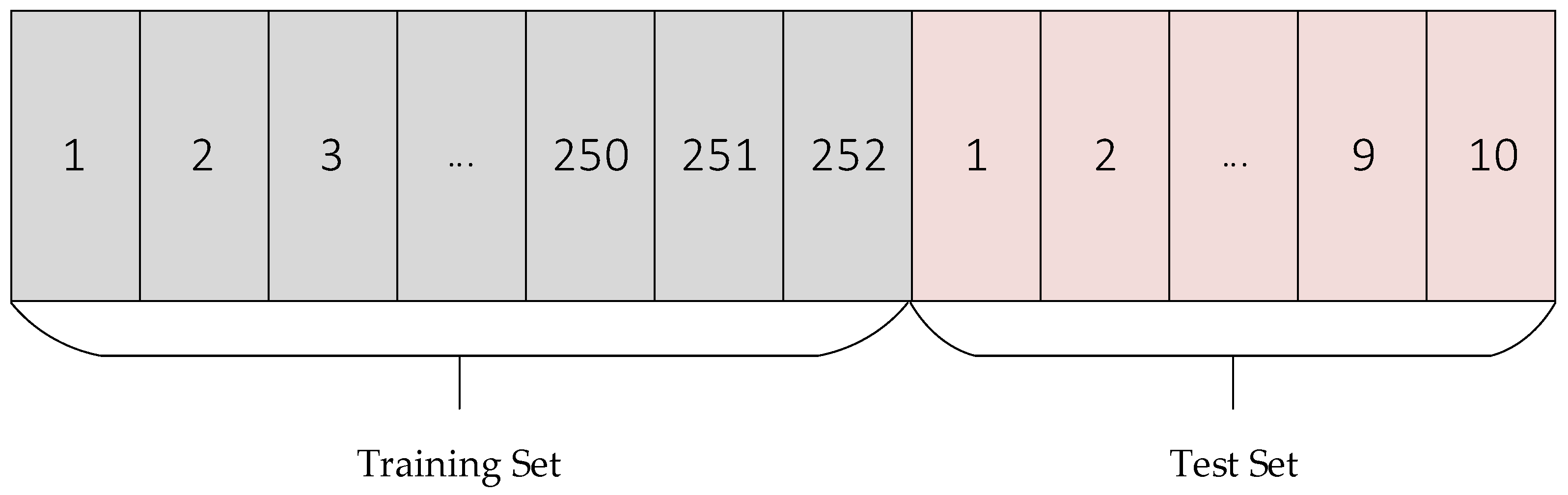
Considering a long memory of fractional Brownian motion, this paper selected as a market cycle [40] (252 day,) as the observation data set; the prediction is the next ten trading days of the index trend, that is, 1 July 2019–15 July 2019, based on the past year’s trading day data predicted from the same data after that. As shown in Figure 2, the experimental data uses a sliding window (windows = 252) to move backward and forward by 10 trading day lengths each time, so as to obtain the complete set of predicted data.

Here, the prediction performance of the GBM, GFBM, MFBM, and IFPSO-MFBM models proposed in this paper are compared for stock price trends. The forecasting results of the four models are analyzed.

4.3.1. SSE Index Data Prediction Analysis

This experiment uses the Chinese A-share SSE index dataset to validate the model prediction effect. The main data is the daily closing price of the SSE index from 1 July 2019–1 July 2022.

• Parameter solving and optimization

The parameters in the MFBM model are solved and optimized according to the steps in Section 3.

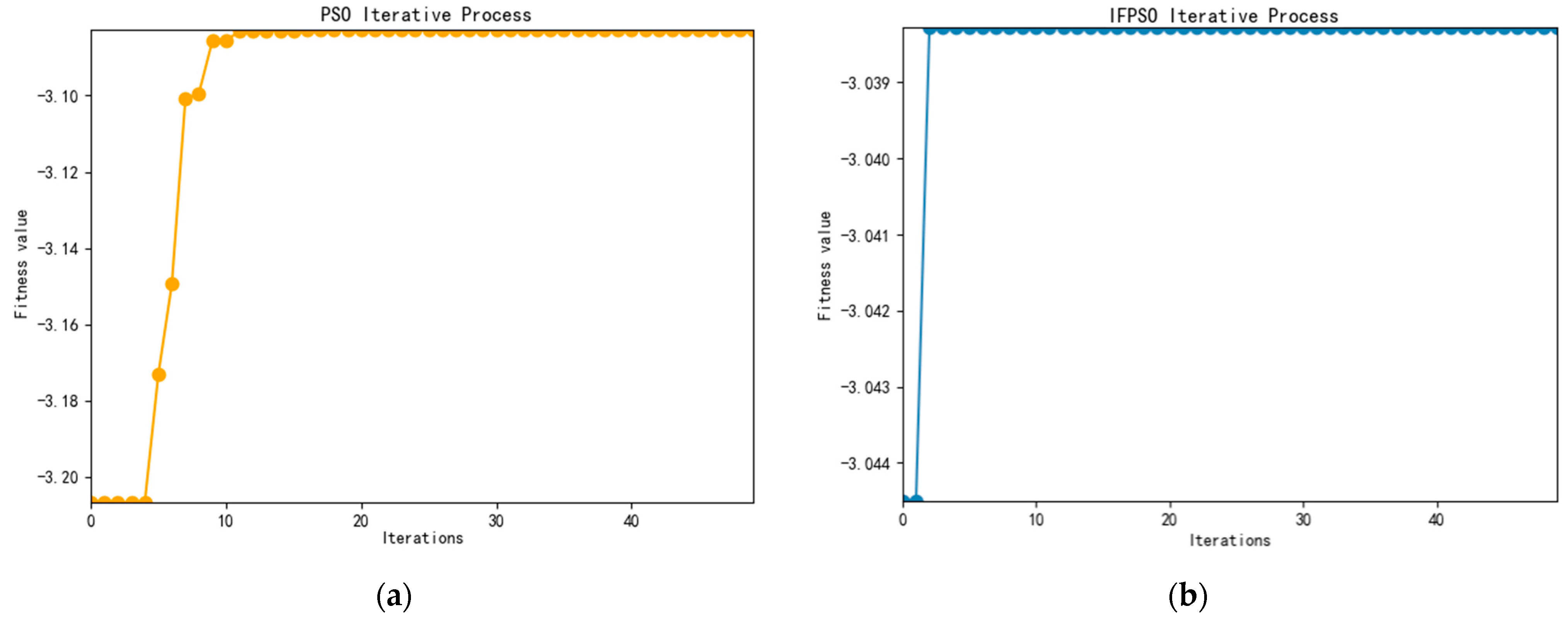
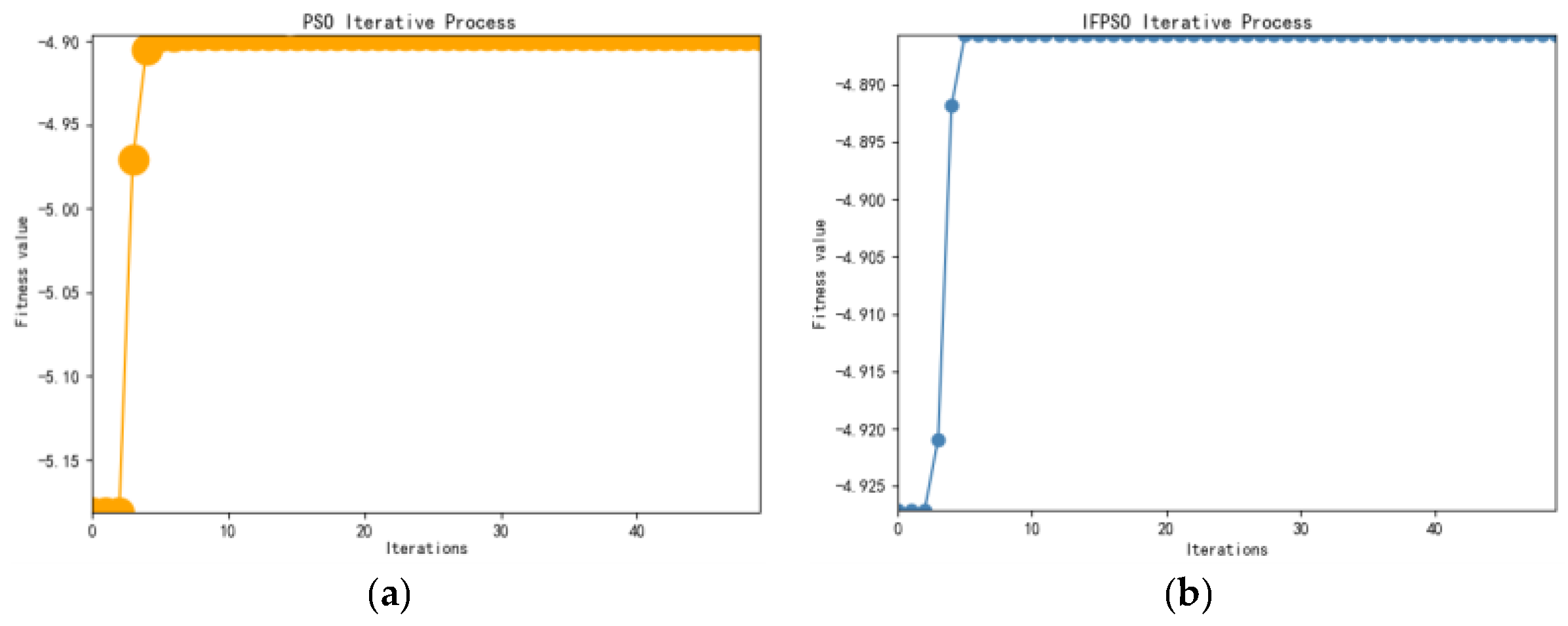
From Figure 3, it can be seen that improved fractional-order particle swarm algorithm (IFPSO) outperforms the particle swarm algorithm (PSO) in terms of both convergence speed and merit-seeking effect. The results are shown in

Table 2. MFBM model parameters and optimization results for the SSE index.

Index Set	Parameters	R/S	MLE	IFPSO
SSE	$\mathsf{\mu }$	-	0.0521	0.1209
	$\mathsf{\sigma }$	-	0.1739	0.1221
	$\mathsf{\rho }$	-	-	0.7893
	$\mathrm{H}$	0.5214	-	0.5334

.

Based on the SSE index data, the mean Hurst value of 0.5214 is first obtained by R/S analysis. Then, we obtain $\stackrel{`}{\mathsf{\mu } }$= 0.0521 and $\stackrel{`}{\mathsf{\sigma } }$= 0.1739 by the MLE method. Since the value by the MLE method is not optimal, it is further optimized by the IFPSO algorithm in this paper to obtain $\mathsf{\mu }$= 0.1209, $\mathsf{\sigma }$= 0.1221, and $\mathsf{\rho }$= 0.789. To reduce the influence of the initial value, the Hurst value is also optimized using the IFPSO, and H = 0.5334 is finally obtained. The change in optimization is evident in the data. The final optimization effect is judged by the magnitude of MAPE, SMAPE, and R2.

The seed is the random seed number of the random model. The experiment takes the best seed value in the seed (1~200).

2.

Comparison of Simulation Results

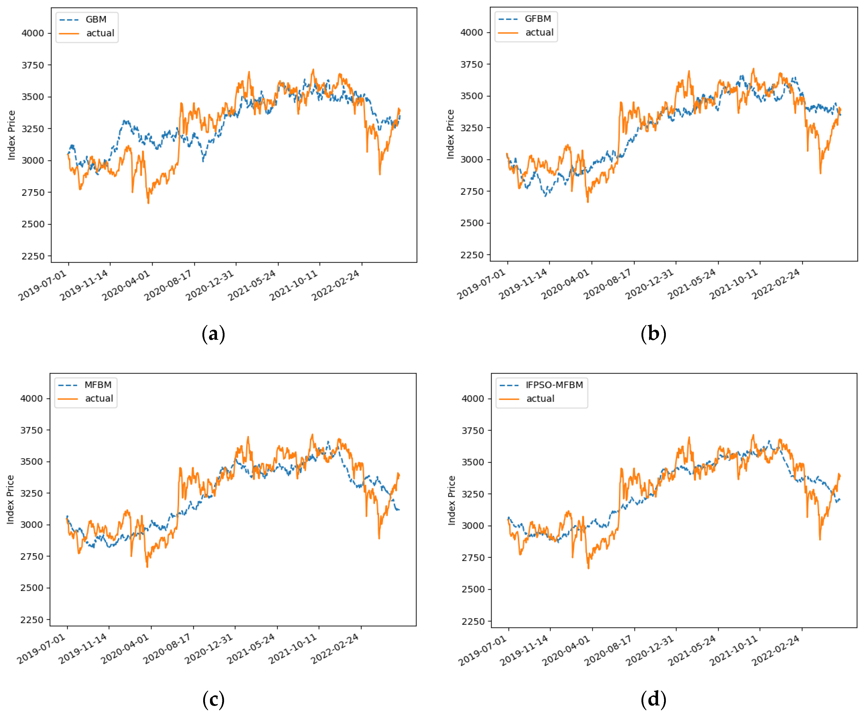
The parameters of the four models (GBM, GFBM, MFBM, and IFPSO-MFBM) are set as in

Table 3. Parameters of the SSE in the four models.

Index Set	Model	Seed	$\mathsf{\mu }$	$\mathsf{\sigma }$	$\mathsf{\rho }$	Hurst
SSE	$\mathrm{GBM}$	87	0.0521	0.1739	-	-
	$\mathrm{GFBM}$	136	0.0521	0.1739	-	0.5214
	$\mathrm{MFBM}$	143	0.0521	0.1739	0.5	0.5214
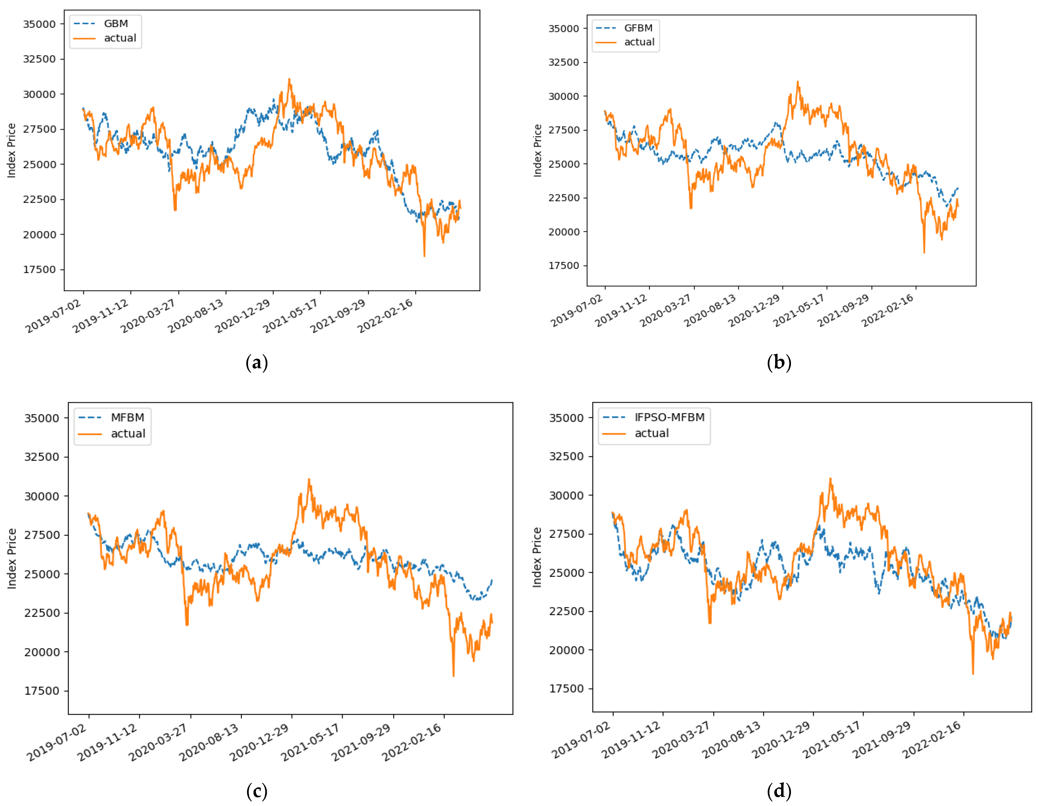
	$\mathrm{IFPSO}-\mathrm{MFBM}$	143	0.1209	0.1221	0.7893	0.5334

. The experimental comparison images are as follows:

Figure 4a shows the result of the predictive simulation of the SSE in the GBM. The main parameters of the model are Seed = 87, u = 0.0521, and $\mathsf{\sigma }$= 0.1739. Figure 4b is the result of the predictive simulation of the SSE in the FBM model. The main parameters have that Seed = 136, u = 0.0521, $\mathsf{\sigma }$= 0.1739, and H = 0.5214. Figure 4c shows the result of the predictive simulation of the SSE in MFBM model, with Seed = 143, u = 0.0521, $\mathsf{\sigma }$= 0.1739, $\mathsf{\rho }$= 0.5, and H = 0.5214. Figure 4d shows the predictive simulation result of the SSE index in the optimized IFPSO-MFBM model. The main parameters are Seed = 143, u = 0.1209, $\mathsf{\sigma }$= 0.1221, $\mathsf{\rho }$= 0.7893, and H = 0.5334. The specific error magnitudes can be shown in

Table 4. Comparative error analysis of SSE index under four models.

Index Set	Model	MAPE%	SMAPE%	R2
SSE	GBM	4.3782	4.2857	0.6089
	GFBM	3.6379	3.6439	0.7163
	MFBM	4.3878	4.4227	0.6247
	IFPSO-MFBM	3.3442	3.3262	0.7019

.

As can be seen, the MFBM model has the largest error in prediction, with a MAPE of 4.3878%. The optimized IFPSO-MFBM has the smallest error, with a MAPE of 3.3342%. The IFPSO-MFBM model has a reduced MAPE of 1.0436% compared to the MFBM model. In addition, the forecasting errors of the SSE index in all four models are less than 10%. It can be proven that all four models achieve high precision forecasting results.

Based on the forecast results, considering an incremental increase of more than 2% per 10 trading days and a forecast error of less than 1% (i.e., the trend is the same and the error is less than 1%), the returns obtained are shown in

Table 5. Comparative analysis of SSE index returns under four models.

Index Set	Model	Returns (1 July 2019–1 July 2022)
SSE	GBM	0.1714
	GFBM	0.1441
	MFBM	0.1545
	IFPSO-MFBM	0.2815

.

The GBM model return of 17.14%, the GFBM model return of 14.41%, the MBM model return of 15.45% and the IFPSO-MFBM model return of 28.15% can be seen. All four models returned greater than 10%, and the MFBM model had the best return

4.3.2. Hang Seng Index Data Prediction Analysis

This experiment uses the Hong Kong Hang Seng index dataset to validate the model prediction effect. The main data is the daily closing price of the Hang Seng index from 1 July 2019–1 July 2022.

• Parameter solving and optimization

The parameters in the MFBM model are solved and optimized according to the steps in Section 3.

From Figure 5, it can be seen that IFPSO outperforms the PSO algorithm in terms of the merit-seeking effect. The results are shown in the table below.

As can be seen in

Table 6. MFBM model parameters and optimization results for the Hang Seng index.

Index Set	Parameters	R/S	MLE	IFPSO
Hang Seng	$\mathsf{\mu }$	-	−0.0677	0.2631
	$\mathsf{\sigma }$	-	0.2318	0.5820
	$\mathsf{\rho }$	-	-	0.7496
	$\mathrm{H}$	0.5651	-	0.6160

, the mean Hurst value of 0.5651 is first obtained by R/S analysis. Then, we obtain $\stackrel{`}{\mathsf{\mu } }$= −0.0677,$\stackrel{`}{ \mathsf{\sigma } }$= 0.2318 by the MLE method. This is further optimized by the IFPSO algorithm in this paper to obtain $\mathsf{\mu }$ = 0.2631, $\mathsf{\sigma }$= 0.5820, and $\mathsf{\rho }$= 0.7496. The Hurst is also optimized using IFPSO and Hurst = 0.6160 is finally obtained. The change in optimization is evident in the data. The final optimization effect is judged by the magnitude of MAPE, SMAPE, and R2.

The seed is the random seed number setting of the random model, this experiment takes the best seed value in the seed (1~200).

2.

Comparison of Simulation Results

The parameters of the four models (GBM, GFBM, MFBM, and IFPSO-MFBM) are set as in

Table 7. Parameters of the Hang Seng in the four models.

Index Set	Model	Seed	$\mathsf{\mu }$	$\mathsf{\sigma }$	$\mathsf{\rho }$	Hurst
Hang Seng	$\mathrm{GBM}$	107	−0.0677	0.2318	-	-
	$\mathrm{GFBM}$	121	−0.0677	0.2318	-	0.5651
	$\mathrm{MFBM}$	89	−0.0677	0.2318	0.5	0.5651
	$\mathrm{IFPSO}-\mathrm{MFBM}$	89	0.2631	0.5820	0.7496	0.6160

; the experimental comparison images are as follows.

Figure 6a shows a plot of the results of the predictive simulation of the Hang Seng in the GBM. Figure 6b shows a plot of the results of the predictive simulation of the Hang Seng in the FBM model. Figure 6c shows a plot of the results of the predictive simulation of the Hang Seng in the MFBM model. Figure 6d shows a plot of the predictive simulation results of the Hang Seng index in the IFPSO-MFBM model. For the specific error magnitudes, see the table below.

As can be seen from

Table 8. Comparative error analysis of Hang Seng index under four models.

Index Set	Model	MAPE%	SMAPE%	R2
Hang Seng	GBM	5.4472	5.3733	0.4893
	GFBM	6.5526	6.5584	0.2990
	MFBM	6.2164	6.1092	0.3836
	IFPSO-MFBM	4.8857	4.9752	0.5348

, the GFBM model has the largest error in prediction, with a MAPE of 6.5526%. The IFPSO-MFBM has the smallest error, with a MAPE of 4.8857%. The IFPSO-MFBM model has a reduced MAPE of 1.3307% compared to the MFBM model. The IFPSO-MFBM after parameter optimization has been improved to a certain extent. In addition, the forecasting error of the Hang Seng index in all four models are less than 10%. This proves that all four models achieve high precision forecasting results and have a highly accurate forecasting effect.

Based on the forecast results, the returns obtained are shown in

Table 9. Comparative analysis of Hang Seng index returns under four models.

Index Set	Model	Returns (1 July 2019–1 July 2022)
Hang Seng	GBM	0.1474
	GFBM	0.1168
	MFBM	0.1173
	IFPSO-MFBM	0.2307

.

The GBM model return of 14.74%, GFBM model return of 11.68%, MBM model return of 11.73%, and the IFPSO-MFBM model return of 23.07% can be seen. All four models returned greater than 10%, and the MFBM model had the best return

4.3.3. Dow Jones Index Data Prediction Analysis

This experiment uses the US Dow Jones index dataset to validate the model prediction effect; the main data is the daily closing price of the Dow Jones index from 1 July 2019–1 July 2022.

• Parameter solving and optimization

The parameters in the MFBM model were solved and optimized according to the parameter solving and optimization process in Part 3.

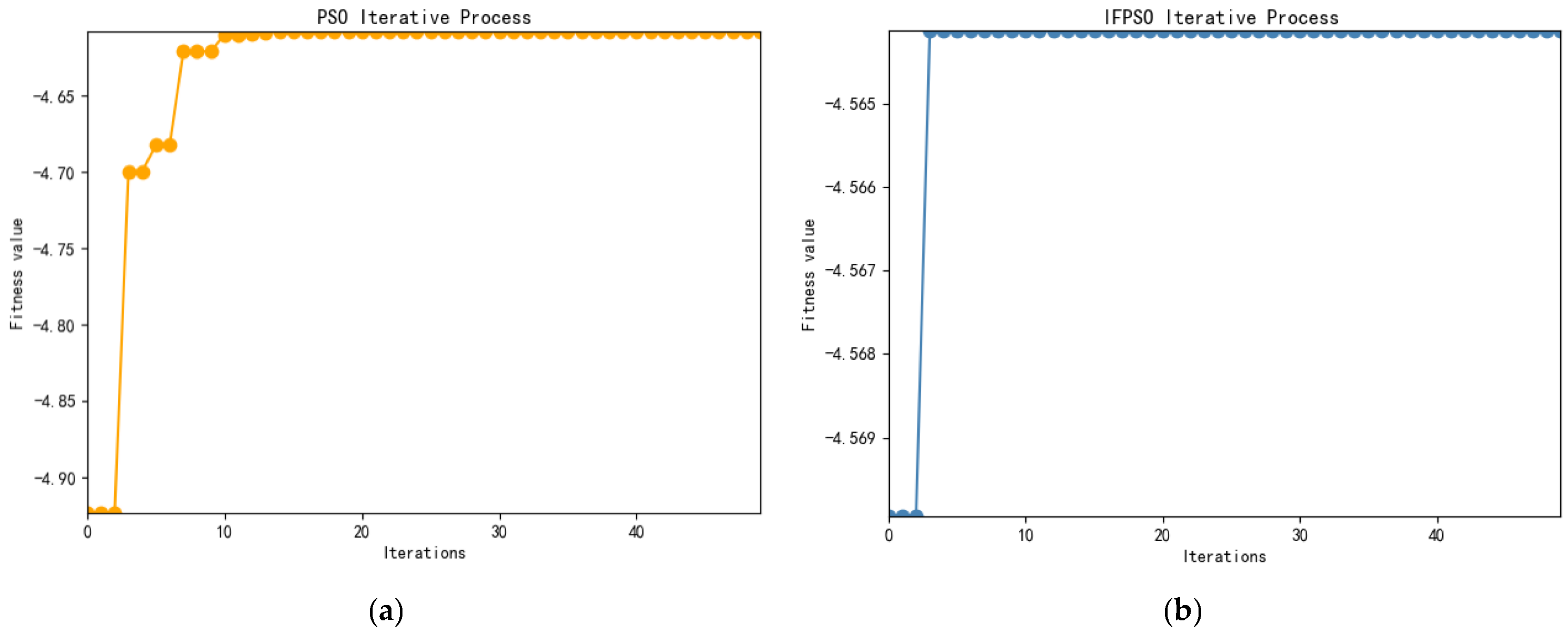
From Figure 7, it can be seen that IFPSO outperforms the PSO algorithm in terms of both convergence speed and merit-seeking effect. The results are shown in the table below.

As can be seen in

Table 10. MFBM model parameters and optimization results for the Dow Jones index.

Index Set	Parameters	R/S	MLE	IFPSO
Dow Jones	$\mathsf{\mu }$	-	0.0804	0.0127
	$\mathsf{\sigma }$	-	0.2436	0.2790
	$\mathsf{\rho }$	-	-	0.3983
	$\mathrm{H}$	0.5939	-	0.5480

, the Hurst value of 0.5939 is first obtained by R/S analysis; then, $\stackrel{`}{\mathsf{\mu }}$= 0.0804 and $\stackrel{`}{\mathsf{\sigma } }$= 0.2436 were obtained by the MLE method. Since the value obtained by the MLE method is not optimal. It is further optimized by the IFPSO algorithm in this paper to obtain $\mathsf{\mu }$ = 0.0127, $\mathsf{\sigma }$= 0.2790, and $\mathsf{\rho }$= 0.3983. To reduce the influence of the initial value, the Hurst is also optimized using IFPSO, and Hurst = 0.5480 is finally obtained. The change in optimization is evident in the data and the final optimization effect is judged by the magnitude of MAPE and SMAPE.

The seed is the random seed number setting of the random model, this experiment takes the best seed value in the seed (1~200).

2.

Comparison of Simulation Results

The parameters of the four models (GBM, GFBM, MFBM, and IFPSO-MFBM) are set as in

Table 11. Parameters of the Dow Jones in the four models.

Index Set	Model	Seed	$\mathsf{\mu }$	$\mathsf{\sigma }$	$\mathsf{\rho }$	Hurst
Dow Jones	$\mathrm{GBM}$	170	0.0804	0.2436	-	-
	$\mathrm{GFBM}$	188	0.0804	0.2436	-	0.5939
	$\mathrm{MFBM}$	52	0.0804	0.2436	0.5	0.5939
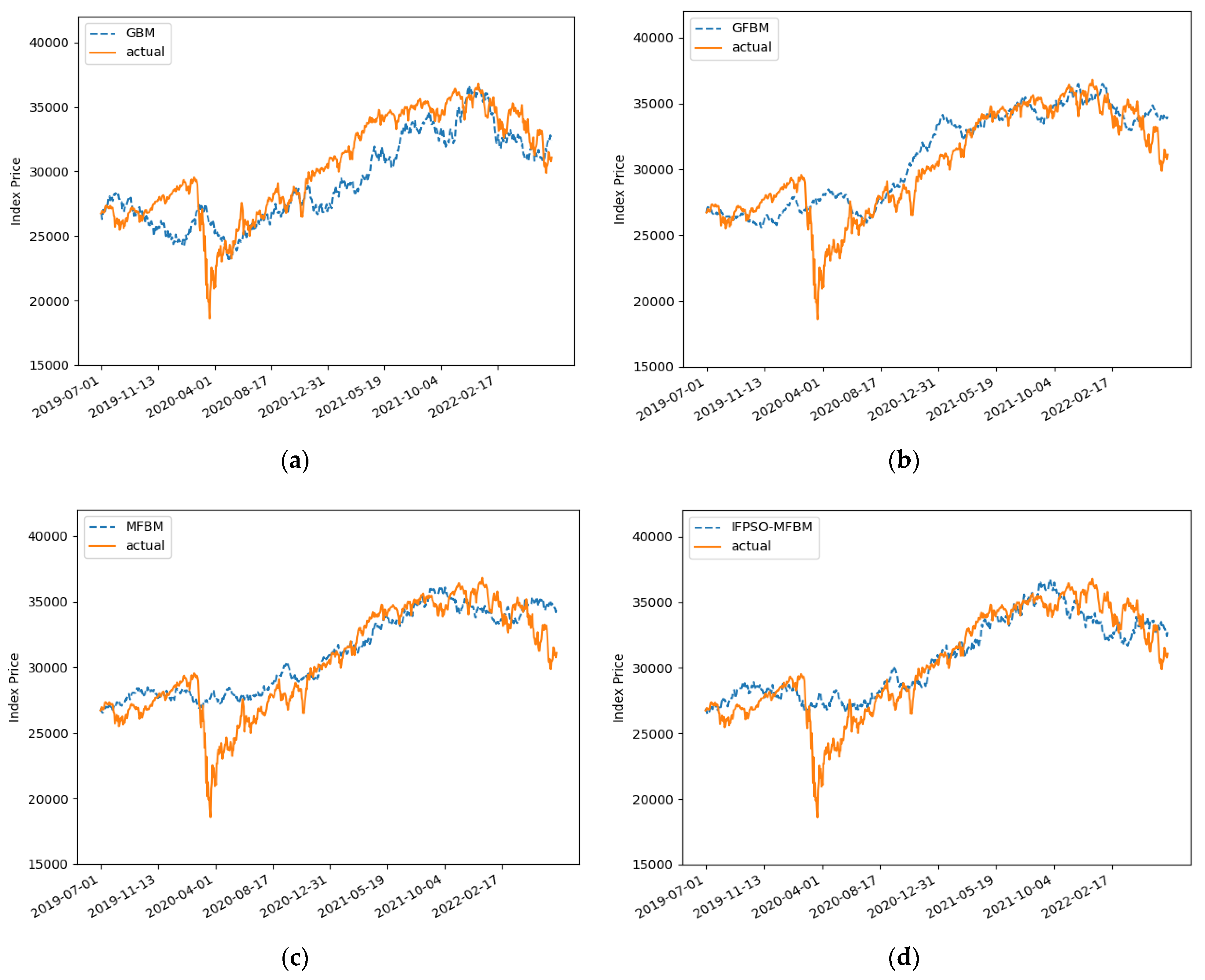
	$\mathrm{IFPSO}-\mathrm{MFBM}$	52	0.0127	0.2790	0.3983	0.5480

and the experimental comparison images are as follows.

Figure 8a shows the result of the predictive simulation of the Dow Jones in the GBM. Figure 8b shows the result of the predictive simulation of the Dow Jones in the FBM model. Figure 8c shows the result of the predictive simulation of the Dow Jones in the MFBM model. Figure 8d shows the predictive simulation result of the Dow Jones index in the IFPSO-MFBM model. For specific error magnitudes, see the table below.

As can be seen in

Table 12. Comparative error analysis of Dow Jones index under four models.

Index Set	Model	MAPE%	SMAPE%	R2
Dow Jones	GBM	6.0259	6.1553	0.6816
	FBM	4.9502	4.7362	0.7591
	MFBM	5.5135	5.3750	0.7113
	IFPSO-MFBM	4.4196	4.1912	0.7662

, the GBM model has the largest error in prediction, with a MAPE of 6.0259%. The IFPSO-MFBM had the smallest error, with a MAPE of 4.4196%. The IFPSO-MFBM model has a reduced MAPE of 1.0939% compared to the MFBM model. The IFPSO-MFBM after parameter optimization was improved to a certain extent. In addition, the R2 of the Dow Jones index in all four models is larger than 0.6, which proves that all four models have a good forecasting effect.

Based on the forecast results, the returns obtained are shown in

Table 13. Comparative analysis of the Dow Jones index returns under four models.

Index Set	Model	Returns (1 July 2019–1 July 2022)
Dow Jones	GBM	0.1426
	GFBM	0.2158
	MFBM	0.1033
	IFPSO-MFBM	0.3083

.

The GBM model return of 14.26%, GFBM model return of 21.58%, MBM model return of 10.33% and the IFPSO-MFBM model return of 30.83% can be seen. All four models returned greater than 10%, and the MFBM model had the best return

From three experiments, it can be shown that the IFPSO-MFBM has the best result of the four models. The MAPE is reduced by 0.9203% on average and the returns are greater than 20%. The IFPSO-MFBM has a more significant improvement.

5. Conclusions

The efficient market hypothesis and the fractal market hypothesis are combined in this paper to study the stock forecasting problem. Firstly, the shortcomings of geometric and fractional Brownian motion are analyzed and the MFBM model is constructed. Then the fractional-order particle swarm optimization algorithm is improved. Last but not least, the IFPSO-MFBM is proposed to forecast stock price.

For the GBM model, there is a clear error in the price prediction. The graph is normally distributed, but the real share price follows the “spike and thick tail”, which does not match the specific form of the share price. The fractional Brownian motion model has arbitrage and is not a sound mode. The MFBM has memory and eliminates arbitrage, and it enables better forecasting of stock prices. However, its parameters are not optimal.

Most stock price time series have a long memory in nature. The Hurst index is the most commonly characterized method. However, in practical applications, R/S analysis method has some obvious shortcomings for calculating long memory parameters and the obtained Hurst values are not optimal. Therefore, the Hurst values are further optimized by IFPSO. Other coefficients are optimized by the improved fractional-order particle swarm optimization algorithm. The final MFBM model with optimal parameters is obtained, which is the IFPSO-MFBM model. Through experimental analyses, it can be found that the IFPSO-MFBM model is superior to GBM, FBM, and MFBM models in stock price prediction.