Abstract
The growing impact of human activities on the environment has increased their influence on the planet’s natural cycles, especially in relation to the hydrological cycle of watersheds. The fundamental processes for its water and energy balance have been affected, which influences water availability and surface streamflow. This study sought to evaluate the anthropogenic impacts on the hydrological cycle of the São Francisco River Basin (SFRB), Brazil, between 1985 and 2015. The study area comprised SFRB and 10 sub-basins for general and specific analyses, respectively. Analyzed data consisted of Land Use and Land Cover (LULC), precipitation, streamflow, and temperature. The methodology incorporated: (i) assessment of LULC dynamics; (ii) trend analysis with the Mann–Kendall method and Sen’s Slope; and (iii) decomposition of total streamflow variation via Budyko’s hypothesis and climate elasticity of streamflow. As a result, it was possible to detect an anthropic modification of SFRB, which is the main component of its streamflow variation, in addition to increased streamflow sensitivity to climate variations. In addition, the divergent behavior in the trends of hydrological variables suggests a change in the streamflow response to precipitation. Therefore, the results allowed us to identify and quantify the impacts of anthropic modifications on the hydrological cycle of the SFRB.
1. Introduction
The rapid growth of the world population has led to fast growth in the demand for water, energy, and food, among other basic necessities for the functioning of modern society [1,2]. In this scenario, the anthropic alteration of the Land Use and Land Cover (LULC) and, consequently, the consumptive water demands for these uses may have intensified over the last few decades in order to meet those necessities.
In the global context of increasing anthropic modification of the environment, water availability and surface streamflow have become dependent on both natural and anthropic factors. The impact of the latter on the global hydrological cycle can be direct or indirect. Among the indirect ones, one can cite the climate changes associated with the emission of greenhouse gases. The direct ones, in turn, comprise the growth of consumptive water demands, modification in the natural conditions of LULC, and streamflow regularization, among others [3,4,5].
In Brazil, as pointed out by [6], between 1985 and 2017, about 38% of Brazilian territory was modified by agriculture and livestock activities and, less expressively, by the expansion of the urban infrastructure, changing the forest, and natural non-forest formations in all six Brazilian biomes. In parallel with this, Ref. [7] pointed out that there was a reduction of 15.7% in the Brazilian water surface between 1991 and 2020, equivalent to 3.1 million hectares, being observed decreasing trends in most of its hydrographic regions. This behavior suggests a reduction in Brazilian water availability, which may affect multiple users of this resource.
In a watershed, anthropic alterations can affect its hydrological cycle. These modifications influence the precipitation-flow relationship, altering the generation of superficial streamflow and the basin’s response to extreme events, such as droughts or floods, intensifying, or relieving them, depending on the anthropic changes carried out [8,9]. Furthermore, these modifications can alter evapotranspiration patterns, interfering with the energy and water balance of the basin [10,11].
The São Francisco River has singular importance for Brazil and mainly for the arid region of the Brazilian Northeast (BNE). In its watershed, the São Francisco River Basin (SFRB), multiple consumptive and non-consumptive uses are met, e.g., irrigation, industrial use, hydropower generation, fishing, sailing, among others [12].
For 30 years (1991–2020), the SFRB presented a reduction of 15% in its water surface [7]. Insufficient water availability in this basin awakens large concerns among water managers because it generates impacts on the multiple social and economic sectors that depend, directly or indirectly, on SFRB water resources.
The increase in water demands for the multiple users installed at SFRB has imposed conflicting situations among them. These conflicts were intensified by prolonged droughts that affected the BNE, such as the 2012–2018 drought, which contributed significantly to the reduction of water availability in this basin [13,14,15].
The influence of climatic factors on the streamflow observed in SFRB, such as the low-frequency oscillations of Sea Surface Temperature (SST) in the Pacific and Atlantic Oceans, was found in several studies [16,17,18].
Regarding anthropic factors, studies that evaluate the impacts of these factors on the behavior of the streamflow in SFRB as a central theme are still scarce, causing this problem to usually be treated in a secondary way. However, recent studies, such as those of [19,20], have brought these impacts to the center of discussion.
Given the possible impacts of anthropic modifications in a watershed, monitoring and understanding these impacts are indispensable for the sustainable management and exploitation of natural resources [21]. In the SFRB, where conflicts in water allocation are already evident, reflecting a water scarcity situation, the anthropic modification and its impacts must draw special attention, given the importance of this basin for different Brazilian social and economic sectors.
Therefore, this paper aims to analyze the impacts of anthropic changes on the surface streamflow of the SFRB between 1985 and 2015, establishing relationships between the observed LULC dynamics and the behavior of the hydrological variables analyzed. The proposed discussions in this paper highlight the influence of anthropic modifications in the hydrological cycle of a watershed, evidencing the need for integrated planning of water resources that considers the dynamics of LULC.
2. Materials and Methods
2.1. Study Area
The study area comprised the SFRB (Figure 1). The São Francisco River has strategic importance for Brazil because it meets multiple consumptive and non-consumptive water demands, with the benefits of these uses transcending, in some cases, the spatial limits of the basin, e.g., the hydropower generation in the Brazilian National Interconnected System (NIS) and water transposition between basins.
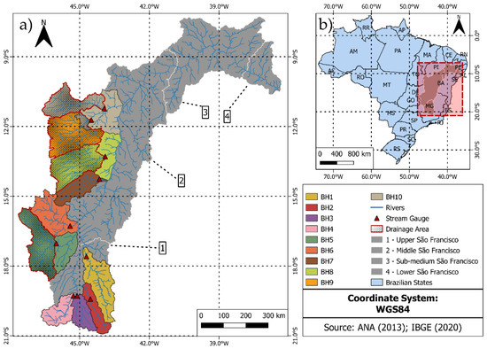
Figure 1.
(a) Study area, the SFRB, and its 10 evaluated sub-basins, as well as the stream gauges that represented the outlets of these last, in (b) an overview of the SFRB throughout the Brazilian States.
The SFRB has a drainage area of 639,129 km2 and an extension of 2863 km. Along with its extension, it connects two Brazilian macroregions (southeast to northeast Brazil) flowing into the Atlantic Ocean. Throughout the drainage area, climate, and environmental diversity can be observed. All this diversity gives to São Francisco River its popular name: The River of National Integration.
According to [12], the SFRB can be divided into four water resources management and planning units: Upper São Francisco (USF), Middle São Francisco (MSF), Sub-Medium São Francisco (SSF), and Lower São Francisco (LSF), as highlighted in Figure 1. There are approximately 18 million inhabitants in these units, with the highest population density in the USF, which encompasses part of the Brazilian metropolitan region of Belo Horizonte in Minas Gerais state.
SFRB serves multiple consumptive and non-consumptive uses, such as hydropower generation, irrigation, human supply, and navigation. The water availability, based on Q95 of the flows in the reservoirs’ lakes and their downstream, is 821 m3/s and an average annual flow of 2057 m3/s [22].
Hydroelectric generation in the SFRH has an important role in the Brazilian energy supply, with installed hydroelectric power that corresponds to about 11% of total installed hydroelectric power in all Brazilian NIS. Among the main hydroelectric plants in this basin, the following stand out: Sobradinho, Três Marias, and Itaparica [23,24,25].
As shown in Figure 1, in addition to the SFRB as the study area, 10 SFRB sub-basins were also delimited to perform more comprehensive analyses of the impact of anthropic changes in its hydrological cycle. The stream gauges highlighted in Figure 1 represent the outlets of the sub-basins. In some situations where it was far from a real outlet, the drainage area of this station was delimited, using it to represent the evaluated sub-basin.
These sub-basins were extracted from a division of SFRB into 34 sub-basins presented in the National Water Resources Plan for the São Francisco River Basin (PRHSF, from Portuguese) [26].
The choice of 10 sub-basins for a more thorough analysis of the impacts of anthropic alteration in the SFRB was due to three reasons: (i) As [27] say, on a regional scale, the climate variability and the anthropic factors interact with each other, combining their effects; in a basin or sub-basin scale, these two modifying agents of the hydrological cycle can be considered independent; (ii) The chosen sub-basins do not have flow regulation structures, because, in basins with those structures, mainly through accumulation reservoirs, the signals of anthropic alteration can be smoothed or even camouflaged by the flow regularization and (iii) they are headboard sub-basins, avoiding that the alterations in upstream sub-basins may interfere with the analyses of the evaluated area.
2.2. Used Data
The data used included both LULC and hydrological data. The time series of these data comprised the period from 1985 to 2015. The lower limit of this period was delimited by LULC data, which began in 1985. The upper limit, in turn, was delimited by hydrologic data because, from 2015, many stations were discarded in the failure analysis.
2.2.1. Hydrological Data
The hydrological data refer to precipitation, streamflow, and temperature. The precipitation and streamflow data were obtained from the HIDROWEB database of the Brazilian National Water Agency, and the temperature data were obtained from the Climate Research Unit (CRU) database. Furthermore, precipitation data from the Global Precipitation Climatology Centre (GPCC) were also used to correct eventual inconsistencies or failures in the monthly rainfall series.
The precipitation series obtained for the SFRB were filtered based on a daily failure criterion. This criterion consisted of the approval of the stations that presented more than 300 days of measurements in each year of the adopted period (1985–2015). Despite this criterion allowing up to two months (60 days) without measurement in each year, all the approved stations showed at most 1 month absent per year throughout their time series.
The approved daily rainfall series gave rise to the monthly precipitation series. In situations where absence or inconsistency was observed in a given month of the last series, data from the GPCC grid point closest to this station were used to fill the monthly gap or replace the inconsistency.
GPCC is a research center operated by the National Meteorological Service of Germany, the German contribution to the World Climate Research Programme (WCRP). Its main function is the global analysis of daily and monthly precipitation over the Earth’s surface, based on in situ observed precipitation data. The final product of this analysis is a grid of precipitation over the Earth’s surface with resolutions of 0.25°, 0.5°, 1.0°, and 2.5° for latitude and longitude [28]. In this study, the GPCC’s grid of monthly precipitation with a resolution of 1° was utilized.
The streamflow series, in turn, were also filtered by the same failure criterion used to select the precipitation series suitable for consideration; however, in case of eventual inconsistencies or monthly failures, the stream gauge was discarded.
The temperature data were obtained from CRU’s database. As pointed out by [29], the CRU’s database provides a high-resolution grid (0.5° × 0.5°) of in situ observation for 10 variables (observed and derived) since 1901. In the present work, the derived variables of maximum and minimum temperature at 2 m from the surface were used. For each grid point contained in the SFRB, the potential evapotranspiration (PET) was determined with the Hargreaves–Samani method.
In the sub-basins analysis, the Thiessen method was used to determine both the averages of precipitation and PET in each of the 10 sub-basins highlighted in Figure 1. In a more general analysis of the SFRB, the stations and grid points mentioned above were used punctually.
2.2.2. Land Use and Land Cover Data
The LULC classification for the SFRB was obtained from a historical series of annual maps of the Brazilian LULC from Collection 6 (Col. 6) of the Mapbiomas project. This project is composed of a multidisciplinary team that has generated a historical series of annual maps with the Brazilian Land Use classification, comprising the period from 1985 to 2020 [30]. These maps and their descriptions are provided free of charge (https://mapbiomas.org/ (accessed on 8 January 2022)) in raster format with a latitudinal and longitudinal resolution of 30 m.
The classification methodology used to produce these maps follows a hierarchical system with 4 classification levels. It is possible to establish a correlation between the classification system adopted by Mapbiomas and those adopted by the Food and Agriculture Organization (FAO) and by the Brazilian Institute of Geography and Statistics (IBGE, from Portuguese Instituto Brasileiro de Geografia e Estatística). Furthermore, the Mapbiomas’ classification classes are organized into three groups, referring to the type of LULC: (i) anthropic, (ii) natural, and (iii) mosaic. The latter includes classification classes in which it was not possible to distinguish between anthropic and natural [6,30]. Table 1 shows the hierarchical classification system adopted by the Mapbiomas project in Collection 6, highlighting the different levels of this system and the LULC type.

Table 1.
LULC classes adopted by Mapbiomas in Col. 6.
The global accuracy of Col. 6 in its LULC classification is 90.8% for the level 1 classes, 87.4% for the level 2 classes, and 87.4% for the level 3 classes, not being made available information about the accuracy of level 4 classes until the moment [30].
Two approaches were performed with the LULC data in raster format made available by Mapbiomas: (i) an analysis of the percentage area evolution of each class of LULC considered between the years 1985 and 2020 and (ii) spatial analysis of the LULC dynamics in the same period.
In the first analysis, the use of percentage area was due to the discrepancy in the order of magnitude of the absolute values of the areas between some classes. In both analyses, only the level 1 classes of the Mapbiomas’ classification system (Table 1) were considered, with punctual differences. In the first analysis, the planted forest class (level 2) was separated from the farming class (level 1), and the urban infrastructure class (level 2) was also separated from the class non-vegetated area (level 1), being evaluated separately in both cases. In the second analysis, the forest class (level 1) was dismembered in its level 2 classes: forest formation, savanna formation, mangrove, and wooded restinga, and the planted forest class (level 2) was separated from the farming class (level 1) and presented separately.
2.3. Potential Evapotranspiration Estimation
The Hargreaves–Samani method [31] was used to estimate PET. This hydrological component can be understood as the evaporative demand of the environment based on specific climate conditions, often estimated considering the hypothetical situation of a large cultivated area with grass. Several methods have been developed to estimate it based on climate data, such as the Hargreaves–Samani equation [32].
Still, according to [32], the Hargreaves–Samani equation can be used to determine the PET based on maximum and minimum air temperatures, as shown in Equation (1):
where: PET is given in , are the average, maximum and minimum temperature in degrees Celsius; is the average extraterrestrial solar radiation . The can be estimated based on latitude and month of year, according to [31].
2.4. Trend Analysis
In the trend analysis, the monthly time series of precipitation, streamflow, and PET gave rise to annual time series, such as annual accumulated precipitation, annual average streamflow, annual minimum monthly streamflow, annual maximum monthly flow, and annual accumulated PET. This analysis included the application of the non-parametric Mann–Kendall test and Sen’s slope determination in those annual series. The significance level adopted in each of these methods was 0.05 .
Trend analysis was performed on all selected stations and all CRU grid points used for PET estimation. All the annual time series mentioned above were standardized with a z-score, returning a dataset with a mean equal to zero and a standard deviation equal to one. This standardization was performed to allow for a comparison between the intensity of the detected trends in the evaluated time series.
Additionally, trend analysis was performed in the 10 considered sub-basins using the time series of annual accumulated precipitation, annual accumulated evapotranspiration, and annual average streamflow. It is worth noting that the first two series were considered spatially in the sub-basin.
2.4.1. Mann–Kendall Test
The Mann–Kendall test is widely used to check for growth or decline trends in a data time series. The wide use of this method is due to the lack of need for an initial presumption of the statistical distribution of the dataset and the lower sensitivity to outliers [33].
As pointed out by [34], the statistical variable of the Mann–Kendall test for a time series composed of a sample of random variables identically distributed is given by Equation (2):
with: the statistical variable of the Mann–Kendall test, the size of the time series. The sign function expressed in Equation (2) is given by Equation (3):
The determination of S statistic by comparing pairs of values of the time series, assigning the value of this comparison through sign function (Equation (3)), grants the resistance to outliers for the Mann–Kendall test.
According to [35], when , the statistical variable resembles a normal distribution, with variance determined by Equation (4):
where: is the variance of the statistic, is the number of repetitions in an extension of the time series, e.g., a series with two equal values would have one repetition with extension equal to 2 .
With the variance of statistic, the standardized index , which follows a normal distribution with a mean equal to zero and a standard deviation equal to one, can be determined by Equation (5):
As pointed out by [36], the Mann–Kendall test considers that the null hypothesis indicates an absence of a trend. Thus, because it is a two-tailed test, at a significance level , this hypothesis is rejected if . The standardized index is the value that has an exceedance probability equal to half the significance level adopted in a normal distribution. Furthermore, the index makes it possible to differentiate between a growth trend and a decreasing trend .
Still, according to [36], due to the similarity of the statistic to a normal distribution, it is possible to determine the p-value for the sample data with the cumulative probability of a normal distribution. Therefore, can be tested with the p-value: if there is evidence to reject , so there is indicative of a trend in the analyzed time series.
2.4.2. Sen’s Slope
One of the Mann–Kendall test’s shortcomings is the inability to indicate the magnitude of the detected trend. However, methods external to the test can determine this magnitude, such as Sen’s slope estimate method proposed by [37].
As pointed out by [38], Sen’s slope is determined by calculating the slope between all possible pairs of dataset elements, as represented in Equation (6):
where: is the slope of the i-th data pair; are the j-th and k-th dataset values; are the indexes of elements which form the pairs, being always Since the slope is determined by pairs of values, then there will be slopes, with equals to sample size.
The overall slope of the dataset is the median of all slopes calculated for these data pairs. Sen’s slope provides a realistic measure of the time series trend, is not sensitive to outliers, and allows for the absence of data throughout the series [38].
2.5. Analysis of the Anthropic Changes’ Impact on the Surface Runoff—Conceptual Approach
The analysis of the anthropic changes’ impact on the surface runoff of the SFRB via a conceptual approach was applied in the 10 analyzed sub-basins. The conceptual approach included the Budyko equation and its derivations, such as the Fu equation, and the decomposition of streamflow variation via the Budyko curve.
Initially, in order to apply this conceptual approach, it is necessary to transform the streamflow from to through Equation (7), where is the streamflow and the basin area :
The total period of the time series (1985–2015) was divided into three subperiods: P1 (1985–1995), P2 (1996–2005), and P3 (2006–2015). The division into subperiods was necessary for the assignment of a base period (P1)—where it was sought to refer to the more natural conditions that the data allowed exploration—and a modified period—where it represented the modified state of the basin. Therefore, it was possible to evaluate the streamflow alteration of the analyzed sub-basins from a base period.
The choice of subperiods was arbitrary; however, it was sought to divide 31–year time series into intervals of the same size. Moreover, the adopted subperiods’ size made it possible to consider long–term averages, which underpins the conceptual and analytical approach.
2.5.1. Budyko Hypothesis
Evapotranspiration is one of the main components of the hydrological cycle, playing a vital role in its water and energetic balance [39]. In such a manner, Budyko sought to relate it to hydrological variables that were easier to obtain, such as PET and precipitation.
According to [40], the water balance of a basin is a function of several parameters that refer to the surface and underground characteristics of the basin and to climatic factors; however, it is possible to summarize the main contributions to this balance in and in precipitation , with the other factors being little significant. Thus, the water balance can be simplified as expressed in Equation (8):
with: the precipitation , the evapotranspiration , the flow rate and internal basin storage .
For the long-term analyses, the internal basin storage can be considered equal to zero because this variation occurs within the hydrological year, and the long-term analyses, e.g., in decade intervals, are performed using annual averages [20,39,41,42].
The energy balance in the Budyko hypothesis, in turn, can be summarized in two factors: evapotranspiration and sensible heat flow , i.e., the net radiation near the surface is the sum of the latent and sensible heat fluxes, as shown in Equation (9), where is the heat of water vaporization:
Therefore, Budyko’s hypothesis is structured in two limit conditions (Equation (10)): (i) when the aridity index tends to infinity, the tends to total precipitation, i.e., is limited by the available water, and (ii) when the aridity index tends to zero, the decreases in relation to precipitation, being limited by available energy [42]:
Based on Equation (10) and the considerations presented for water and energy balances, [40] proposed that the ratio between the average annual evapotranspiration and average annual precipitation is a function of the ratio between the average annual PET and average annual precipitation, and of the basin characteristics, as shown in Equation (11). It is worth mentioning that PET represents the maximum net radiation near the surface that can be used for water evaporation [20,39,41,42]:
The function needs to be defined for each analyzed basins because it depends on their characteristics and may have different formats according to the analyzed area.
2.5.2. Fu’s Equation
Several equations that relate the ratio with the ratio were developed based on the Budyko hypothesis, such as Fu’s equation [43], which is analytically derived in [44].
In this equation, the ratio is a function of the ratio and of a parameter which refers to the physical characteristics of the basin that affect how the precipitation is transformed into evaporation and surface runoff, e.g., the dynamics of the relation among vegetation type, soil properties, and topography. As pointed out by [44], high values of suggest favorable characteristics to evapotranspiration and vice-versa [39,42]:
Without an estimate of , it is impossible to obtain by the Fu equation. However, in a long-term analysis, real evapotranspiration can be obtained by the water balance of the Budyko hypothesis, making it possible to estimate .
2.5.3. Decomposition of Streamflow Variation via the Budyko Hypothesis
The Budyko-type curve allows the separation of the climatic and anthropic contributions of the total variation in long-term average flow.
In the long-term analyses, it is valid to simplify the variation of the internal storage of the basin in the water balance of the Budyko hypothesis; thus, the streamflow can be expressed as a function of and , as shown in Equation (13):
Taking the Fu equation as an example:
where: is the Fu equation, is the parameter of Fu Equation and are the long-term average of annual streamflow, annual precipitation, annual potential evapotranspiration and annual evapotranspiration, with all variables in .
As pointed out by [39,41], the decomposition of the total variation of streamflow via the Budyko-type curve using the Fu equation consists of the determination of two parameters : (i) for the pre-change period and (ii) for the post-change period. The basic idea of this decomposition, using Figure 2 as a guide, can be summarized in three points:
- The total variation of streamflow (anthropic + climatic contributions) between the pre- and post-change period is equivalent to the difference in streamflow between points C and A, because, among these points, there are changes in the climatic variables: and , and the parameter referring to the physical properties of the basin: ;
- The climatic component of streamflow variation is equivalent to the difference of streamflow between points B and A because, from one point to another, there is only alteration in climate variables: and , and the parameter stays constant;
- The anthropic component of streamflow variation is equivalent to the difference of streamflow between points C and B, since there is alteration only in the parameter referring to the physical properties of the basin , while the climatic variables remain the same.

Figure 2.
Decomposition of total variation in long-term average flow via Budyko-type curve. Source: Adapted from [41].
Figure 2.
Decomposition of total variation in long-term average flow via Budyko-type curve. Source: Adapted from [41].

Through Equation (14), these three points can be expressed mathematically:
where: is the total variation of streamflow; is the streamflow variation resulting from climatic alterations and is the flow variation resulting from the anthropic alterations.
2.6. Analysis of the Impact of Anthropic Changes on Surface Runoff—Analytical Apporach
2.6.1. Streamflow Climate Elasticity
The analytical approach consisted of the application of the concept of the climate elasticity of streamflow. This concept makes it possible to evaluate the streamflow sensibility of climate variations in each period considered. In addition, it can be used to decompose the total flow variation in its anthropic and climate components [39,41,45].
As indicated by [39,42], the climate elasticity of streamflow can be obtained via several methodologies, such as hydrological models, multivariate models, or analytical or empirical equations based on hydrological principles.
Using the Fu Equation, is a function of , i.e., , where is the Fu equation. Thus, the total variation of can be approximated through the first-order expansion of the Taylor series, as shown in Equation (16) [42]:
With the simplification of water balance of the Budyko hypothesis (Equation (8)) for long-term analyses—, the long-term average of annual streamflow can be defined by the difference between long-term averages of precipitation and of evapotranspiration. The same applies to the total variation of these variables:
In this way, by substituting Equation (16) into Equation (17), the total variation of streamflow can be defined as a function of the total variation of precipitation and evapotranspiration:
Assuming that the physical characteristics of the basin do not change over the period taken to determine the long-term averages, then . With this hypothesis, dividing the equation by Q and carrying out the necessary developments, one obtains the following:
With:
Therefore, and are the coefficients of flow elasticity in relation to precipitation and the , respectively. Rewriting Equation (19), one obtains:
The interpretation of this coefficient allows quantification of the sensitivity of the long-term average of streamflow to the precipitation and variations. Exemplifying, a reduction of 1% in the precipitation is equivalent to a reduction of in the streamflow, while an increase of 1% in the results in a decrease of .
2.6.2. Impact Separation via Streamflow Climate Elasticity
As presented by [41,45,46], the concept of the climate elasticity of streamflow allows the separation of the total variation of flow into its climatic and anthropic components. Assuming that these two components are independent, the total variation of the flow can be expressed in terms of the percentage change in relation to a base period, dividing it by the average annual flow of the base period , as shown in Equation (22):
By definition of the climate elasticity of streamflow, Equation (21) represents the variation of the flow resulting from climate alterations . Transforming the differentials of this equation into rates of change between the period of interest and the base period, Equation (22) can be rewritten as follows:
where: is the total variation in streamflow in relation to the base period; is the flow variation resulting from anthropic alterations ; and are, respectively, the rates of variations of average precipitation and average between an evaluated period and the base period ; are, respectively, the averages of flow, precipitation, and of the base period .
Therefore, based on Equation (23), the streamflow variation resulting from anthropic alterations in percentage terms can be determined since the total variation of flow is known due to the observed data, and its climatic component can be obtained with the coefficients of the climatic elasticity of the streamflow and the observed data of precipitation and .
3. Results
3.1. Land Use and Land Cover Dynamics
Figure 3 shows the evolution of the LULC of the SFRB between 1985 and 2015, highlighting the region where the greatest transition from natural to anthropic classes of LULC was observed.
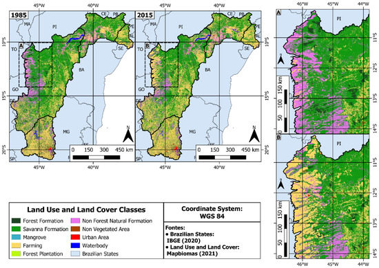
Figure 3.
Spatial evolution of LULC in the SFRB between 1985 and 2015.
Throughout the entire basin, an expansion of agriculture to the detriment of the forest, savanna, and natural non-forest formations can be observed, with the clearest expansion occurring in the west region of the MSF. It also stands out for the expansion of urban infrastructure in the USF. This region (USF) has the highest population density of the SFRB, which is located in the metropolitan region of Belo Horizonte.
Figure 4 shows the evolution of the percentage areas of LULC classes considered between 1985 and 2015 for the ASF, MSF, SSF, and LSF regions. It is emphasized that the classes of forest formation, savanna formation, and mangrove were grouped into the class of natural forest.
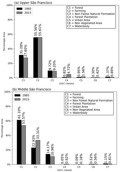
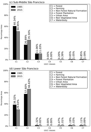
Figure 4.
LULC evolution of each SFRB’s water resources management and planning units: (a) USF, (b) MSF, (c) SSF, and (d) LSF.
Similar behavior was observed in the MSF (Figure 4b), SSF (Figure 4c), and LSF (Figure 4d), where the farming class led the positive variation of the percentage area with +10.38%, +8.61%, and +9.03%, respectively, while the natural forest class led the negative variations with, in the order given, −7.73%, −9.39%, and −8.69%.
In the USF region (Figure 4a), the growth was led by the forest plantation class, whereas the natural forest class led to a decrease, with a variation of −3.68% of its percentage area. The farming class showed little variation; however, it showed great representation in this region, with more than 55% percentage area in both 2015 and 1985. This demonstrates that the USF had already been significantly modified in 1985.
The LULC dynamics of SFRB between 1985 and 2015 evidenced an accelerated modification of the natural conditions of the basin. Taking into account the four management and planning units—USF, MSF, SSF, and LSF—one can classify this dynamic into three groups, considering the initial conditions of LULC and the variation in the adopted period: (i) USF, (ii) LSF, and (iii) MSF and SSF.
The region of the USF showed a LULC dynamic distinct from the other units. In this unit, the largest basin urbanization processes and planted forest area growth were observed; the latter can be justified by the more favorable climatic conditions for this practice in that region.
Although the combined growth of the percentage area of these two classes of LULC did not exceed 5%, it is noteworthy that it occurred mainly to the detriment of natural forest areas. Furthermore, for the initial year, the USF region was already quite modified because 55% of its area was occupied by farming. Therefore, the growth of urban infrastructure and planted forests was added to the pre-1985 changes.
The LSF region presented a predominantly anthropic LULC composition, with the farming area reaching values close to 60% of the basin’s total area, evidencing a rather modified basin prior to 1985. When analyzing the LULC evolution in this region, it is observed that the anthropic alteration prior to 1985 continued until 2015, with the growth of the farming areas reaching 66% of the percentage area. Moreover, the representativeness of urban infrastructure in the total area doubled during the same period. This anthropic expansion took place almost exclusively to the detriment of the natural forest regions.
In the MSF and SSF regions, the LULC dynamic between 1985 and 2015 captured the modification processes of these regions. In 1985, these regions were predominantly occupied by natural forests, at 61.10% and 60.34% of their total areas, respectively. In the evaluated period, a significant reduction in this percentage was observed, reaching a level close to 50% in both regions. These reductions are mainly due to the increase in farming areas, which have augmented their representation in the total area of those regions by around 10%.
3.2. Trend of Hydrological Variables
Figure 5 presents, in a spatialized way, the results of trend analysis performed at all stations of SFRB considered and in all grid points of CRU inside the SFRB, which were used to estimate . Furthermore, it shows the mean and standard deviation used to standardize the time series to enable a comparison between the detected trends in the evaluated hydrological variables.
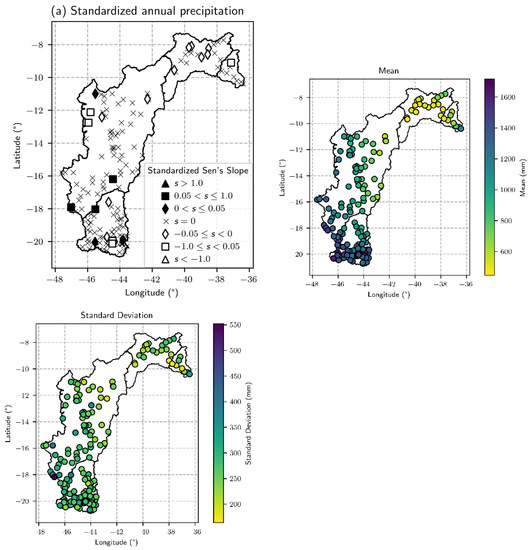
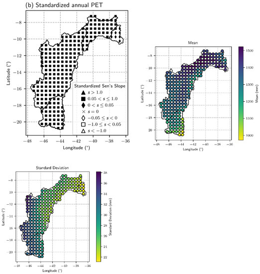
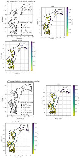
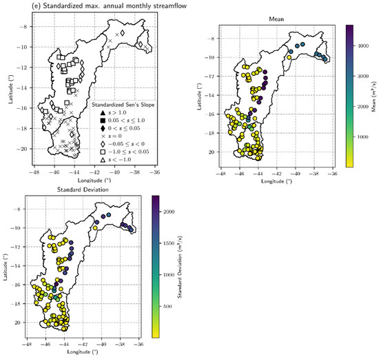
Figure 5.
Standardized Sen’s slope for all SFRB’s stations evaluated and for the CRU’s grid points inside the basin for the following standardized time series: (a) annual precipitation, (b) annual PET, (c) mean annual monthly streamflow (d) minimum annual monthly streamflow, and (e) maximum annual monthly streamflow. Additionally, the mean and standard deviation were used in the standardization process.
The trend analysis results of the annual accumulated precipitation between 1985 and 2015 are presented in Figure 5a. However, some stations presented significant trends, alternating between growth and decline, with the latter types dominating.
The trends in the series of annual from 1985 to 2015 are displayed in Figure 5b. Contrary to what was observed in the annual accumulated precipitation, statistically significant positive trends were found in all CRU’s grid points inside the SFRB. The magnitude of these trends varied in the LSF region, where a reduction in declivity was observed.
Figure 5c–e presents the results of trend analysis for the series of mean, minimum, and maximum monthly flow annual. A similar behavior of decreasing trend was found in all three series, with the concentration of those in the Western region of MSF. It is noteworthy that in the series of annual minimum monthly flows, there was a greater predominance of negative trend stations.
Figure 6 shows the trends in the hydrological variables considered for the evaluated sub-basins. Likewise, the entire SFRB and the time series were standardized to allow a comparison between these variables and between the different sub-basins, since there is a difference in the magnitude of the values in both cases.
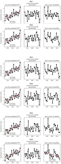
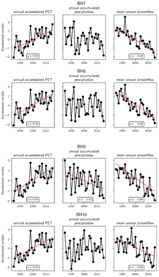
Figure 6.
Trend analysis of annual PET, annual precipitation, and mean annual streamflow for all evaluated sub-basins. Standardized Sen’s slope is represented by .
Two groups of sub-basins can be delimited: (i) the sub-basins with positive trends in and negative trends in mean annual streamflow, and (ii) the sub-basins with positive trends only in . The first group includes the sub-basins located in the USF: BH1, BH2, BH3, and BH4, and a sub-basin that borders this region: BH5. The second group encompasses the sub-basins located in the western region of MSF: BH6, BH7, BH8, and BH10. A particular case is sub-basin BH9, which shows a positive trend in and negative trends in accumulated annual precipitation and mean annual streamflow.
The similarity in the Sen’s slope of the series in all the sub-basins evaluated suggests a similar growth rate in all of them. In the mean annual flow, this slope varied more among the subbasins.
3.3. Impact of Anthropic Changes in Surface Runoff
3.3.1. Conceptual Approach
Figure 7 presents the Budyko-type curves determined with the Fu equation using the three parameters estimated for each adopted period. Moreover, Figure 7 also shows the total variation of the streamflow for the periods P2 and P3 in relation to base period (P1) and its climatic and anthropic components for each case. In all evaluated sub-basins, the total variation of streamflow was negative in the P2 and P3 periods in relation to P1.
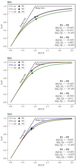
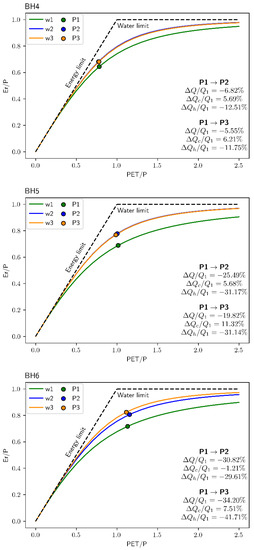
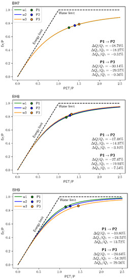
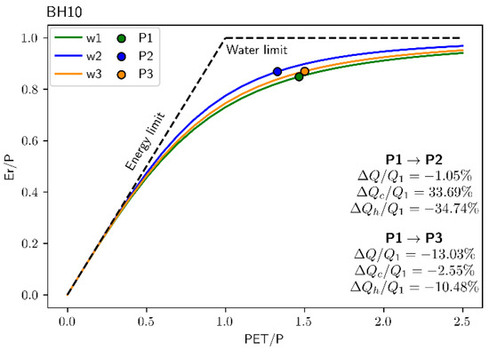
Figure 7.
Budyko-type curve, total streamflow variation, and its climate and anthropic components for periods P2 and P3 in relation to P1 for each evaluated sub-basin. , and are, respectively, the total streamflow variation in relation to the base period and its climatic and anthropic components. and are the parameters of Fu’s Equation (Equation (12)) estimated with the long-term averages of P, ETP and of the periods P1, P2, and P3, respectively.
The evaluation of period P2 in relation to the base period pointed to negative total variations in streamflow in a range from −1.05% (BH10) to −30.82% (BH6). The climatic and anthropic components of this variation changed significantly among the sub-basins.
The climatic component of streamflow variation for P2 in relation to P1 alternated both in the direction of change and in its magnitude. Among the 10 evaluated sub-basins, 6 (BH1, BH2, BH3, BH4, BH5, and BH10) presented positive climate components in a range from +3.23% (BH3) to +33.69% (BH10). The other 4 sub-basins (BH6, BH7, BH8, BH9) showed negative climate components, varying from −1.21% (BH6) to −24.52% (BH9).
Regarding the anthropic component of streamflow variation, the period P2 in relation to P1 exhibited, except for BH9, negative values ranging from −0.52% (BH7) to −34.74% (BH10). In BH9, a positive anthropic component equal to +13.72% was found.
In the evaluation of P3 in relation to the base period, the total variations of flow, in the same way as P2, were negative, varying from −5.55% (BH4) to −34.20% (BH6). Except for BH4 and BH5, the negative total variations in streamflow were higher than in P2.
In relation to the climatic component of streamflow variation in P3, it was observed that the sub-basin with a negative climatic component in P2 had this contribution negatively intensified in P3, except for BH6. Moreover, some sub-basins that presented positive climatic components in P2 had a reduction in magnitude or an inversion in the direction of contribution in P3, such as BH1, BH2, BH3, and BH10, highlighting BH10, which had +33.69% in P2 and −2.55% in P3. Three sub-basins (BH4, BH5, and BH6) presented an increase in positive climate components in relation to P2, highlighting BH6, which had −1.12% in P2 and +7.51% in P3.
The anthropic components in P3, in turn, were negative, except in BH3 and BH9. In BH6 and BH8, the negative anthropic component in P2 was negatively increased in P3. In the other sub-basins, there was a positive variation in this component, reducing the negative values or even changing the direction of contribution, as in BH3. The BH9 showed a positive anthropic contribution in P2 (+13.72%) which intensified in P3 (+29.56%).
3.3.2. Analytical Approach
The analytical approach was carried out using the concept of the climate elasticity of streamflow. Table 2 presents the climate elasticity coefficients in relation to precipitation and PET , determined for the 10 sub-basins evaluated in the three periods considered.
Table 2.
Streamflow climate elasticity coefficients for the evaluated sub-basins. and are, respectively, the coefficients of the climate elasticity of streamflow in relation to precipitation and PET.
Except for BH9, the evolution of these elasticity coefficients over the evaluated periods showed similar behavior, with an increase in its values in periods P2 and P3 in relation to the base period (P1). Comparing the periods P2 and P3, it was observed that in some sub-basin (BH6, BH7, and BH8), the growth behavior remained; however, in the other sub-basins, insignificant variations or even reductions were observed in these coefficients. The exception is the BH9 sub-basins, which presented a decreasing behavior over the evaluated periods.
Table 3 shows the anthropic and climate components of the total streamflow variation for periods P2 and P3 in relation to the base period (P1) obtained with the concept of the climate elasticity of streamflow.
Table 3.
Anthropic and climate components of total streamflow variation for all evaluated sub-basins. , are, respectively, the total streamflow variation and its climatic and anthropic components in relation to the base period.
Evaluating the period P2 in relation to the base period, in the same way as for the decomposition via the Budyko-type curve, it was observed a negative anthropic component of streamflow variation, reaching values close to −40% (BH10). Only in two sub-basins, BH7 and BH9, was this component not predominant in the total variation. The climatic component, in turn, varied in magnitude and direction of the contribution, with the 4 sub-basins with negative values (BH6, BH7, BH8, and BH9) and the others positive ones.
Regarding the streamflow variation of P3 in relation to P1, similar results to those attained via the Budyko-type curve were obtained. The anthropic component was also predominantly negative, arriving at values around −43% (BH6). The two sub-basins with a positive anthropic component in P2 (BH7 and BH9) maintained positive contributions in P3, and the sub-basin BH3 inverted the direction of its contribution in relation to P2.
The contributions of climate components also mimic those obtained in the decomposition via the Budyko-type curve, with sub-basins changing the direction and/or reducing the magnitude of their contributions between periods P2 and P3. The sub-basins with negative climate components in P2, except for BH6, intensified this component in P3. The inversions in the direction of contribution occurred in the sub-basins BH1, BH3, BH6, and BH10, highlighting this last one, which presented +35.98% in P2 and −3.07% in P3. The other sub-basins (BH2, BH4, and BH5) showed variations only in their magnitude between those periods.
4. Discussion
4.1. SFRB LULC Dynamic
The SFRB presented a strong anthropic modification between 1985 and 2015 in some of its regions, while the other regions were already modified in 1985, continuing the anthropic expansion in LULC until 2015. Farming was the predominant use, both in growth in the evaluated period (MSF and SSF) and in representativeness in 1985 (USF and LSF).
This observed behavior between 1985 and 2015 resembles the behavior of the LULC projections carried out by [47] for the SFRB. [47], considering the A2 scenario of the Special Report on Emission Scenarios (SRES) of the Intergovernmental Panel on Climate Change, carried out a LULC projection to 2035. In this projection, there was a doubling of farming areas and a 22% reduction in natural vegetation. To this extent, the social and economic premises of this scenario can be considered active, or partially active in the adopted period from 1985 to 2015. These premises consider, among other points, high population growth and low environmental awareness.
The MSF west region exhibited a large and concentrated expansion of farming areas. This region, highlighted in Figure 3, corresponds to part of an important Brazilian agricultural frontier: the MATOPIBA region.
The MATOPIBA partially covers the Brazilian states of Maranhão, Tocantins, Piauí and Bahia, delimiting an agricultural frontier of high productivity based on large-scale mechanized agriculture for the cultivation of soybean, corn, cassava, and rice. The production of this region increased sixfold between 1995 and 2012, mainly due to large-scale mechanized soy cultivation, doubling Brazilian soy production. In 2013, this region contained 1401 irrigation center pivots, occupying an irrigated area of 138,097 ha. About 90% of these pivots are located in the west of the Brazilian state of Bahia, which coincides with the west of the MSF region [48,49,50].
In addition to the possible direct impacts of the anthropic LULC expansion on the SFRB hydrological cycle, the impacts resulting from the increase in water consumption demands also have an equivalent influence, perhaps greater, on the basin hydrological cycle, e.g., reducing its water availability, as indicated by [3,51].
Ref. [14], evaluating the consumptive demands of the main reservoirs in the SFRB: Três Marias, Sobradinho, and Itaparica, found an increase in consumptive demands for irrigation, human supply, and industry between 1961 and 2017. Irrigation showed the greatest growth, reaching much higher levels than other uses, mainly in Sobradinho (MSF) and Itaparica (SSF).
4.2. Trend of Hydrological Variables
The adopted hydrological variables exhibited discordant trends in their time series. The majority of pluviometric stations presented an absence of a trend in their annual accumulated precipitation series. Conversely, many fluviometric stations exhibited decreasing trends in the three annual series considered. In addition, the PET showed increasing trends in all CRU’s grid points.
The conclusion of [19] corroborated the observed behavior of the PET’s trend in SFRB. These authors pointed out that the anthropic modifications in LULC contribute to an increase in the radiation and heat flux near the surface, leading to an increase in PET.
Moreover, modifications in microclimate, induced by anthropic changes in LULC or global warming, can elevate terrestrial surface temperature. Therefore, in view that the method used to determine the PET—Hargreaves–Samani—uses only maximum and minimum temperatures as input data, the elevation in temperature of the terrestrial surface can have significant impacts on the determination of this hydrological component.
Regarding the time series of precipitation and streamflow, it was observed that the decreasing behavior of streamflow did not occur in parallel with the decreasing behavior of precipitation. Given the large anthropic alteration in the SFRB between 1985 and 2015, mainly due to the growth of farming areas, this discordant behavior corroborates what has been stated by [8,10], claiming that anthropic modifications affect the flow’s response to precipitation in a watershed.
The divergent behavior of the precipitation and streamflow series allows two hypotheses to be raised. The first suggests that the decreasing behavior of the streamflow in the SFRB may be associated with other mechanisms unrelated to precipitation, such as the impact of anthropic activities in the basin, e.g., increasing water consumptive demands, increasing evapotranspiration, and changes in surface runoff generation.
The first hypothesis is corroborated by [19,52]. These authors attributed the reduction in the flow of the São Francisco River to the increase in irrigated agriculture, the changes in surface runoff generation, and the increase in evapotranspiration. Ref. [52] emphasized that the baseflow reduction of the main aquifer of the SFRB, the Urucuia aquifer, located in the west region of MSF, may be associated with the pumping of groundwater for irrigation in this region. The impact of this reduction can be seen in the numerous negative trends in the western region of MSF.
The second hypothesis raises a question about deviations in the series of precipitation and streamflow of the SFRB. Considering that the trends in the annual series of streamflow are exclusively negative, and the same behavior does not occur in the annual series of precipitation, one leads to the belief that the negative deviations are much more present in the streamflow series than in the precipitation series. In brief, negative deviations in the first series can occur even in the absence of those in the second series.
The second hypothesis, if true, indicates an increase in the water vulnerability of SFRB between 1985 and 2015, since hydrological droughts can occur even during meteorological droughts of lesser intensity and duration.
The divergent behavior of trends in the flow and precipitation series in the sub-basins corroborates the above-exposed divergent behavior of these series observed throughout the SFRB. Thus, the conjectured hypotheses with this divergence can also be applied to the evaluated sub-basins.
4.3. Impacts on Surface Runoff
The conceptual and analytical approaches presented similar results in relation to the decomposition of the total streamflow variation into anthropic and climate components. The total stream flow variation was negative for all evaluated sub-basins in both approaches and adopted periods. This reproduces what was observed in the trend analysis of the hydrological variables of the SFRB.
The climate components in both approaches showed negative variation in their values between P2 and P3, even reversing the direction of the contribution (BH1 and BH3), except for sub-basin BH4, BH5, and BH8.
The intensification of the negative climate components and even the observed changes in the direction of the contribution between P2 and P3 can be justified by the intensification of negative deviations in the annual precipitation from 2010 onwards in the southeast and northeast regions of Brazil, as mentioned by [13].
Another point that stands out is the climate components of the sub-basins located in the MSF. Evaluating periods P2 and P3 separately, it was observed that sub-basins BH7, BH8, and BH9 presented this component as the main cause of the flow variation in both periods. This behavior differs from that of the other sub-basins, in which the anthropic component was prominent in the total streamflow variation.
The behavior of the sub-basins mentioned above raises a question about the analytical and conceptual approach employed in streamflow variation decomposition. In these methods, anthropic alterations in the microclimate, such as an increase in evapotranspiration in irrigated areas, are counted as climate alterations, not anthropic. This point can justify the prominence of the climate component in the streamflow variation of these sub-basins despite intense anthropic modification in its LULC. In this way, in analyses using this methodology, the behavior of anthropic and climatic components depends on which type of land use will be implemented in the modified region.
The anthropic component, in turn, guided the flow variation in most of the evaluated sub-basins, both in the P2 and P3 periods. This behavior corroborates the large anthropic changes observed in the basin and the consequent increase in water consumption demands associated with these changes.
In relation to the climate elasticity coefficients, an increase in its value was observed over the evaluated periods. By definition, the growth of these coefficients suggests an increase in streamflow sensitivity to changes in climate variables: precipitation and evapotranspiration, meaning a greater climate vulnerability of the flow. In other words, a variation of 1% in the climate variables will generate greater variation in P2 and P3 than in P1. The behavior of climate elasticity coefficients reinforces the second hypothesis raised with the trend analysis of the hydrological variables of the SFRB.
5. Conclusions and Recommendations
The analyses performed in this work were able to identify and quantify, even with some uncertainties, the impacts of anthropic modifications in the hydrological cycle of the SFRB—more specifically, in the surface runoff. These impacts point to a reduction in water availability and an increase in water vulnerability in the face of climate variation between 1985 and 2015.
The divergent behavior between the series of precipitation and streamflow in the trend analysis pointed to an alteration in the relation between these hydrological variables. This alteration can be attributed to an increase in PET and to other mechanisms that influence the process of surface runoff generation, such as the rise of water exploration for irrigated agriculture, mainly the exploration of groundwater in the west of the MSF region, and the changes in infiltration process due to alterations in LULC, which can affect the streamflow, especially in the dry season.
The decomposition of the total streamflow variation into climate and anthropic components provided a strong indication of the impact of human activities on the surface runoff of the SFRB. Among the ten sub-basins evaluated in both conceptual and analytical approaches, the anthropic component was prominent in most of them in both P2 and P3 in relation to the base period (P1). This behavior corroborates the strong anthropic modification in the LULC of the SFRB between 1985 and 2015.
In the sub-basins with a predominance of the climate component, the superiority of this component is questionable because they are sub-basins with a sharp expansion of the farming areas and of the water exploration for irrigated agriculture. In this way, it is supposed that the adopted approaches for decomposition of streamflow variation do not present satisfactory results when anthropic alterations promote changes in the microclimate, such as the increase in evapotranspiration due to irrigated agriculture expansion in a region.
The application of the concept of streamflow climatic elasticity provided evidence of an increase in water vulnerability in the face of climate variations in the evaluated sub-basins between 1985 and 2015. For example, taking the sub-basin BH2, −10% of variation in precipitation corresponds to −26% of streamflow variation in P1 (1985–1995); in periods P2 (1996–2005) and P3. (2006–2015), the same variation in precipitation corresponds to around −35% of the variation.
In view of the direct and indirect consequences of anthropic changes in the LULC of a watershed, it is essential that the territorial planning of the basin be incorporated into the management of water resources. This planning is mainly based on understanding the impacts of those changes on the hydrological processes of the basin. Its main function is to guide actions to preserve the basin and mitigate those impacts, ensuring the protection of this resource for current and future generations.
Although the results enable the fulfillment of the objective proposed in this work, some highlights are made on the approaches used, such as the following:
The decomposition of the total flow variation based on the Budyko hypothesis considers only the variation of the physical characteristics parameter to determine its anthropic component. Thus, there is uncertainty in determining the climatic component because some anthropic modifications can promote changes in the microclimate of the modified region, e.g., the increase in irrigated agriculture. Therefore, it is assumed that the impact of these changes is accounted for in the climatic component and not in the anthropic component in these situations.
Some limitations of the approaches used can be highlighted. Analytical and conceptual approaches for decomposing the total streamflow variation assume long-term averages to simplify the water balance of the basin. Therefore, it is necessary to use a sufficiently large time series to represent the changes in the variability and means of hydrological variables.
Another point is the stationarity of parameter w of the conceptual approach for each evaluated period, i.e., the physical characteristics that influence the partition of rainfall into runoff and evapotranspiration are assumed to be constant. Thus, the adoption of a very long period of time may not contemplate important changes in the basin.
Author Contributions
Conceptualization, methodology and validation, C.E.S.L. and C.d.S.S.; software C.E.S.L. and M.V.M.d.S.; formal analysis, investigation, resources, data curation, C.E.S.L., M.V.M.d.S. and C.d.S.S.; writing—original draft preparation, C.E.S.L. and C.d.S.S.; writing-review and editing, visualization, M.V.M.d.S., S.M.G.R. and C.d.S.S.; supervision C.d.S.S. All authors have read and agreed to the published version of the manuscript.
Funding
This research was funded by Fundação Cearense de Apoio ao Desenvolvimento Científica e Tecnológico (FUNCAP) (grant number 001) and the Conselho Nacional de Desenvolvimento Científico e Tecnológico (CNPq)—Brazil (Clima, água, energia e alimento na bacia estendida do rio São Francisco—Project, No. 312622/2121-0).
Institutional Review Board Statement
Not applicable.
Informed Consent Statement
Not applicable.
Data Availability Statement
Not applicable.
Conflicts of Interest
The authors declare no conflict of interest.
References
- Maghsoodi, M.R.; Ghodszad, L.; Asgari Lajayer, B. Dilemma of hydroxyapatite nanoparticles as phosphorus fertilizer: Potentials, challenges and effects on plants. Environ. Technol. Innov. 2020, 19, 100869. [Google Scholar] [CrossRef]
- Shahi Khalaf Ansar, B.; Kavusi, E.; Dehghanian, Z.; Pandey, J.; Asgari Lajayer, B.; Price, G.W.; Astatkie, T. Removal of organic and inorganic contaminants from the air, soil, and water by algae. Environ. Sci. Pollut. Res. 2022, 1–29. [Google Scholar] [CrossRef] [PubMed]
- Bosmans, J.H.C.; van Beek, L.P.H.; Sutanudjaja, E.H.; Bierkens, M.F.P. Hydrological impacts of global land cover change and human water use. Hydrol. Earth Syst. Sci. 2017, 21, 5603–5626. [Google Scholar] [CrossRef]
- van Loon, A.F.; van Lanen, H.A.J. Making the distinction between water scarcity and drought using an observation-modeling framework. Water Resour. Res. 2013, 49, 1483–1502. [Google Scholar] [CrossRef]
- van Loon, A.F.; Stahl, K.; di Baldassarre, G.; Clark, J.; Rangecroft, S.; Wanders, N.; Gleeson, T.; van Dijk, A.I.J.M.; Tallaksen, L.M.; Hannaford, J.; et al. Drought in a human-modified world: Reframing drought definitions, understanding, and analysis approaches. Hydrol. Earth Syst. Sci. 2016, 20, 3631–3650. [Google Scholar] [CrossRef]
- Souza, C.M.; Shimbo, J.Z.; Rosa, M.R.; Parente, L.L.; Alencar, A.A.; Rudorff, B.F.T.; Hasenack, H.; Matsumoto, M.; Ferreira, L.G.; Souza-Filho, P.W.M.; et al. Reconstructing Three Decades of Land Use and Land Cover Changes in Brazilian Biomes with Landsat Archive and Earth Engine. Remote Sens. 2020, 12, 2735. [Google Scholar] [CrossRef]
- Mapbiomas. Projeto Mapbiomas—Mapeamento da Superfície de Água no Brasil (Coleção 1). 2021. Available online: https://mapbiomas-br-site.s3.amazonaws.com/MapBiomas_A%CC%81gua_Agosto_2021_22082021_OK_v2.pdf (accessed on 3 February 2020).
- Rangecroft, S.; van Loon, A.F.; Maureira, H.; Verbist, K.; Hannah, D.M. An observation-based method to quantify the human influence on hydrological drought: Upstream–downstream comparison. Hydrol. Sci. J. 2019, 64, 276–287. [Google Scholar] [CrossRef]
- Xu, Y.; Zhang, X.; Wang, X.; Hao, Z.; Singh, V.P.; Hao, F. Propagation from meteorological drought to hydrological drought under the impact of human activities: A case study in northern China. J. Hydrol. 2019, 579, 124147. [Google Scholar] [CrossRef]
- Han, S.; Xu, D.; Yang, Z. Irrigation-induced changes in evapotranspiration demand of Awati irrigation district, northwest China: Weakening the effects of water saving? Sustainability 2017, 9, 1531. [Google Scholar] [CrossRef]
- Lu, Y.; Kueppers, L. Increased heat waves with loss of irrigation in the United States. Environ. Res. Lett. 2015, 10, 064010. [Google Scholar] [CrossRef]
- CBHSF. Plano de Recursos Hídricos da Bacia Hidrográfica Do Rio São Francisco 2016–2025. Comitê da Bacia Hidrográfica do Rio São Francisco (CBHSF), Brazil. 2016. Available online: https://2017.cbhsaofrancisco.org.br/wp-content/uploads/2016/08/PRH-SF_Apresentacao_26ago16.pdf (accessed on 31 August 2022).
- Cunha, A.P.M.A.; Zeri, M.; Deusdará Leal, K.; Costa, L.; Cuartas, L.A.; Marengo, J.A.; Tomasella, J.; Vieira, R.M.; Barbosa, A.A.; Cunningham, C.; et al. Extreme Drought Events over Brazil from 2011 to 2019. Atmosphere 2019, 10, 642. [Google Scholar] [CrossRef]
- Silva, M.V.M.; Silveira, C.S.; Costa, J.M.F.; Martins, E.S.P.R.; Vasconcelos Júnior, F.C. Projection of Climate Change and Consumptive Demands Projections Impacts on Hydropower Generation in the São Francisco River Basin, Brazil. Water 2021, 13, 332. [Google Scholar] [CrossRef]
- Pontes Filho, J.D.; Souza Filho, F.A.; Martins, E.S.P.R.; Studart, T.M.C. Copula-based multivariate frequency analysis of the 2012–2018 Drought in Northeast Brazil. Water 2020, 12, 834. [Google Scholar] [CrossRef]
- Costa, J.M.F.; Silveira, C.S.; Vasconcelos Júnior, F.C.; Marcos Junior, A.D.; Silva, M.V.M.; Ramos, S.F.C.; Porto, V.C.; Souza Filho, F.A.; Martins, E.S.P.R. The water, climate and energy nexus in the São Francisco River Basin, Brazil: An analysis of decadal climate variability. Hydrol. Sci. J. 2022, 67, 1–20. [Google Scholar] [CrossRef]
- Rocha, R.V.; de Souza Filho, F.D.A. Mapping abrupt streamflow shift in an abrupt climate shift through multiple change point methodologies: Brazil case study. Hydrol. Sci. J. 2020, 65, 2783–2796. [Google Scholar] [CrossRef]
- Lima, C.E.S.; Silva, M.V.M.; Silveira, C.S.; Vasconcelos Junior, F.D.C. Wavelet transform for medium-range streamflows projections in national interconnected system. Rev. Bras. Ciências Ambient. 2021, 57, 72–83. [Google Scholar] [CrossRef]
- Santos, V.J.; Calijuri, M.L.; de Assis, L.C. Land cover changes implications in energy flow and water cycle in São Francisco Basin, Brazil, over the past 7 decades. Envron. Earth Sci. 2022, 81, 83. [Google Scholar] [CrossRef]
- Dorneles GC, R. Atribuição das Mudanças na Vazão Média de Longo Período Devido às Atividades Humanas e Alterações no clima. Master’s Thesis, University of Brasilia, Brasília, Brazil, 2021. [Google Scholar]
- Awotwi, A.; Anornu, G.K.; Quaye-Ballard, J.A.; Annor, T. Monitoring land use and land cover changes due to extensive gold mining, urban expansion, and agriculture in the Pra River Basin of Ghana, 1986–2025. Land Degrad. Dev. 2018, 29, 3331–3343. [Google Scholar] [CrossRef]
- ANA. Conjuntura dos Recursos Hídricos do Brasil 2020: Informe Anual; DF: Agência Nacional de Águas (ANA): Brasília, Brazil, 2020. Available online: https://www.snirh.gov.br/portal/centrais-de-conteudos/conjuntura-dos-recursos-hidricos/conjuntura-2020 (accessed on 8 January 2022).
- CEMIG Usina Hidrelétrica de Três Marias. Minas Gerais—MG: Companhia Energética de Minas Gerais (CEMIG), Brazil. 2021. Available online: https://www.cemig.com.br/usina/tres-marias/ (accessed on 8 January 2022).
- CHESF Sistemas de Geração. Companhia Hidrelétrica do São Francisco (CHESF), Brazil. 2016. Available online: https://www.chesf.com.br/SistemaChesf/Pages/SistemaGeracao/SistemasGeracao.aspx (accessed on 8 January 2022).
- ONS Plano de Operação Energética 2020/2024-PEN. Operador Nacional do Sistema Elétrico (ONS), Brazil. 2020. Available online: http://www.ons.org.br/AcervoDigitalDocumentosEPublicacoes/REVISTA_PEN%202020_versao20201112.pdf (accessed on 8 January 2022).
- CBHSF Gestão e Operação do Projeto de Integração do Rio São Francisco com as Bacias Hidrográficas do Nordeste Setentrional (PISF). Comitê da Bacia Hidrográfica do rio São Francisco (CBHSF), Brazil. 2019. Available online: https://cdn.agenciapeixevivo.org.br/media/2019/07/Gest%C3%A3o-do-PISF-volume-2-1.pdf (accessed on 8 January 2022).
- Li, S.; Xiong, L.; Li, H.Y.; Leung, L.R.; Demissie, Y. Attributing runoff changes to climate variability and human activities: Uncertainty analysis using four monthly water balance models. Stoch. Environ. Res. Risk Assess. 2016, 30, 251–269. [Google Scholar] [CrossRef]
- Schneider, U.; Finger, P.; Meyer-Christoffer, A.; Ziese, M.; Becker, A. Global Precipitation Analysis Products of the GPCC; Deutscher Wetterdienst: Offenbach am Main, Germany, 2015; Available online: https://opendata.dwd.de/climate_environment/GPCC/PDF/GPCC_intro_products_v2015.pdf (accessed on 31 August 2022).
- Harris, I.; Osborn, T.J.; Jones, P.; Lister, D. Version 4 of the CRU TS monthly high-resolution gridded multivariate climate dataset. Sci. Data 2020, 7, 109. [Google Scholar] [CrossRef]
- MapBiomas. MapBiomas Project—Collection 6 of the Annual Series of Land Use and Land Cover Maps of Brazil. 2021. Available online: http://mapbiomas.org (accessed on 8 January 2022).
- Hargreaves, G.H.; Samani, Z.A.; Abstract, A. Reference Crop Evapotranspiration from Temperature. Appl. Eng. Agric. 1985, 1, 96–99. [Google Scholar] [CrossRef]
- Fisher, D.K.; Pringle III, H.C. Evaluation of alternative methods for estimating reference evapotranspiration. Agric. Sci. 2013, 4, 51–60. [Google Scholar] [CrossRef]
- Hamed, K.H. Trend detection in hydrologic data: The Mann-Kendall trend test under the scaling hypothesis. J. Hydrol. 2008, 349, 350–363. [Google Scholar] [CrossRef]
- Yue, S.; Pilon, P.; Cavadias, G. Power of the Mann–Kendall and Spearman’s rho tests for detecting monotonic trends in hydrological series. J. Hydrol. 2002, 259, 254–271. [Google Scholar] [CrossRef]
- Salviano, M.F.; Groppo, J.D.; Pellegrino, G.Q. Análise de Tendências em Dados de Precipitação e Temperatura no Brasil. Rev. Bras. Meteorol. 2016, 31, 64–73. [Google Scholar] [CrossRef]
- Moreira, J.G.V.; Naghettini, M. Detecção de Tendências Monotônicas Temporais e Relação com Erros dos Tipos I e II: Estudo de Caso em Séries de Precipitações Diárias Máximas Anuais do Estado do Acre. Rev. Bras. Meteorol. 2016, 31, 394–402. [Google Scholar] [CrossRef]
- Sen, P.K. Estimates of the Regression Coefficient Based on Kendall’s Tau. J. Am. Stat. Assoc. 1968, 63, 1379–1389. [Google Scholar] [CrossRef]
- Tao, H.; Fraedrich, K.; Menz, C.; Zhai, J. Trends in extreme temperature indices in the Poyang Lake Basin, China. Stoch. Environ. Res. Risk Assess. 2014, 28, 1543–1553. [Google Scholar] [CrossRef]
- Dey, P.; Mishra, A. Separating the impacts of climate change and human activities on streamflow: A review of methodologies and critical assumptions. J. Hydrol. 2017, 548, 278–290. [Google Scholar] [CrossRef]
- Budyko, M.I. Climate and Life; Academic: New York, NY, USA, 1974. [Google Scholar]
- Krajewski, A.; Sikorska-Senoner, A.E.; Hejduk, L.; Banasik, K. An Attempt to Decompose the Impact of Land Use and Climate Change on Annual Runoff in a Small Agricultural Catchment. Water Resour. Manag. 2021, 35, 881–896. [Google Scholar] [CrossRef]
- Junior, D.S.R.; Cerqueira, C.M.; Vieira, R.F.; Martins, E.S. Budyko’s Framework and Climate Elasticity Concept in the Estimation of Climate Change Impacts on the Long-Term Mean Annual Streamflow. In World Environmental and Water Resources Congress 2013; American Society of Civil Engineers: Reston, VA, USA, 2013; pp. 1110–1120. [Google Scholar]
- Fu, B.P. On the calculation of the evaporation from land surface. Chin. J. Atmos. Sci. 1981, 5, 23–31. [Google Scholar]
- Zhang, L.; Hickel, K.; Dawes, W.R.; Chiew, F.H.S.; Western, A.W.; Briggs, P.R. A rational function approach for estimating mean annual evapotranspiration. Water Resour. Res. 2004, 40. [Google Scholar] [CrossRef]
- Darvini, G.; Memmola, F. Assessment of the impact of climate variability and human activities on the runoff in five catchments of the Adriatic Coast of south-central Italy. J. Hydrol. Reg. Stud. 2020, 31, 100712. [Google Scholar] [CrossRef]
- Zheng, H.; Zhang, L.; Zhu, R.; Liu, C.; Sato, Y.; Fukushima, Y. Responses of streamflow to climate and land surface change in the headwaters of the Yellow River Basin. Water Resour. Res. 2009, 45. [Google Scholar] [CrossRef]
- Koch, H.; Biewald, A.; Liersch, S.; de Azevedo, J.R.G.; da Silva, G.S.; Kölling, K.; Fischer, P.; Koch, R.; Hattermann, F.F. Scenarios of climate and land-use change, water demand and water availability for the São Francisco River basin. Rev. Bras. Ciências Ambient. 2015, 36, 96–114. [Google Scholar] [CrossRef]
- Bragança, A.A. The Causes and Consequences of Agricultural Expansion in Matopiba. Rev. Bras. Econ. 2018, 72, 161–185. [Google Scholar] [CrossRef]
- Landau, E.C.; Guimarães, D.P.; SOUZA, D.L. Caracterização Ambiental das Áreas com Agricultura Irrigada por Pivôs Centrais na Região do MATOPIBA-Brasil; EMBRAPA Milho e Sorgo: Sete Lagoas, Brazil, 2014. [Google Scholar]
- De Ribeiro, L.C.S.; Lôbo, A.S.; da Silva, L.D.; Andrade, N.F.S. Padrões de crescimento econômico dos municípios do MATOPIBA. Rev. De Econ. E Sociol. Rural 2020, 58. [Google Scholar] [CrossRef]
- Wada, Y.; van Beek, L.P.H.; Wanders, N.; Bierkens, M.F.P. Human water consumption intensifies hydrological drought worldwide. Environ. Res. Lett. 2013, 8, 034036. [Google Scholar] [CrossRef]
- Lucas, M.C.; Kublik, N.; Rodrigues, D.B.B.; Meira Neto, A.A.; Almagro, A.; Melo, D.D.; Zipper, S.C.; Oliveira, P.T.S. Significant Baseflow Reduction in the Sao Francisco River Basin. Water 2020, 13, 2. [Google Scholar] [CrossRef]


Publisher’s Note: MDPI stays neutral with regard to jurisdictional claims in published maps and institutional affiliations. |
© 2022 by the authors. Licensee MDPI, Basel, Switzerland. This article is an open access article distributed under the terms and conditions of the Creative Commons Attribution (CC BY) license (https://creativecommons.org/licenses/by/4.0/).