Article

Improved Lightweight Mango Sorting Model Based on Visualization

1
College of Mechanical and Electrical Engineering, Zhongkai University of Agriculture and Engineering, Guangzhou 510225, China
2
College of Agriculture, South China Agricultural University, Guangzhou 510642, China
*
Author to whom correspondence should be addressed.
Agriculture 2022, 12(9), 1467; https://doi.org/10.3390/agriculture12091467
Submission received: 16 August 2022 / Revised: 8 September 2022 / Accepted: 12 September 2022 / Published: 14 September 2022
(This article belongs to the Section Digital Agriculture)

Abstract

:
Neural networks are widely used in fruit sorting and have achieved some success. However, due to the limitations of storage space and power consumption, the storage and computing of a neural network model on embedded devices remain a massive challenge. Aiming at realizing a lightweight mango sorting model, the feature-extraction characteristics of the shallow and deep networks of the SqueezeNet model were analyzed by a visualization method, and then eight lightweight models were constructed by removing redundant layers or modifying the convolution kernel. It was found that the model designated Model 4 performed well after training and testing. The class activation mapping method was used to explain the basis of the classification decision, and the model was compared with ten classical classification models. The results showed that the calculation performance of the model was significantly improved without reducing accuracy. The parameter storage requirement is 0.87 MB, and the calculation amount is 181 MFLOPS, while the average classification accuracy can still be maintained at 95.64%. This model has a high-cost performance and can be widely used in embedded devices.

1. Introduction

The mango (Mangifera indica Linn), known as the “king of fruits,” is the most important fruit in tropical and subtropical regions, especially in Asia [1]. The sorting of mangoes is an important step in post-harvest processing and can impact a favorable price. However, manual sorting is time-consuming, subjective, and expensive [2]. Therefore, in the last several years, machine-vision and machine-learning technology [3,4] have been widely used in mango sorting since both can be used to sort fruit rapidly and non-destructively. Nguyen et al. [5] combined the external characteristics and weight of mangoes and used LDA (Linear discriminant analysis), SVM (support vector machines), KNN (K-nearest neighbors), and RF (Random Forest) machine learning models to automatically classify mangoes. Nandi et al. [6] proposed an ML technique for sorting mangoes in terms of maturity. The captured images were converted to binary images and then the sizes of the mangoes were estimated. These features were used to grade mangoes into four groups based on the Support Vector Machine (SVM) method. Pise et al. [7] considered the size and shape of mangoes, and divided mango maturity into four categories by using Naive Bayes and support vector regression machine learning methods. These methods require hand-extracted image features such as shape and color to identify a mango’s appearance quality.
Deep learning (DL), as a part of machine learning [8], has broad prospects in fruit sorting [9,10,11,12,13] and can aid in the determination of the category of fruits without extracting their characteristics in advance. Shih-Lun Wu [14] approached the grading task with various convolutional neural networks (CNN) and provided additional insights into the VGG16’s operation with saliency maps and PCA. Ayesha Hakim et al. [15] presented a method based on deep learning that was used to automatically classify eight mango varieties according to their quality characteristics such as color, size, shape, and texture. Tripathi et al. [16] optimized the mango grading deep learning model using the hybrid lion plus firefly algorithm. In recent years, a new CNN model, SqueezeNet, has been proposed and has begun to be used in sorting [17,18,19,20]. Bin Zheng [21] designed a mango grading system using SqueezeNet by adjusting the super-parameters, batch size, and period of the convolutional neural network. This CNN model can achieve a high recognition rate while processing small batch data sets. Although CNNs have achieved good performance in mango classification, these nets lack the flexibility to balance the trade-off between efficiency and accuracy, which will cause higher computing costs and violate the original intention of using a CNN [22]. Therefore, the current research mainly focuses on the miniaturization and practicality of the model [23].
In this study, which aims to obtain a lightweight mango sorting model, the visualization of a convolution process was used to help modify the structure of the squeeze model. Eight models were constructed, trained, and tested on our dataset, and the best were selected and compared with the classic model with respect to performance. The model was also explained with class activation mapping (CAM), which not only helps understand the decision-making process but also fosters user trust [24,25,26].

2. Materials and Methods

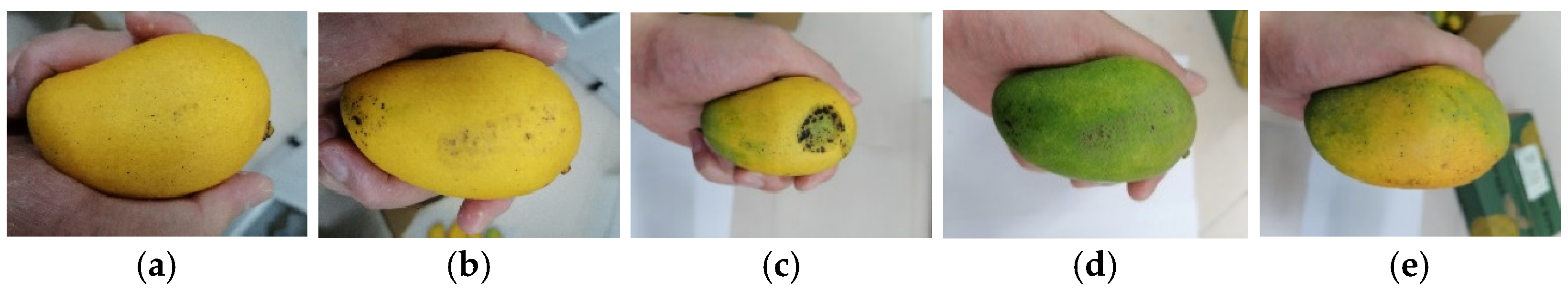
2.1. Experimental Materials

The dataset used in this study consists of 381 mango (Mangifera indica Linn, Tainong No.1) images taken by Huawei Honor Play3 mobile phone with a 12 megapixel sensor. According to industry standards, pictures were divided into five categories: Figure 1a–e. The judgement basis—shown in Figure 1. Figure 1a,d,e—involves mangoes of different maturities, while Figure 1b,c have different defects.
A data-augmentation method was employed to expand the number of images and improve the robustness of the deep-learning model [27,28]. As shown in Table 1, the original images were rotated by 90°, 180°, and 270°, and were cropped to 224 × 224 pixels; a total of 1524 images were obtained, which were divided into 1226 training samples and 298 test samples.

2.2. Experimental Platform

The experimental platform consists of cloud-computing and local development platforms [29,30,31]. As shown in Figure 2, after professional data annotation, the images were uploaded to the cloud-computing platform; then, the model was obtained after training and testing, and finally downloaded to the local application. The cloud computer was configured with an Intel Core i7-8750h CPU and NVDIA P100 GPU with 16 GB of memory. The local development platform was the Pytorch deep-learning framework running on the Windows 10 operating system; the programming language used was Python.

2.3. Model Evaluation Methods

Accuracy, precision, recall, and F1 value [32] were used to evaluate the effectiveness of the model. Since the experiment is a five-category experiment, each category is regarded as a positive category in turn, and the other categories are regarded as negative categories. The calculation formula of each index is as follows:
A P ( A v e r a g e   p r e c i s i o n ) = 1 k i = 1 k T P i T P i + F P i × 100 % .
A R ( A v e r a g e   r e c a l l ) = 1 k i = 1 k T P i T P i + F N i × 100 % .
F 1 = 2 × A P × A R A P + A R × 100 %
A c c u r a c y = T P + T N T P + T N + F P + F N × 100 %
where TP represents the number of positive samples correctly identified as positive samples, TN the number of negative samples correctly identified as negative samples, FP the number of negative samples incorrectly identified as positive samples, FN the number of positive samples incorrectly identified as negative samples, k the number of levels, and i the level itself.

2.4. Model Visualization

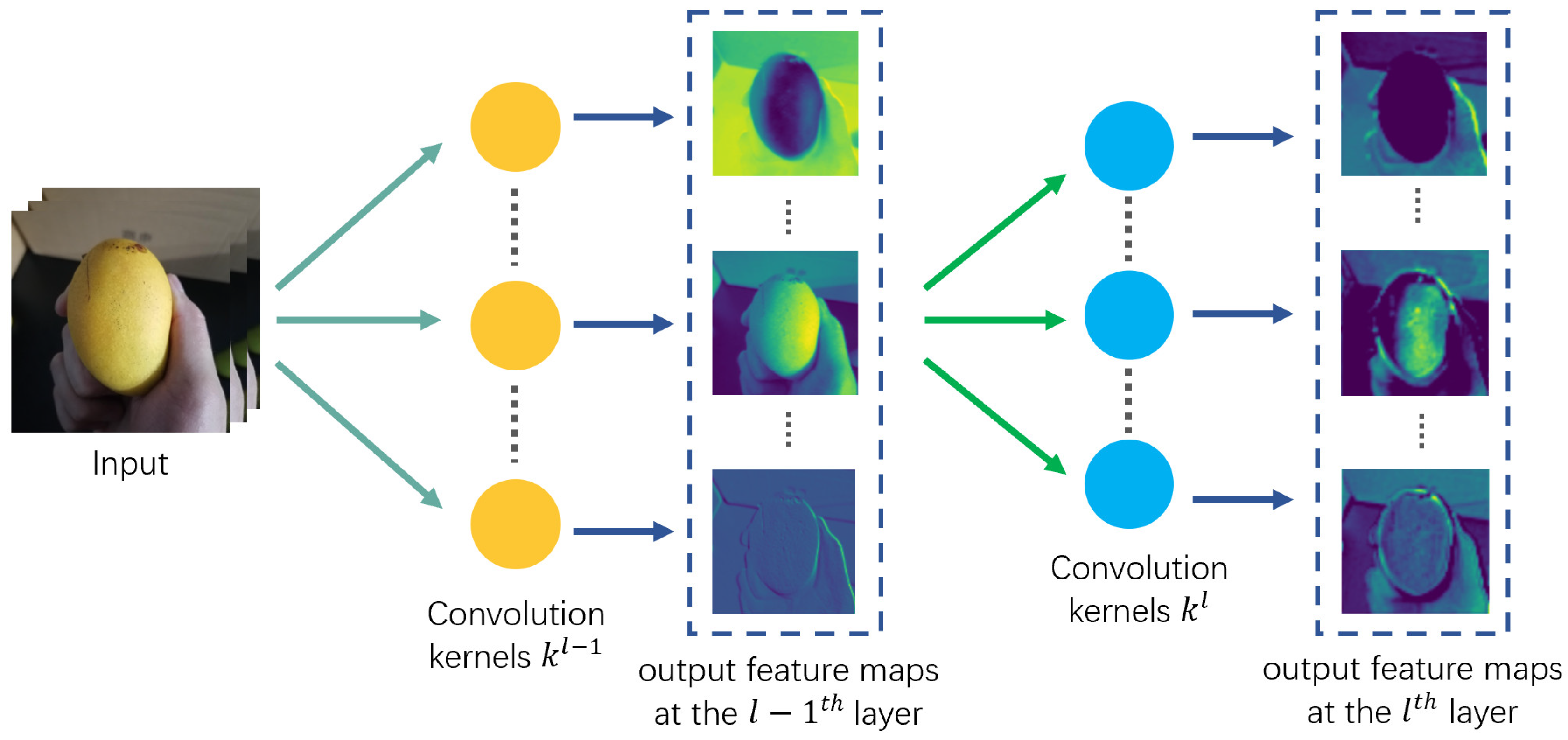
2.4.1. Convolution-Layer Visualization

It is necessary to understand the internal working mechanism of a model to improve its structure [33]. In our research, the feature maps of all channels were visualized, which allowed us to easily judge the performance of each filter, and each layer of the network contains multiple filters. The method is shown in Figure 3. The input image f ( x , y ) passes through the filters and then outputs feature maps. Each feature map corresponds to an independent feature, which is determined by the corresponding filter. The formula is
x j l = f ( i M x i l 1 × k i j + b j l )
where x i l 1 is the i t h input feature map at the ( l 1 ) t h layer, x j l is the j t h output feature map at the l th layer, and M is the set of feature maps at the ( l 1 ) t h layer. k i j l is the convolution kernel between the l t h input map at the layer ( l 1 ) t h and the j t h output map at layer l . b j l is the bias of the j t h output map at the l t h layer.

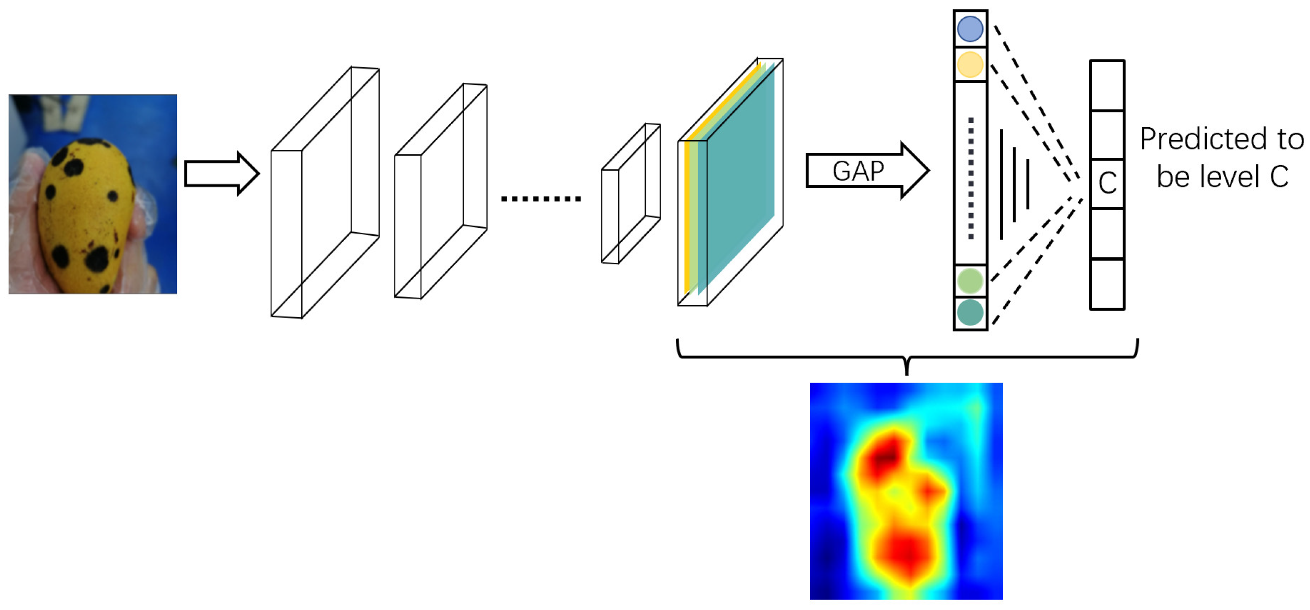
2.4.2. Feature Visualization

The CAM [34] method is a weighted linear sum of visual patterns at different spatial locations that can help us clearly determine which areas of an image the network pays more attention to. By matching the CAM with the input image, the area most relevant to a specific level can be identified. In the present work, the weight of the gap to the output layer was fully connected to the target category. Figure 4 is a CAM for a C-level mango. Since the gap feature vector comes directly from the feature map, this weight can be regarded as the contribution of the feature map to the target category score. The higher the score, the higher the contribution of the corresponding region of the original image to the network. The CAM can be obtained by the following formula:
M c ( x , y ) = k w k c f k ( x , y )
where f k ( x , y ) is the value of the position ( x , y ) of the last layer feature map and w k C the full connection weight of category C.

3. Model Construction and Training

3.1. Classic SqueezeNet

SqueezeNet is a lightweight and efficient convolutional-neural-network CNN model proposed by Han et al. [35]. In distributed training, SqueezeNet has fewer parameters and less communication with the server, which makes it more suitable for deployment on devices with limited memory, such as field-programmable gate arrays.
As shown in Figure 5, there is a convolution layer at the beginning and end of SqueezeNet, with eight fire modules and three max-pooling layers in the middle. When passing through a pooling layer, the image size is compressed to half of the original to reduce the amount of calculation. The last convolutional layer is 1 × 1 with 512 input channels and 1000 output channels, and the output image size is 14 × 14 pixels. The output of a convolution layer is pooled by the global average, and the probability of 1000 classifications is calculated by softmax.

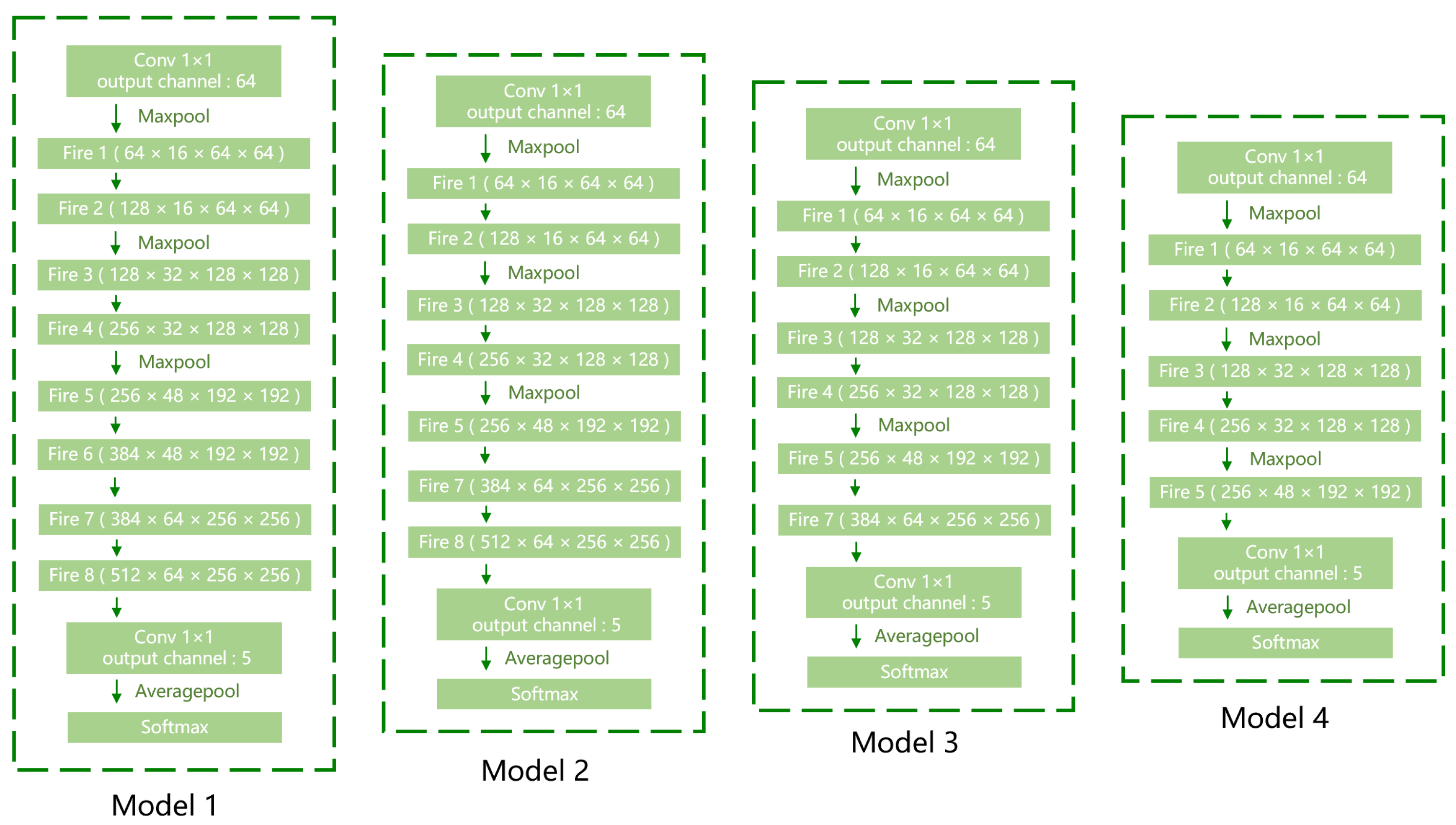
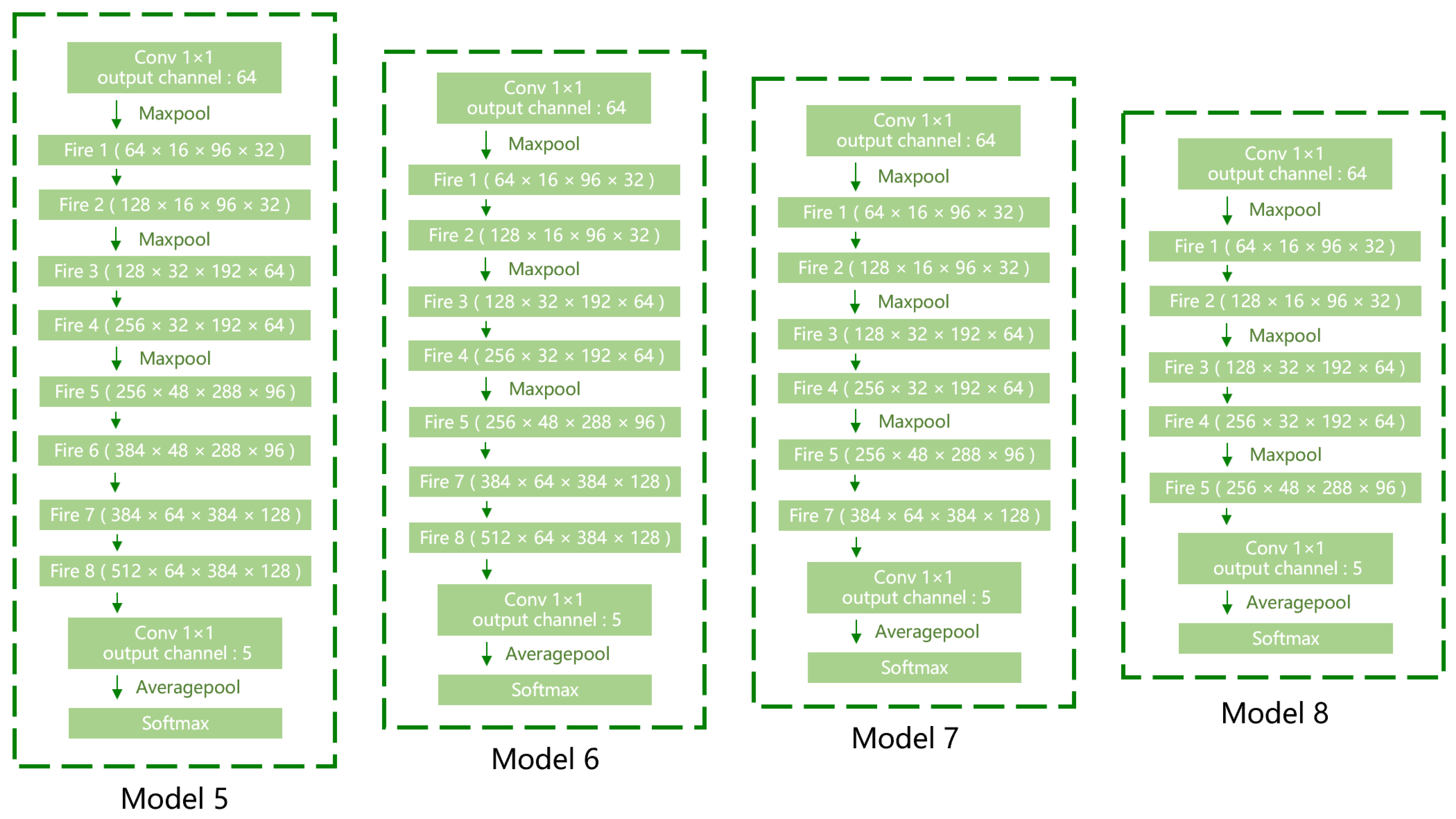
3.2. Network-Structure Modification

Figure 6 shows the visualization results of the convolution-layer features. The first fire module consisted of the collection of various edge detectors, and most of the information in the original image was retained at this time. The second fire module began to extract texture details, and feature maps became increasingly more abstract with the deepening of the layers and the increasing number of channels. The third and fourth fire modules paid more attention to local information, such as defects and shapes. However, the sparsity of activation increased with the layer from the sixth fire module, and increasingly more feature maps were blank [36]. This means that the patterns encoded by these filters cannot be found in the input image, and these inactivated feature maps cannot provide effective information. Therefore, the layers containing more blank information can be removed to compress the model.
Since only five categories of mangoes must be identified, the number of output channels of the convolution layer was modified to five, which was recorded as Model 1. Considering the simple characteristics of a mango, too much overall information was unnecessary. According to the visualization results, the last three fire modules showed great similarity, and the number of activated feature maps gradually decreased, which indicated that these feature maps are redundant and can be removed. As shown in Figure 7, fire Modules 6–8 were removed from the original model and denoted Models 2–4, respectively.

3.3. Fire-Module Modification
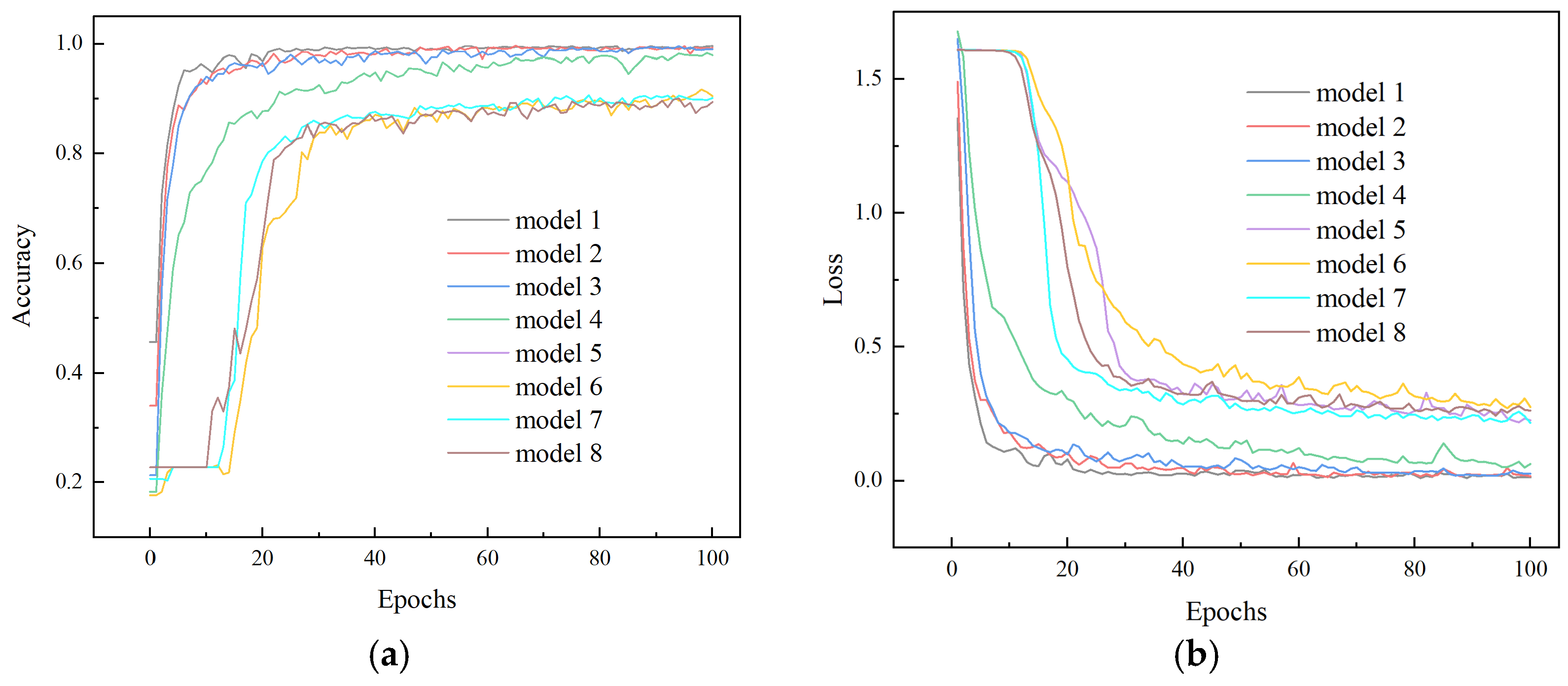
As shown in Figure 8, the core of SqueezeNet is the fire module, which is composed of two parts: the squeeze and expand layers. The squeeze layer is a 1 × 1 convolution kernel, which changes the input channel from M to N; N is usually less than M. The squeeze layer is mainly used to compress the input channel to reduce the amount of calculation of the network.
The expansion layer contains two types of convolution kernels, i.e., 1 × 1 and 3 × 3. These two convolution kernels expand the input channel from N to E1 and E2, respectively. The obtained feature map is spliced to obtain the characteristic map with an output channel (E1 + E2).
Since the 3 × 3 convolution kernel of a fire module has nine parameters in total, nine floating-point multiplications and one floating-point addition are required for one convolution. However, the 1 × 1 convolution kernel has only one parameter, and only one floating-point multiplication is required for one convolution operation. Therefore, the convolution operations and parameter amounts of 1 × 1 are approximately one-ninth of that of the 3 × 3 convolution.
Based on this principle, the partial 3 × 3 convolution kernel was replaced by the 1 × 1 convolution kernel, which can not only reduce the number of parameters but also greatly reduce the degree of calculation. As shown in Figure 9, the convolution kernels of the fire modules in Models 1–4 were redistributed with a ratio of 3:1 to obtain Models 5–8.

3.4. Model Training

Transfer learning was used to accelerate the model convergence [37] and the Adam optimizer was used [38]. The improved models were pre-trained on the Imagenet dataset, and the pre-training weights were taken as the initial value of the initial kernel. The ReLu function was used as an activation function. The cross-entropy loss function was selected to deal with the class-imbalanced dataset. The loss caused by the category with a small sample number was given a large weight, while the loss caused by the category with a large sample number was given a small one. This can reduce the loss value and improve the robustness of the mode. The learning rate was 0.0001, the batch size was 128, and the number of iterations was 100. Figure 10 shows the training results.
As shown in Figure 10, the accuracy curves of Models 1–4 began to converge in the tenth round, and the final accuracy rate stabilized at more than 90%, while the accuracy curves of Models 5–8 began to converge in the 30th round, and the final accuracy was stable at more than 85%. Overall, although the convergence speed of each model was different, the loss value could be stable at a lower value after 50 iterations.

4. Results and Discussion

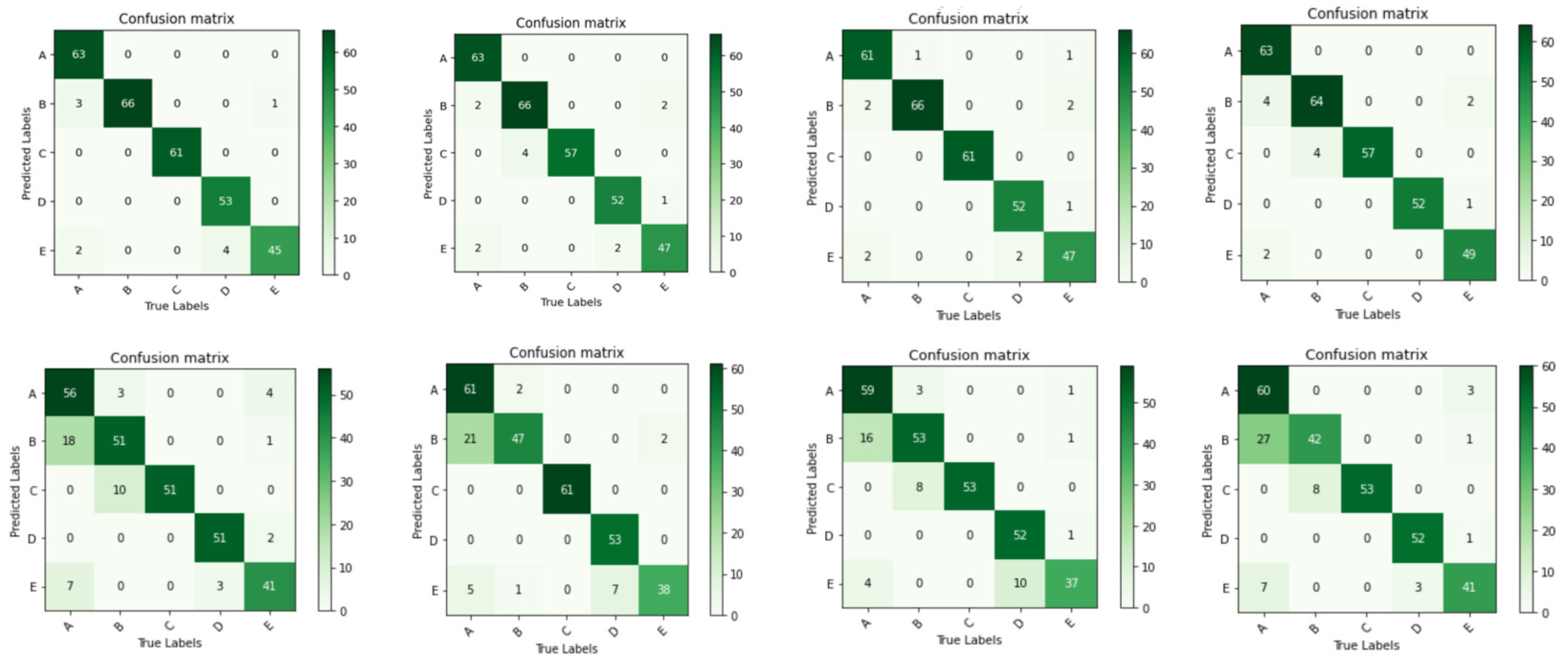
4.1. Model Test and Evaluation

Figure 11 is the confusion matrix [39] of Models 1–8 on the test set and was used to explore the performance of each model. Regarding appearance quality, there was no misjudgment between Levels A and C, but a small amount of Level B was misjudged. Among the eight models, the lowest misjudgment rate of Level B was 2.86%, and the highest was 38.57%. Regarding maturity, there was no misjudgment between mature and immature mangoes, but partially mature mangoes might have been misjudged; the lowest misjudgment rate was 3.92%, and the highest was 27.45%. The above phenomena were similar to those observed in manual sorting.
Level A represents a first-class mango, B a second-class mango, C a third-class mango, D an immature mango, and E a partially mature mango.
Table 2 shows the parameters and performance of all models. It can be seen that Model 1 had the highest F1 score, but its parameter memory requirements and the amount of computation required by the model were the largest among all models, reaching 2.78 MB and 265.48 MFLOPS, respectively. It can be seen from the trend that the two indicators from Models 1 to 4 decrease in turn, but the F1 score does not change significantly, which shows that the deep network has little positive impact on mango sorting. Upon comparison with Models 1–4, the parameter memory requirements and amount of computation required for Models 5–8 were greatly improved, but the test accuracy was not satisfactory. This shows that adjusting the number of 1 × 1 and 3 × 3 convolution cores in the expansion layer can effectively improve the parameter memory and computation requirements, but it comes at the expense of performance. Therefore, Model 4 has the best performance among all models, with an average accuracy of 95.64%, and its parameter memory and computation requirements are 0.87 MB and 181.34 MFLOPS, respectively.
To verify the practicability of Model 4, the test set was divided into two groups: one for maturity and the other for appearance quality (the results are shown in Table 3). The test accuracy on the two datasets reached more than 95%, and the accuracy of maturity was 2.37% higher than that of appearance quality. It can be seen that the model shows a good generalizability and strong robustness.

4.2. Comparison with Classical Models

Model 4 was compared with the classic deep networks AlexNet [40], VGG [41], ResNet [42], GoogleNet [43], DenseNet [44], MobileNet [45], Vision Transformers (ViT) [46], and EfficientNet [47] to facilitate a more objective and comprehensive evaluation; the results are shown in Table 4. Although the accuracy of ViT-B/16 is 97.17%, its parameter memory requirements and amount of computation required are much higher than that of Model 4. It also can be seen that the proposed Model 4 has a better cost performance and competitive advantages. Even the classical model MobileNet, which has the smallest parameter storage, has almost 10 times the parameter memory and 10 times as many computation requirements as Model 4. Model 4, however, saves a significant number of computational resources, and its accuracy can still be maintained at 95.64%.

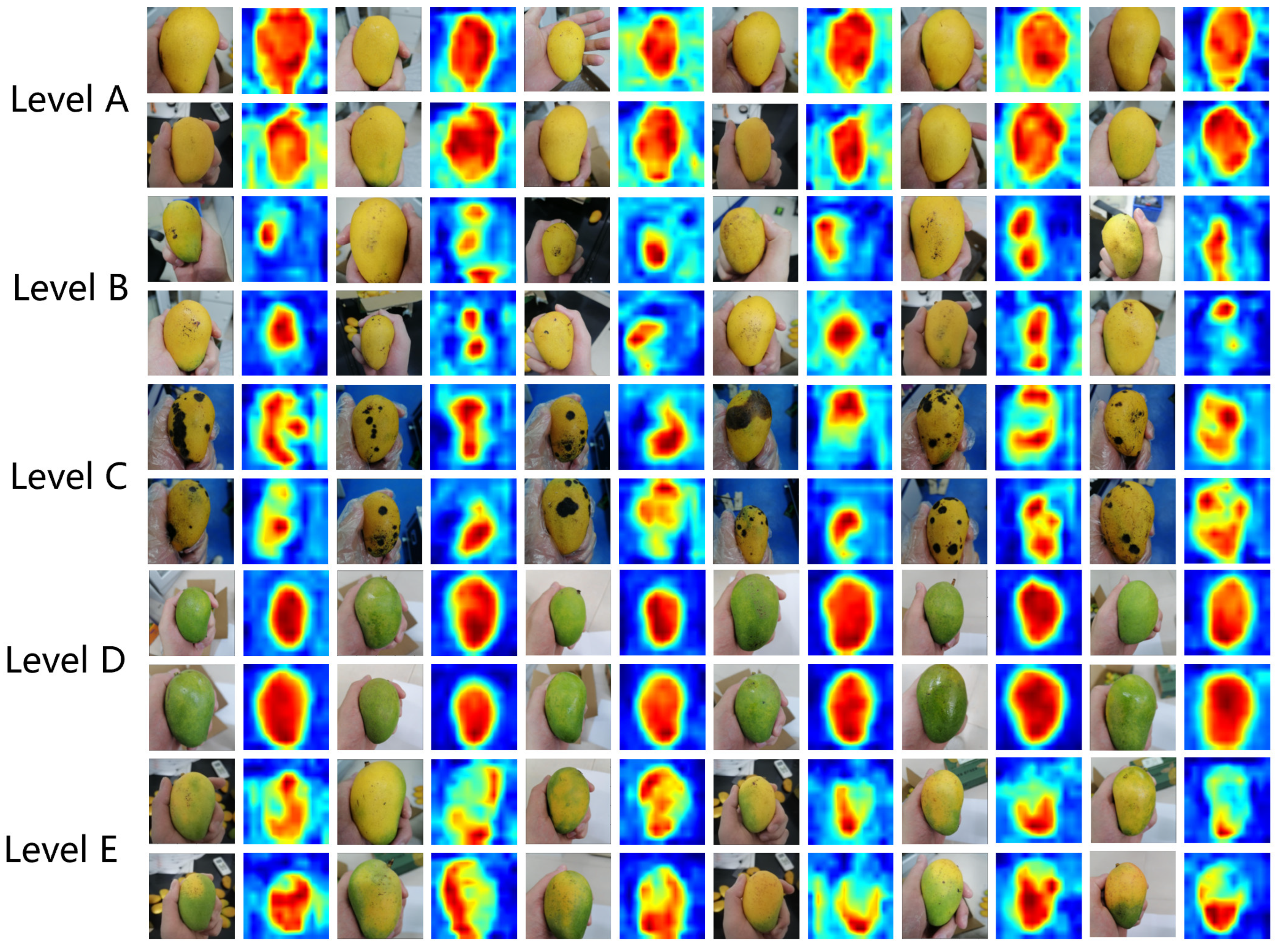
4.3. Visual Output Analysis of Model

Figure 12 displays the CAM of the different mango levels. The value of each pixel on the image can be understood as the contribution to the predicted result. It can be seen that Levels A and D focus on the whole mango, and the result is not disturbed by the background. The judgment of Levels B and C focuses on defects, and the distribution of heat depends on the defects’ location and range. For Level E, the attention of the model is mainly attracted by the color change. These results are completely consistent with the judgment standard for mangoes of various levels, which shows that the model has good practicability.

5. Conclusions

In this study, the feature-extraction characteristics of the shallow and deep networks of the SqueezeNet model were analyzed by a visualization method, and eight extrusion network models were constructed based on the results. After the training and evaluation, it was found that Model 4 exhibited the best performance among the other models, with an accuracy of 95.64% and an F1 score of 0.9587. The parameter memory requirements and computation required by the model were only 0.87 MB and 181.34 MFLOPS, respectively. The model performed well with respect to the mangoes’ appearance and maturity classification experiments. Compared with the classical AlexNet, VGG16, VGG11, ResNet18, ResNet34, GoogleNet, DenseNet, and MobileNet models, the proposed Model 4 significantly lowered the computing power required without reducing its accuracy. Through a CAM analysis, it was found that for mangoes in Levels B and C, the model paid more attention to surface defects, while for Level E, color change was the primary factor. For other mango levels, the entire surface had almost the same effect on the discrimination results, which was consistent with the judgment standards of all the kinds of mango. Therefore, the proposed model was more suitable for embedded-resource-constrained devices such as mobile terminals and it showed a higher cost performance in comparison with existing models.

Author Contributions

Methodology, H.W., L.Z. and Z.M.; software, W.C. and X.C.; validation, Y.M. and H.L.; data curation, W.C. and X.C.; writing—original draft preparation, H.W. and W.C.; writing—review and editing, H.W., L.Z. and Z.M.; supervision, L.Z.; project administration, Z.M.; funding acquisition, H.W. All authors have read and agreed to the published version of the manuscript.

Funding

This research was funded by Guangdong Provincial Agricultural Science and Technology Innovation and Extension Project, grant number 2022KJ101 and 2022KJ131, and National key research and development projects during the “14th five year plan”, grant number 2021YFD2000701-03.

Institutional Review Board Statement

Not applicable.

Data Availability Statement

The data presented in this study are available on request from the corresponding author.

Acknowledgments

We thank LetPub (www.letpub.com (accessed on 10 August 2022)) for its linguistic assistance during the preparation of this manuscript.

Conflicts of Interest

The authors declare no conflict of interest.

References

  1. Lebaka, V.R.; Wee, Y.J.; Ye, W.; Korivi, M. Nutritional Composition and Bioactive Compounds in Three Different Parts of Mango Fruit. Int. J. Environ. Res. Public Health 2021, 18, 741. [Google Scholar] [CrossRef] [PubMed]
  2. Thakur, R.; Suryawanshi, G.; Patel, H.; Sangoi, J. An innovative approach for fruit ripeness classification. In Proceedings of the 2020 4th International Conference on Intelligent Computing and Control Systems (ICICCS), Madurai, India, 13–15 May 2020; pp. 550–554. [Google Scholar]
  3. Qiao, Q. Image Processing Technology Based on Machine Learning. IEEE Consum. Electron. Mag. 2022. [Google Scholar] [CrossRef]
  4. Liu, L.; Wang, Y.; Chi, W. Image Recognition Technology Based on Machine Learning. IEEE Access 2020. [Google Scholar] [CrossRef]
  5. Truong Minh Long, N.; Truong Thinh, N. Using Machine Learning to Grade the Mango’s Quality Based on External Features Captured by Vision System. Appl. Sci. 2020, 10, 5775. [Google Scholar] [CrossRef]
  6. Nandi, C.S.; Tudu, B.; Koley, C. A Machine Vision Technique for Grading of Harvested Mangoes Based on Maturity and Quality. IEEE Sens. J. 2016, 16, 6387–6396. [Google Scholar] [CrossRef]
  7. Pise, D.; Upadhye, G.D. Grading of harvested mangoes quality and maturity based on machine learning techniques. In Proceedings of the 2018 International Conference on Smart City and Emerging Technology (ICSCET), Mumbai, India, 5 January 2018; pp. 1–6. [Google Scholar]
  8. Kumar, P.R.; Manash, E.B.K. Deep learning: A branch of machine learning. J. Phys. Conf. Ser. 2019, 1228, 012045. [Google Scholar] [CrossRef]
  9. Naranjo-Torres, J.; Mora, M.; Hernández-García, R.; Barrientos, R.J.; Fredes, C.; Valenzuela, A. A Review of Convolutional Neural Network Applied to Fruit Image Processing. Appl. Sci. 2020, 10, 3443. [Google Scholar] [CrossRef]
  10. Aherwadi, N.; Mittal, U. Fruit quality identification using image processing, machine learning, and deep learning: A review. Adv. Appl. Math. Sci. 2022, 21, 2645–2660. [Google Scholar]
  11. Snatkina, O.A.; Kugushev, A.R. Determination of fruit quality by image using deep neural network. In Proceedings of the 2022 Conference of Russian Young Researchers in Electrical and Electronic Engineering (ElConRus), St. Petersburg, Russia, 25–28 January 2022; pp. 1423–1426. [Google Scholar]
  12. Yang, H.; Wen, T.; Yang, X.; Lin, H. Deep Learning Agricultural Information Classification Combined with Internet of Things Technology in Agricultural Production and Economic Management. IEEE Access 2022, 10, 54713–54719. [Google Scholar] [CrossRef]
  13. Hossain, M.S.; Al-Hammadi, M.; Muhammad, G. Automatic Fruit Classification Using Deep Learning for Industrial Applications. IEEE Trans. Ind. Inform. 2019, 15, 1027–1034. [Google Scholar] [CrossRef]
  14. Wu, S.-L.; Tung, H.-Y.; Hsu, Y.-L. Deep learning for automatic quality grading of mangoes: Methods and insights. In Proceedings of the 2020 19th IEEE International Conference on Machine Learning and Applications (ICMLA), Miami, FL, USA, 14–17 December 2020; pp. 446–453. [Google Scholar]
  15. Rizwan Iqbal, H.M.; Hakim, A. Classification and Grading of Harvested Mangoes Using Convolutional Neural Network. Int. J. Fruit Sci. 2022, 22, 95–109. [Google Scholar] [CrossRef]
  16. Tripathi, M.K.; Maktedar, D.D. Optimized deep learning model for mango grading: Hybridizing lion plus firefly algorithm. IET Image Process. 2021, 15, 1940–1956. [Google Scholar] [CrossRef]
  17. Huang, J.; Lu, X.; Chen, L.; Sun, H.; Wang, S.; Fang, G. Accurate Identification of Pine Wood Nematode Disease with a Deep Convolution Neural Network. Remote Sens. 2022, 14, 913. [Google Scholar] [CrossRef]
  18. Aqil, M.; Azrai, M.; Mejaya, M.J.; Subekti, N.A.; Tabri, F.; Andayani, N.N.; Wati, R.; Panikkai, S.; Suwardi, S.; Bunyamin, Z.; et al. Rapid Detection of Hybrid Maize Parental Lines Using Stacking Ensemble Machine Learning. Appl. Comput. Intell. Soft Comput. 2022, 2022, 6588949. [Google Scholar] [CrossRef]
  19. Naik, B.N.; Malmathanraj, R.; Palanisamy, P. Detection and classification of chilli leaf disease using a squeeze-and-excitation-based CNN model. Ecol. Inform. 2022, 69, 101663. [Google Scholar] [CrossRef]
  20. Chen, X.; Sun, Z.-L.; Chen, X. A machine learning based automatic tomato classification system. In Proceedings of the 2021 33rd Chinese Control and Decision Conference (CCDC), Kunming, China, 22–24 May 2021; pp. 5105–5108. [Google Scholar]
  21. Zheng, B.; Huang, T.; Houssein, E. Mango Grading System Based on Optimized Convolutional Neural Network. Math. Probl. Eng. 2021, 2021, 2652487. [Google Scholar] [CrossRef]
  22. Liang, J.; Zhang, T.; Feng, G. Channel Compression: Rethinking Information Redundancy Among Channels in CNN Architecture. IEEE Access 2020, 8, 147265–147274. [Google Scholar] [CrossRef]
  23. Liu, Y.; Gao, G. Identification of multiple leaf diseases using improved SqueezeNet model. Trans. Chin. Soc. Agric. Eng. 2021, 37, 187–195. [Google Scholar]
  24. Lipton, Z.C. The mythos of model interpretability: In machine learning, the concept of interpretability is both important and slippery. Queue 2018, 16, 31–57. [Google Scholar] [CrossRef]
  25. Adadi, A.; Berrada, M. Peeking Inside the Black-Box: A Survey on Explainable Artificial Intelligence (XAI). IEEE Access 2018, 6, 52138–52160. [Google Scholar] [CrossRef]
  26. Selvaraju, R.R.; Das, A.; Vedantam, R.; Cogswell, M.; Parikh, D.; Batra, D. Grad-CAM: Why did you say that? arXiv 2016, arXiv:1611.07450. [Google Scholar]
  27. Perez, L.; Wang, J. The effectiveness of data augmentation in image classification using deep learning. arXiv 2017, arXiv:1712.04621. [Google Scholar]
  28. Baird, H.S.; Bunke, H.; Wang, P.S.-P. Document Image Analysis; World Scientific Publishing Company: Los Alamitos, CA, USA, 1994. [Google Scholar]
  29. Luckow, A.; Cook, M.; Ashcraft, N.; Weill, E.; Djerekarov, E.; Vorster, B. Deep learning in the automotive industry: Applications and tools. In Proceedings of the 2016 IEEE International Conference on Big Data (Big Data), Washington, DC, USA, 5–8 December 2016; pp. 3759–3768. [Google Scholar]
  30. Shaukat, Z.; Farooq, Q.U.A.; Tu, S.; Xiao, C.; Ali, S. A state-of-the-art technique to perform cloud-based semantic segmentation using deep learning 3D U-Net architecture. BMC Bioinform. 2022, 23, 251. [Google Scholar] [CrossRef] [PubMed]
  31. Carneiro, T.; Da Nobrega, R.V.M.; Nepomuceno, T.; Bian, G.-B.; de Albuquerque, V.H.C.; Filho, P.P.R. Performance Analysis of Google Colaboratory as a Tool for Accelerating Deep Learning Applications. IEEE Access 2018, 6, 61677–61685. [Google Scholar] [CrossRef]
  32. Hand, D.; Christen, P. A note on using the F-measure for evaluating record linkage algorithms. Stat. Comput. 2018, 28, 539–547. [Google Scholar] [CrossRef]
  33. Qin, Z.; Yu, F.; Liu, C.; Chen, X. How convolutional neural networks see the world—A survey of convolutional neural network visualization methods. Math. Found. Comput. 2018, 1, 149–180. [Google Scholar] [CrossRef]
  34. Selvaraju, R.R.; Cogswell, M.; Das, A.; Vedantam, R.; Parikh, D.; Batra, D. Grad-cam: Visual explanations from deep networks via gradient-based localization. In Proceedings of the IEEE International Conference on Computer Vision, Venice, Italy, 22–29 October 2017; pp. 618–626. [Google Scholar]
  35. Iandola, F.N.; Han, S.; Moskewicz, M.W.; Ashraf, K.; Dally, W.J.; Keutzer, K. SqueezeNet: AlexNet-level accuracy with 50x fewer parameters and <0.5 MB model size. arXiv 2016, arXiv:1602.07360. [Google Scholar]
  36. Chollet, F. Deep Learning with Python; Simon and Schuster: Berkeley, CA, USA, 2021. [Google Scholar]
  37. Zhuang, F.; Qi, Z.; Duan, K.; Xi, D.; Zhu, Y.; Zhu, H.; Xiong, H.; He, Q. A comprehensive survey on transfer learning. Proc. IEEE 2020, 109, 43–76. [Google Scholar] [CrossRef]
  38. Bock, S.; Weiß, M. A proof of local convergence for the Adam optimizer. In Proceedings of the 2019 International Joint Conference on Neural Networks (IJCNN), Budapest, Hungary, 14–19 July 2019; pp. 1–8. [Google Scholar]
  39. Barranco-Chamorro, I.; Carrillo-García, R.M. Techniques to Deal with Off-Diagonal Elements in Confusion Matrices. Mathematics 2021, 9, 3233. [Google Scholar] [CrossRef]
  40. Krizhevsky, A.; Sutskever, I.; Hinton, G.E. Imagenet classification with deep convolutional neural networks. In NIPS’12: Proceedings of the 25th International Conference on Neural Information Processing Systems, Lake Tahoe, Nevada, 3–6 December 2012; Curran Associates Inc.: Red Hook, NY, USA, 2012. [Google Scholar]
  41. Ewe, E.L.R.; Lee, C.P.; Kwek, L.C.; Lim, K.M. Hand Gesture Recognition via Lightweight VGG16 and Ensemble Classifier. Appl. Sci. 2022, 12, 7643. [Google Scholar] [CrossRef]
  42. He, K.; Zhang, X.; Ren, S.; Sun, J. Deep residual learning for image recognition. In Proceedings of the IEEE Conference on Computer Vision and Pattern Recognition, Las Vegas, NV, USA, 26 June–1 July 2016; pp. 770–778. [Google Scholar]
  43. Szegedy, C.; Vanhoucke, V.; Ioffe, S.; Shlens, J.; Wojna, Z. Rethinking the inception architecture for computer vision. In Proceedings of the IEEE Conference on Computer Vision and Pattern Recognition, Las Vegas, NV, USA, 26 June–1 July 2016; pp. 2818–2826. [Google Scholar]
  44. Huang, G.; Liu, Z.; van der Maaten, L.; Weinberger, K.Q. Densely connected convolutional networks. In Proceedings of the IEEE Conference on Computer Vision and Pattern Recognition, Honolulu, HI, USA, 21–26 July 2017; pp. 4700–4708. [Google Scholar]
  45. Howard, A.G.; Zhu, M.; Chen, B.; Kalenichenko, D.; Wang, W.; Weyand, T.; Andreetto, M.; Adam, H. Mobilenets: Efficient convolutional neural networks for mobile vision applications. arXiv 2017, arXiv:1704.04861. [Google Scholar]
  46. Dosovitskiy, A.; Beyer, L.; Kolesnikov, A.; Weissenborn, D.; Zhai, X.; Unterthiner, T.; Dehghani, M.; Minderer, M.; Heigold, G.; Gelly, S.; et al. An image is worth 16x16 words: Transformers for image recognition at scale. arXiv 2020, arXiv:2010.11929. [Google Scholar]
  47. Tan, M.; Le, Q. Efficientnet: Rethinking model scaling for convolutional neural networks. In Proceedings of the International Conference on Machine Learning, Long Beach, CA, USA, 9–15 June 2019; pp. 6105–6114. [Google Scholar]
Figure 1. Different levels of mango samples. Level A has almost no defects and its greenness is less than 20%; Level B’s defects are less than 10%; Level C’s defects are more than 10%; Level D has almost no defects and its greenness is more than 70%; Level E has almost no defects and its greenness is between 20~70%. (a) Level A; (b) Level B; (c) Level C; (d) Level D; (e) Level E.
Agriculture 12 01467 g001
Figure 2. Deep-learning process.
Agriculture 12 01467 g002
Figure 3. Output feature maps of the middle layer of CNN.
Agriculture 12 01467 g003
Figure 4. CAM generation process.
Agriculture 12 01467 g004
Figure 5. Traditional SqueezeNet network structure.
Agriculture 12 01467 g005
Figure 6. Visualization results of convolution-layer features.
Agriculture 12 01467 g006
Figure 7. Network structure of Models 1–4.
Agriculture 12 01467 g007
Figure 8. Fire module structure. The fire module is defined as fire (M, N, E1, and E2), where M and N represent the number of input and output channels, respectively, of the squeeze layer. E1 and E2 represent the number of output channels of expand layer 1 × 1 and expand layer 3 × 3, respectively.
Agriculture 12 01467 g008
Figure 9. Network structure of Models 5–8.
Agriculture 12 01467 g009
Figure 10. Results of Models 1–8 on the training set: (a) Comparison of accuracy; (b) Comparison of loss values.
Agriculture 12 01467 g010
Figure 11. Confusion matrices of Models 1–8 on the test set.
Agriculture 12 01467 g011
Figure 12. CAM of different levels of mango.
Agriculture 12 01467 g012
Table 1. Sample assignment of training and test datasets.
LevelTraining SetTest Set
A25463
B27970
C25161
D21653
E22651
Total1226298
Table 2. Modified model parameters and performance.
ModelTest
Accuracy
(%)
Average Precision (%)Average Recall (%)F1 ScoreParameter Memory (MB)Computation
(MFLOPs)
Model 196.6496.5096.690.96592.78265.48
Model 295.6395.6095.720.95662.36246.72
Model 396.3196.2896.160.96221.60213.39
Model 495.6495.8195.930.95870.87181.34
Model 583.8984.3985.740.85061.85179.78
Model 687.2587.7089.490.88591.56169.67
Model 785.2385.3886.770.86071.05147.42
Model 883.2284.1386.300.85200.58126.44
Table 3. Maturity and appearance quality test results.
Test SetsClassificationPrecision (%)Recall (%)Accuracy (%)
Appearance qualityA100.0094.0295.83
B91.4294.12
C93.44100.00
MaturityA100.0096.9298.20
D98.11100.00
E96.0898.00
Table 4. Performance comparisons of proposed Model 4 with classical models.
ModelAccuracy (%)Parameter Memory (MB)Computation
(MFLOPs)
AlexNet92.2827.90660.90
VGG1696.64105.6515,483.86
VGG1196.3084.77616.57
ResNet1894.3543.221818.69
ResNet3496.0181.843670.88
GoogleNet95.0122.071503.86
DenseNet96.6729.622865.30
MobileNet93.358.74312.86
ViT-B/1697.17327.3734,529.28
EfficientNet89.3415.6327.02
Model 495.640.87181.34
Publisher’s Note: MDPI stays neutral with regard to jurisdictional claims in published maps and institutional affiliations.

