Article

Investigating the Material Properties of Nodular Cast Iron from a Data Mining Perspective

by
Cristiano Fragassa
Department of Industrial Engineering, Alma Mater Studiorum University of Bologna, Viale del Risorgimento 2, 40136 Bologna, Italy
Metals 2022, 12(9), 1493; https://doi.org/10.3390/met12091493
Submission received: 11 August 2022 / Revised: 1 September 2022 / Accepted: 7 September 2022 / Published: 9 September 2022
(This article belongs to the Section Metal Casting, Forming and Heat Treatment)

Abstract

:
Cast iron is a very common and useful metal alloy, characterized by its high carbon content (>4%) in the allotropic state of graphite. The correct shape and distribution of graphite are essential for ensuring that the material has the right properties. The present investigation examines the metallurgical and mechanical characterization of a spheroidal (nodular) cast iron, an alloy that derives its name and its excellent properties from the presence of graphite as spheroidal nodules. Experimental data are detected and considered from a data mining perspective, with the scope to extract new and little-known information. Specifically, a machine learning toolkit (i.e., Orange Data Mining) is used as a means of permitting supervised learners/classifiers (such as neural networks, k-nearest neighbors, and many others) to understand related metallurgical and mechanical features. An accuracy rate of over 90% can be considered as representative of the method. Finally, interesting considerations emerged regarding the dimensional effect on the variation in the solidification rates, microstructure, and properties.

1. Introduction

Data mining traditionally represents the identification of information, not known a priori, through targeted extrapolation using single or multiple databases. Techniques and strategies applied to data mining operations are largely automated and frequently based on machine learning (ML) algorithms.
To date, prediction methods, such as neural networks, decision trees, clustering, regression and the analysis of associations, are commonly used in material engineering. With the capacity to recognize existing patterns undetected by other means of investigation, they can provide unforeseen information in a way that permits a better understanding of material properties and behaviors. This is exactly what it is presented here, with an investigation focused on a nodular cast iron (GJS).
Also known as spheroidal graphite cast iron (SGI), this is a standardized [1] type of cast iron in which graphite is solidified as spheroids (instead of flakes or lamellae), with the effect of providing the material with better mechanical properties (e.g., ultimate/yield strength, hardness, etc.). They also provide properties that are rarely associated with cast irons, such as the ductility, which explains the further denomination of ductile iron [2].
The nodules of graphite exert a preventative action against the development of cracks, unlike lamellar graphite, which offers a preferential path for their propagation. In addition, their spheroidal shape reduces the stress concentration, reducing the damage in the matrix structure [3].
The intense influence exercised by the graphite shape on the matrix structure produces significant correlations between the mechanical properties. It is very common, e.g., to have tensile strength (UTS) correlated with elongation at break (ε) in the case of SGI, by means of an equation such as:
UTS2 × ε = Q
where Q is a constant. High values of Q indicate a high strength and/or elongation, denoting a cast iron with advanced properties [4].
The proper nucleation of the graphite spheroids AIn be achieved by combining two phases: firstly, by reducing the sulfur (S) content below 0.018% through a desulfurization treatment, and then, by increasing the magnesium (Mg) content up to 0.3% from its 0.04–0.05% initial content through the addition of Fe-Si-Mg alloys to the liquid metal ([5]). This a delicate part of the process.
There are equations (e.g., those proposed by CTIF and ESF, France) that can relate the weight of Mg-based additives with the expected Mg content. However, these relationships can be inaccurate. For instance, the desulfurization pre-treatment is essential for preventing the Mg from reacting, to a large extent, with the sulfur, hindering the complete spheroidization of the graphite. However, the local sulfur content can be influenced by the casting geometry and characteristic dimensions in a way that causes the microstructures to be unpredictable.
From a research perspective, this unpredictability is a perfect way of assessing data mining tools and their benefits, provided that we have adequate data for their analyses.
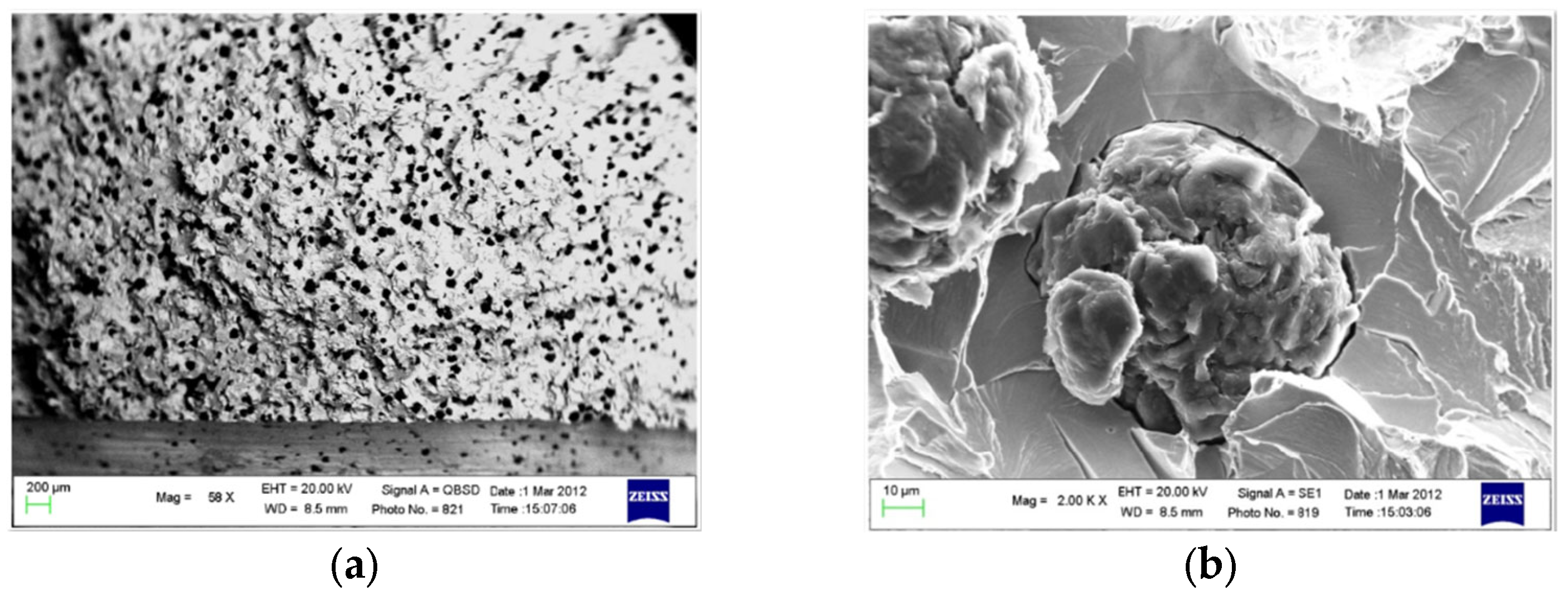
The distribution and morphology of graphite nodules can be detected using qualitative methods based on metallography. For instance, their shape can be evaluated according to ASTM A247, which defines seven basic morphologies and also provides parameters for their classification [6], before other standards are used to define specific tests methods.
The nodularity, which refers to the % of graphite present as type-I or -II nodules, can be evaluated by counting the graphite particles of each type [7]. A nodularity greater than 90% is generally recommended in the case of nodular iron, although a nodularity greater than 80% is acceptable.
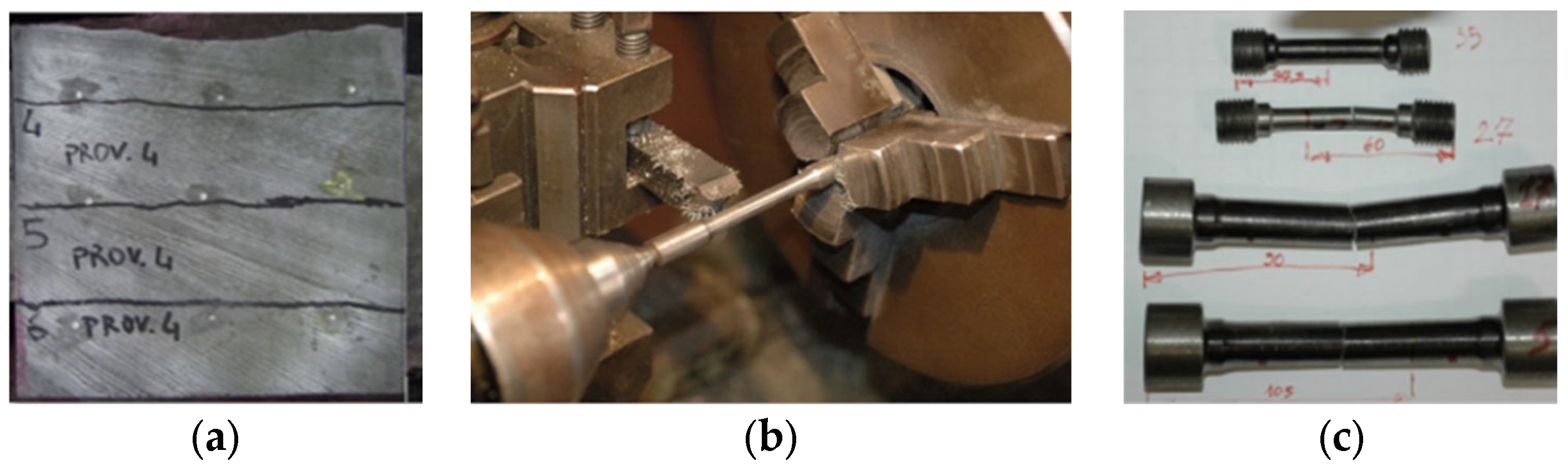
The mechanical properties can be evaluated using a consolidated list of standards merging experimental procedures for testing metallic materials (e.g., ASTM E8M-16 for tensile tests [8]) with other procedures that were explicitly developed for testing cast iron (e.g., ASTM A327 for impact tests of cast iron [9]).
There are numerous experimental works characterizing spheroidal cast irons in the literature, including some studies regarding specimens produced in the same foundry using similar processes and chemical compositions [10,11,12]. These papers describe SGIs with a good carbon content (3.50–3.70%), correct fractions of magnesium (0.055%) and minimal residues of sulfur (0.004%), as one should expect. Moreover, their spheroids appear to be correctly formed and distributed, while mechanical tests highlight the typical mechanical properties of SGI (i.e., tensile strength (UTS) ~500–670 MPa, yield strength (YS) ~320–380 MPa, Poisson’s ratio~0.24, and elongation at break (ε) ~9–14%).
Starting from the experimental data, models have been proposed in the past by researchers who were attempting to correlate the microstructural and mechanical information. They are usually based on the deployment of empirical relations correlating measurements, followed by remarkable attempts to interpret these relationships on a physical basis (e.g., [13,14,15]).
However, recent promising studies have introduced the concept of data mining as a new method for investigating the complexity behind the experimental data for cast irons.
In [16], e.g., data mining was used to classify the microstructures (i.e., martensite, pearlite and bainite) in the case of two-phases steels. This work offers valuable considerations regarding methods for producing a pertinent dataset for a machine learning (ML) approach, starting with the morphological parameters (such as the nodule shape, areas and diameters) detected using micrographs (i.e., light-optical and SEM images). The analysis also provides evidence with respect to the high accuracy of classification that can be achieved (i.e., 88.3%) when aspects such as data preprocessing, feature selection and the data split technique are properly handled. In this case, a support vector machine (SVM) tool trained using 80% of the available data was used as the classifier, and the other 20% of the data were retained for the validation.
The present investigation is similar in terms of the methods used and precision achieved, but significant there are differences in terms of the materials (i.e., cast iron vs. steel), training dataset consistency, morphological features, the application of learners, validation approach, etc.
In [17], the same SVM learner was applied to classify the material phases for SGI, as in the present work. However, the analysis was not based on the determination of the morphology of spheroids (as was the case, e.g., in [18]). Rather, the authors preferred to omit a grayscale (8-bit) transformation and evaluation, opening up the concept of image embeddings [19].
Clustering and classification algorithms rarely work when using images directly. To perform the image analysis, it is necessary to transform (‘encode’) them into vectors of numbers. The image embedding is a vector representation of an image, whereby images with similar patterns have similar vector profiles.
Today, many powerful image embedders are easily accessible (e.g., InceptionV3 by Google) and applied in several research fields (including materials engineering [20]). They are based on deep learning models that are able to calculate a feature vector for the image and return the image descriptors. These descriptors, which are altogether capable of precisely characterizing each image, lose every evident connection with the original image content. For researchers, they offer nothing more than thousands of values (many of which are useless and will ultimately be eliminated by a PCA), which are devoid of any obvious physical meaning.
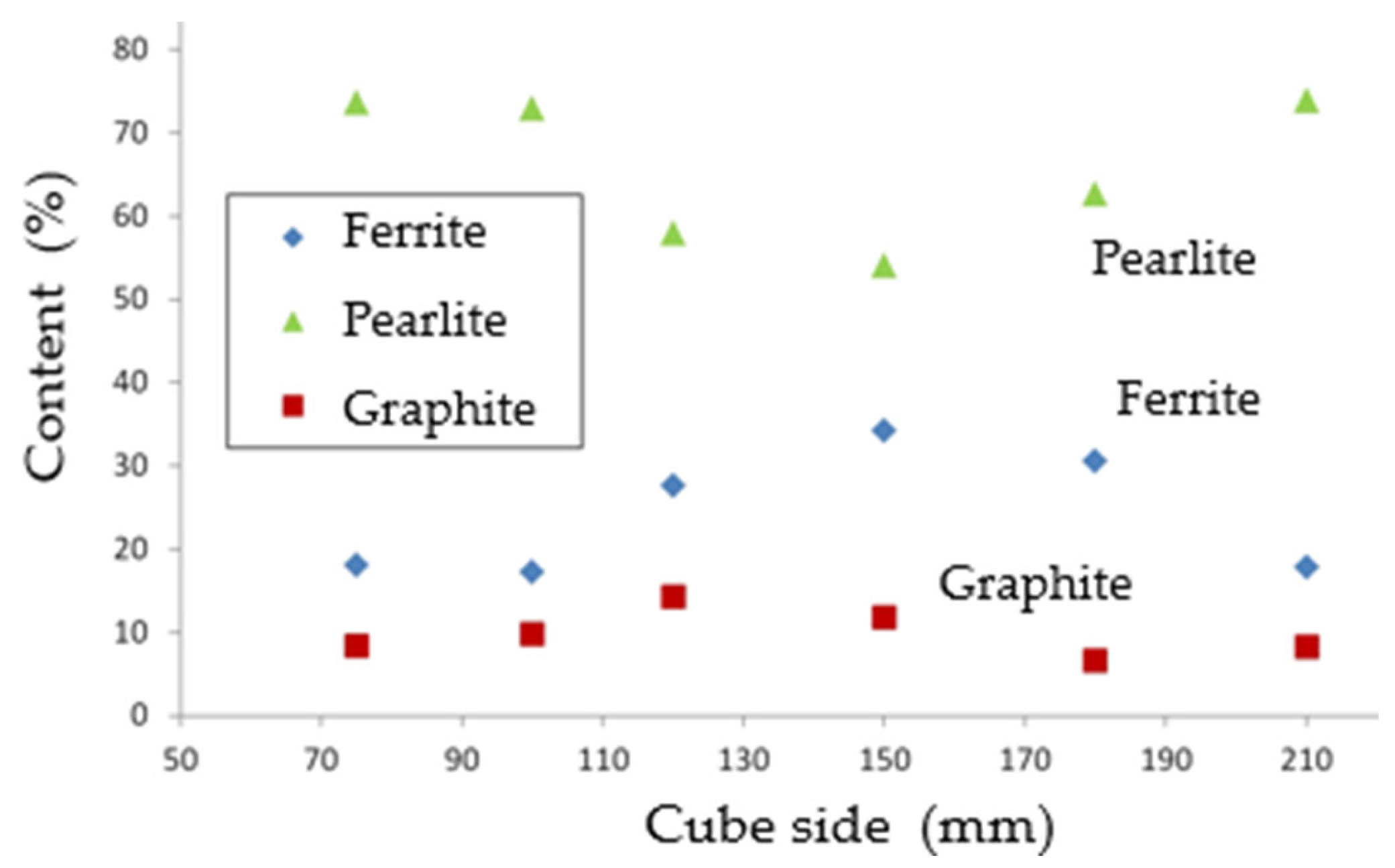
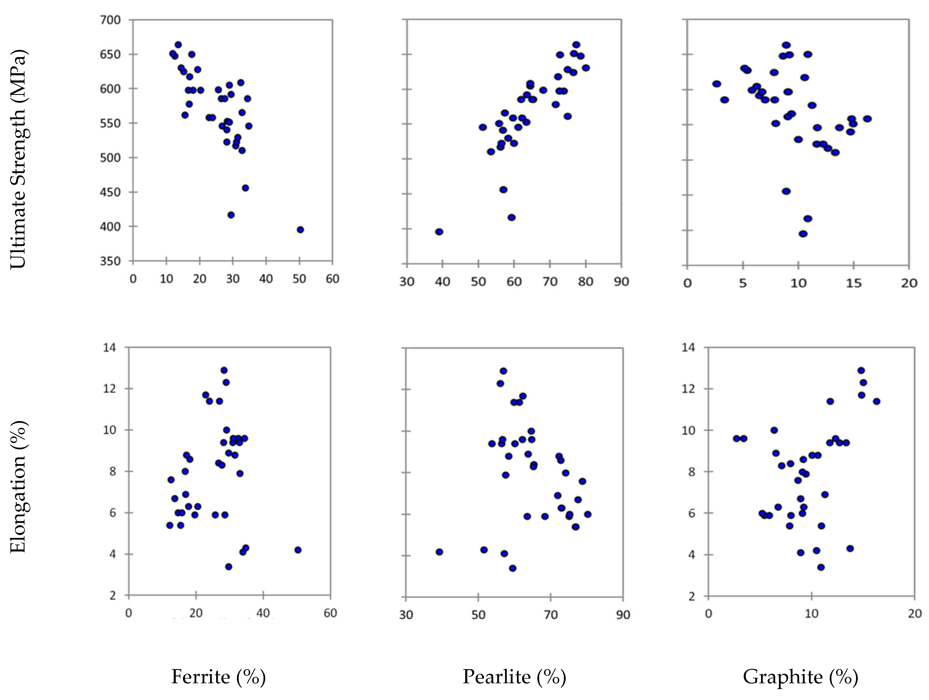
The present work prefers to focus its analysis on standardized factors, such as the contents of graphite (GR), ferrite (FE) and pearlite (PE), or the grade of nodularity (NO), considering their immediate correspondence with the physical meanings. For instance, we can observe that:
  • Graphite nodules in a completely ferritic matrix provide the cast iron with a good ductility, impact resistance, tensile strength (UTS) and yield strength (YS), making the cast iron almost equivalent to a non-alloy steel.
  • An almost completely pearlitic matrix, with small amounts of ferrite around the graphite nodules, gives the cast iron a high tensile strength, good wear resistance and moderate ductility, with a higher machinability than steel.
  • A mixed matrix consisting of ferrite and pearlite, the most frequent form of SGI as it appears in a foundry, gives the cast iron intermediate properties between the ferritic and pearlitic ones, with a good machinability and low production costs.
Returning to data mining applications for SGI, in [21], the k-nearest neighbors (kNN) learner, another supervised classifier, was used to predict defects in a foundry by relating historical process data (about the mold sand, pouring process, chemical composition, etc.) to the percentage of defective castings. This is a valid example regarding the use of ML for monitoring the quality of the casting process in the case of SGI, but it required a large amount of data in order to define the time series from which one can recognize the time-depending patterns. Thus, the present work is very different in terms of its data consistency and scope.
In [22], machine learning and pattern recognition were used to investigate an important aspect of the casting process: the cooling and solidification of the metal. In general, this aspect is also relevant in the present case, but the two investigations are based on different databases (i.e., mechanical properties vs. thermal analysis cooling curves).
Nevertheless, the use of artificial intelligence (AI) and data mining to investigate the materials’ behavior is a topic of great interest in current research. This is why a great number of articles deals with this theme. Limiting the discussion to the most recent contributions, in [23,24], ML methods were used to relate material defects (such as porosity), which emerged after solidification, with mechanical properties (such as fatigue strength). In other research papers, the use of ML tools was implemented in the earlier stages of the production process, with the aim of predicting impurities [25] or tracing the evolution of other chemical elements [26] inside the blast furnace hot metal. The general aim was to improve the level of control over the whole metal melting production process [27], which is characterized by a strong intrinsic variability. There are also interesting cases where an ML approach permitted the improvement of specifical material characteristics (such as the required impact strength in the case of [28]) or even the development of a substantially new and different cast alloy ([29]).
All these works, together with many similar studies (such as [30,31]), are mainly based on the validated assumption that ML can be conveniently applied for the recognition of the metal alloy microstructures, constituents, and morphological characteristics.
Nevertheless, even more relevant studies are those related to the prediction of mechanical properties in the case of cast irons, starting with their metallurgy characteristics. Firstly, it is interesting to mention [32], where ML algorithms properly classified nodular cast irons, while this ability was used to predict (by regression) the stress–strain [33], Poisson’s ratio [34] and hardness [35], even when comparing different ductile cast alloys [36].
However, unlike other studies, here an additional target is involved in the assessment of the proposed methods and tools with respect to a real industrial production environment.
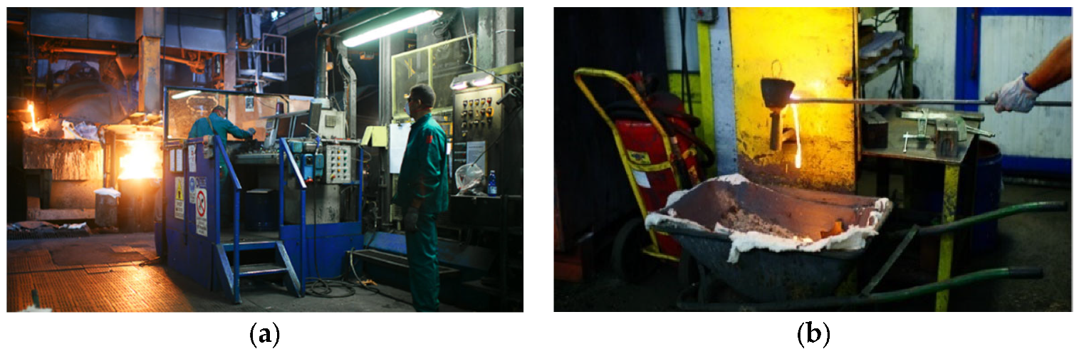
With such a scope, this research was designed to be implemented within a traditional sand cast iron foundry during its daily operation and without significant alterations to the process scheduling. Precise limits emerged from this work in terms of:
  • Production (e.g., alloys, geometries, process factors and specimen numbers);
  • Experiments (e.g., mechanical and microstructural tests);
  • Data mining (e.g., platforms, algorithms and data representation).
Finally, the research was intentionally based on methods that have already been applied in past, which, here, are largely reconsidered with the aim of providing additional outcomes.
Specifically, the abovementioned [10,11,12] offer similar experimental characterizations (tensile, flexural and fracture properties, respectively) of different cast irons, including SGI, produced using relatively analogous process conditions (i.e., open-cast conditions in green sand). Their measurements are very useful and, here, are used for the purposes of comparison and discussion.
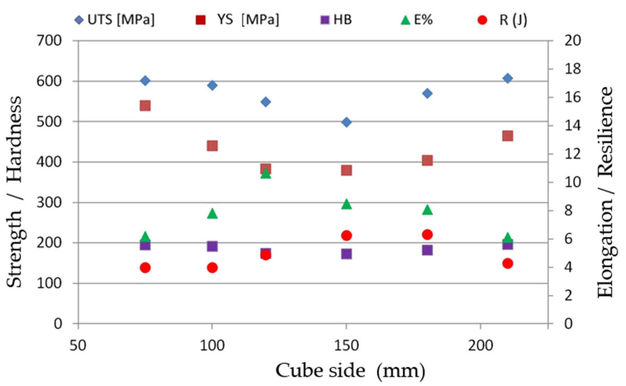
At the same time, these past investigations differ in the (smaller) number of specimens used and the means by which these specimens were produced. Here, for the first time, specimens were extracted from castings with the detection of their geometry, dimensions and processes, which are fully in line with those representing the daily production. These differences are important. For instance, while the characteristic dimension was defined as 26 mm in all the previous works, here, it varies from 75 to 220 mm, permitting a better investigation of the cooling phenomena.
Regarding methods, [35,37] offer a valid overview of the data mining techniques, which have been validated in the past and are used again here. Nevertheless, here, several important methodological improvements were combined so as to provide a fruitful analysis, including the following:
  • The dataset was enlarged by two additional features, including hardness and resilience.
  • The SVM was included in the ML procedure in light of the consistent results that other researchers achieved using this learner for their predictions.
  • Learners were optimized through changes to their constitutive parameters (vs. the default values used in the past), in accordance with their specific meanings.
  • The validation was performed on a different basis, improving the accuracy.

2. Materials and Methods

2.1. Casting Process

Specimens were manufactured using a traditional process of green sand molding in a hot-blast long-campaign cupola furnace [38]. Above the iron melting temperature (i.e., ~1250 °C in this case), the solid pieces of metal, alternated with hot coke in the furnace, were transformed into molten iron. Then, the molten metal was poured into an intermediate furnace, where the temperature, chemical composition and Mg contents (added by Fe-Si-Mg inoculation) were strictly controlled with the aim of establishing the suitable environment for the production of SGI. Then, the molten metal was transported using a ladle to the place of pouring and poured into sand molds, in which the iron was allowed to cool and solidify. A thermocouple was used to record representative cooling and solidification curves, without highlighting criticalities. Finally, the castings were shaped through tool machining to extract specimens with a (‘dog-bone’) geometry in accordance with the abovementioned standards.
Figure 1a offers a visual perspective of the foundry environment during the casting phases, showing the molten metal descending under the influence of gravity along the casting channels from the cupola (not visible, on the back) towards the secondary furnace, and from there falling into the ladle, while the operator activates the casting controls. Figure 1b highlights the phase of manual pouring of the fluid into the chemical analysis device.
The chemical composition (as the % of the weight) of the cast iron is reported in Table 1. It is representative of a conventional SGI (i.e., C, 3.3 ÷ 3.8%; Si, 1.8 ÷ 2.8%; Mn, ≤0.6%; P, ≤0.1%; S, ≤0.03%; Mg 0.04 ÷ 0.08%), apart from its slightly higher content of desferoidizers (e.g., Pb).
The mentioned processing phases represent a traditional casting process and similar experiments (e.g., [35,37]) but also include an important difference: the process was intended to offer the scope for analyzing different cooling conditions.
Within this scope, a single large sand mold was designed with several cubic chambers of different sizes, connected together as a “cluster of cubes” (Figure 2a). This expedient allowed all chambers to be poured almost simultaneously in a single casting stage, ensuring the same physicochemical characteristics of the melt. In Figure 2b, the various cubes (i.e., 50, 75, 100, 120, 150, 180, 210 mm) formed by ProCAST (ESI Group, Paris, France) are visible when separated, with indications of the subsequent cuts to be performed in order to obtain the “slices” from which the specimens can finally be extracted.

2.2. Mechanical Properties

A total of 36 specimens were extracted from the cubes and used to perform the tensile tests (an additional 36 and 14 specimens were produced for, respectively, the impact and fatigue tests, but these are not considered here). Depending on the cubes’ size (side) and local porosity, they were extracted from 1 to 3 specimens from each “slice”. In Figure 3a, for instance, we can observe the division of a 120 × 120 mm slice into 4 specimens and the selection of 3 of them.
In total, 9 specimens were derived from cubes of 210 and 180 mm, 6 from those of 150 and 120 mm and, finally, 3 from cubes of 100 and 75 mm. No specimen was extracted from the cube of 50 mm, as the dimensions would not have allowed for its proper analysis. These specimens, machined in the form of a ‘dog bone’ (Figure 3b), as defined by the standards, had variable diameters of 8, 11 and 13.5 mm depending on the cubes’ size (Figure 3c).
Tensile tests, according to ASTM E8/E8M-16, were carried out, providing the ultimate tensile strength (UTS in MPa), yield strength (YS in MPa) and ultimate strain/ductility (ε in %). The failure of all the specimens near the centerline confirmed the correct alignment and functionality of the gripping system (Figure 3c).
Resilience tests, according to ASTM A327M, were carried out, and the specimens used for these tests were extracted from an area close to the extraction area of the tensile specimens. Thus, their number was the same, being equal to 36. A micrograph was preliminarily created for the specimens to verify their status. Then, tests were carried out using the instrumented Charpy pendulum.
The Brinell hardness, according to ASTM E10-08, was also quantified. Measurements were directly performed on the tensile specimens to yield the average hardness detected in ≥6 different spots per specimen with a 2.5 mm diameter sphere and 62.5 kg load.

2.3. Metallographic Analysis

Other specimens were obtained with the aim of implementing a metallographic analysis. Special attention was given to ensuring the good condition of the surfaces. Brazing papers (with a grain size between 200 and 1000 grit), soft cloths and a lapping machine (Struers LaboPol_5®, Ballerup, Denmark, with a 10–15 N load and 150 rpm rotation speed) were used for the smoothing and polishing. These specimens were also subjected to a chemical attack (with “Nital2” reagent for 10 s) with the aim of highlighting the microstructure of the matrix. For each specimen, 9 micrographs were acquired both before and after the chemical attack, with a total analyzed area of 40 mm2, being well distributed over the overall surface. In this way, it was possible to identify the micrograph values by characterizing the whole specimen.
Two micrographs are visible in Figure 4. A 58× magnitude shows an intense nodular area identified on a cube with a side length of 120 mm (Figure 4a), and a 2000× enlargement highlights the details of a spheroidal nodule of the graphite (Figure 4b).
The micrographs were processed using image analysis software (Image-Pro® by Media Cybernetics, Rockville, MD, USA), thus providing the average values of the graphitic (GR), ferritic (FE) and pearlitic (PE) fraction, the number and size of the graphite nodules, and, finally, the nodularity (NO) for each specimen.

3. Results

3.1. Experimental Measurements

Figure 5 shows the content of ferrite, pearlite and graphite in each specimen. Figure 6 displays the values of the tensile strength (UTS), yield strength (YS), elongation at break (ε), hardness (HB) and resilience (R) for each specimen.
These values are also reported in Table A1 of Appendix A, together their means (μ), standard deviations (σ) and relative standard deviations (σ%).
At first glance, it is evident that:
  • The cast iron has a pearlitic-ferritic matrix with an average presence of about 65% pearlite and with an average nodularity that is also of the order of 65%.
  • The cast iron, also due to its predominantly pearlitic matrix, has a rather low resilience (at room temperature).
  • The extreme variability in the microstructure, with differences of up to 34% (in terms of σ%) in the main parameters, suggests significant variations in the mechanical properties.
The same data can also be grouped according to the representative size of the casting from which the specimens were extracted (cube side), as in Figure 7 and Figure 8, and/or investigated in terms of the relationships between the material characteristics (both mechanical and microstructural), as in Figure 9, Figure 10 and Figure 11. Considering these trends, some aspects seem to be evident, and others less so. For instance, the increase in the ferrite and the decrease in perlite as the size of the cube increases can easily be associated with the increase in the cooling time required. At this point, however, the trend reversal after 150 mm becomes less clear, indicating that the phenomena under investigation may lose linearity over the range of interest.

3.2. Trend Analysis

Considering the data trends (as shown in diagrams), it was possible to observe that:
  • The ferrite content decreases with the increasing cube side, with a peak in correspondence with the cube side at around 150 mm, then starts to increase more slowly (Figure 7).
  • The pearlite content behaves in the opposite manner (with respect to the ferrite), increasing with the cube side, with a peak in correspondence with cube side at around 150 mm, again, before starting to decrease more slowly (Figure 7).
  • The graphite content shows no significant trends, remaining approximately constant as the size of the cube varies (Figure 7).
  • There is an incremental trend in the number of nodules as the cube side decreases, without, however, a corresponding variation in the size of the nodules (Figure 9).
  • At high solidification/cooling rates (i.e., small cubes), many graphite nuclei are present, but a very limited time is required for the diffusion of the carbon from the austenite to the nodules and, therefore, there is an increase in their size. This corresponds to the high presence of pearlite (Figure 9).
  • For large cubes, on the other hand, the low solidification/cooling rates lead to the formation of a reduced number of graphite nuclei, which are more distant from each other and, therefore, despite the greater time available for the carbon diffusion, these cannot grow beyond certain dimensions. This situation also favors the formation of pearlite (Figure 9).
  • With respect to cubes of intermediate sizes, it seems that they correspond conditions that favor the formation of ferrite.
  • As the cube side decreases, the number of nodules observed per unit of surface area increases. The nodularity also increases with the decreasing size, while a monotonous trend could not be observed as regards the size of the nuclei (Figure 9).
  • With the increase in the UTS, YS and HB, a decrease in R and ε is observed (Figure 8). It is certainly not by chance that these variations follow a non-linear trend similar to that observed for the structural constituents of the matrices (Figure 10).
  • In accordance with the literature, the increase (decrease) in the ferritic phase in favor of the pearlitic one is accompanied by a decrease (increase) in the tensile properties and hardness and an increase (decrease) in the ductility and toughness (Figure 10).
  • The graphitic fraction does not appear to be systematically linked to any of the properties. However, it appears that its increase corresponds to a non-marginal tendency towards a decrease in the hardness, tensile strength and yield strength (Figure 10).
  • It can generally be confirmed that there is a remarkable correlation between the microstructure and tensile strength/elongation (Figure 10).
  • It can be also confirmed that the hardness is a significant parameter for defining the mechanical behavior of spheroidal cast iron, as indicated by the trend in the UTS, YS and ε as a function of HB (Figure 11).

4. Data Mining Perspective

4.1. Dataset and Datatool

From a data mining perspective, the dataset consists of 36 instances (i.e., the numerical vector collecting data from each specimen) and 12 features (i.e., each measured characteristic), equivalent to 432 data. No value is missing (e.g., measurements that are not made or are incorrect), and all data are numeric (i.e., no categorical or time-series data).
The data analysis was performed using the Orange Data Mining platform [39]. This is an effective and efficient open-source toolbox developed by the University of Ljubljana for data analysis and visualization. It enables the relatively easy use of supervised and unsupervised machine learning (ML) tools and their built-in learners/solvers [40].
Specifically, a workflow was arranged within the scope of the study through the visual programming enabled by the platform and by using widgets and links (as exemplified in Figure 12).
The data analysis can only begin after the identification of the target. Essentially, one feature has to be selected as the target. In this case, the cube side was set as the (initial) target, with the aim of investigating (firstly) the influence of the geometric features on the microstructural characteristics (e.g., ferrite, graphite, etc.) and, consequently, on the mechanical properties of the cast iron (e.g., UTS, YS, etc.). (Later, the analysis was extended to include all features as targets.)

4.2. Principal Component Analysis

The principal component analysis (PCA), however, confirmed that the features are not fully independent. Specifically, 4 principal components (instead of 11 features), should be enough to recreate the dataset with an accuracy of ~90%. With 8 principal components, the accuracy is established as ~99.2%, while the 10th and 11th principal components are useless (Table 2).

4.3. Correlation Analysis

Through a correlation analysis (CA), performed using Pearson (rpxy) or Spearman (rsxy) coefficients, it is possible to quantify the relations [41,42]. For example, by referring to the dimension of the cubes (side), the Pearson coefficient highlights its inverse linear correlation with the nodularity (rpxy = −0.744), nodular density (rpxy = −0.624) and graphite content (rpxy = −0.420). This means that the dimension of the castings reduces the nodularity almost proportionally, affecting the nodular density (but not the nodules’ dimensions) and, to a lesser extent, the graphite content.
Such correlations can be (slightly) improved when a Spearman coefficient is used (with rsxy = −0,766, −0.707 and −0.469, respectively). While Pearson’s correlation assesses linear relationships, Spearman’s correlation assesses monotonic relationships, whether they are linear or not. Other variables are not significatively influenced by the dimension of the cubes (side).
The CA can be extended to all parameters, allowing other correlations to emerge. Some of these are evident (e.g., ferrite vs. pearlite, rsxy = −0.935) or already discussed (e.g., the nodule density vs. cube size, rsxy = −0.624), while other are less evident. They are more interesting when related by Spearman’s correlation coefficient which, as mentioned, goes beyond linear relationships. Table 3 reports the top ten highest correlations.
For instance, the table indicates that the resilience (R) is deeply dependent on the alloy contents of pearlite (i.e., it is proportionate) and ferrite (i.e., it is inversely proportionate). The R is also significantly correlated with the other material properties, such as the UTS and YS. Even if these concepts already emerged during the data discussion, here, a specific indicator (i.e., Pearson or Spearman’s coefficients) confirms the accuracy of the data interpretation, also providing a clear measurement/weight of the relationship.

4.4. Rank Analysis

Through rank analysis, it is possible to score variables according to their relevance with respect to the target variable. The method is based on scorers. In the present case, characterized by the regression of the numerical data, the in-built scoring methods are:
  • Univariate regression: linear regression for a single variable.
  • RReliefF: relative distance between the predicted (class) values of two instances.
According to the univariate regression, for instance, the UTS is influenced (in order) by the pearlite (score = 73), ferrite (45) and nodular density (21), and much less by the graphite (6). Similarly, the YS, too, is shown to be influenced by the pearlite, ferrite and graphite, but not by the nodular density (score = 1). This is an interesting difference.
Using a rank analysis, it is also easy to quickly identify and quantify relationships between variables (here, features). It is possible to include additional ranking methods, such as PCA or CA, but ML learners also offer a very powerful tool.

4.5. Machine Learning

The ML methods discussed here are based on training and use supervised learners. Specifically, the following learners were preferred for this study (in alphabetical order):
  • Classification tree               (CT)
  • k-nearest neighbors            (kNN)
  • Neural network                   (NN)
  • Random forest                     (RF)
  • Support vector machine     (SVM)
For the theory behind these mathematical tools, the reader should refer to specialized texts. For their validation and practical use in similar cases, the reader can refer to [43].
Specifically, according to common practice for the use and validation of ML algorithms, the dataset was fractionized into two parts, one for training and the other for testing the learners’ ability to make predictions. Random sampling randomly splits the data into the training and testing sets in the given proportions. Then, the whole procedure is repeated a specified number of times. Here, different settings were considered, with the most balanced results achieved using 90% of the data for the training and 10% for the testing. In practice, respectively, 32 and 4 of the 36 available items were used, with 10–20 repetitions so as to statistically consolidate the results. Then, the learners’ degrees of effectiveness were compared and ranked.
For performance statistics, several standard methods may be used (e.g., mean square error, relative mean square error, mean absolute error, etc.). In the present discussion, the coefficient of determination (R2) was preferred due to its relationship with the Pearson correlation coefficient and its linearity. The R2 is interpreted as the proportion of the variance in the dependent variable that is predicted using the independent variable. In brief, the R2 can be between −∞ and 1. When R2 = 0, this means that the adopted model offers an interpretation of that data that is not better than the average data value and, under 0, the model is even worse than the average value. However, when R2 = 1, this means that the model perfectly explains the data.
The initial tests, which used the default settings for the learners, were not especially encouraging, with the R2 often being negative and never higher than + 0.3/0.4. However, after some changes to the settings, the accuracies were greatly improved, especially for NN and RF, with an R2 over 0.9. This means that these learners are extremely precise in predicting the target values. SVM and tree also offer a reasonable level of accuracy. In the case of SVM, which is frequently used in similar investigations on cast irons, a precision level of 82–85% was also confirmed here.
The following (main) parameters were selected in order to achieve the declared accuracy:
  • NN: max 500 neurons in hidden layers, logistic activation, L-BFGS-B solver, max 400 iterations, and regularization at 0.0001
  • RF: max 24 trees, 5 attributes at each split, and 3 as the limit depth of individual trees.
  • SVM: cost = 200, regression loss epsilon = 1.00, and kernel polynomial.
  • Tree: max 7 instances in the leaves, 3 as the smaller subset, and 10 as the max tree depth, stopping when the majority reaches 99%.
  • kNN: five as the number of neighbors, Mahalanobis metrics, and uniform weight.
Table 4 offers an a priori evaluation of the learners using all the available methods.

4.6. Predictions

After the learners’ validation, they were used to predict the target values (Table A2 in Appendix A). Specifically, the ‘leave on out’ approach was applied. This means that one specimen was excluded from the dataset, and the others (35) were used to train the learners. Then, they were required to predict the target value in the case of the excluded specimen. The same process was repeated for each specimen, with the aim of predicting every available target value. In other words, the learners were required to offer their best evaluation of the cube side for each specimen, considering all the others. The results are shown in 
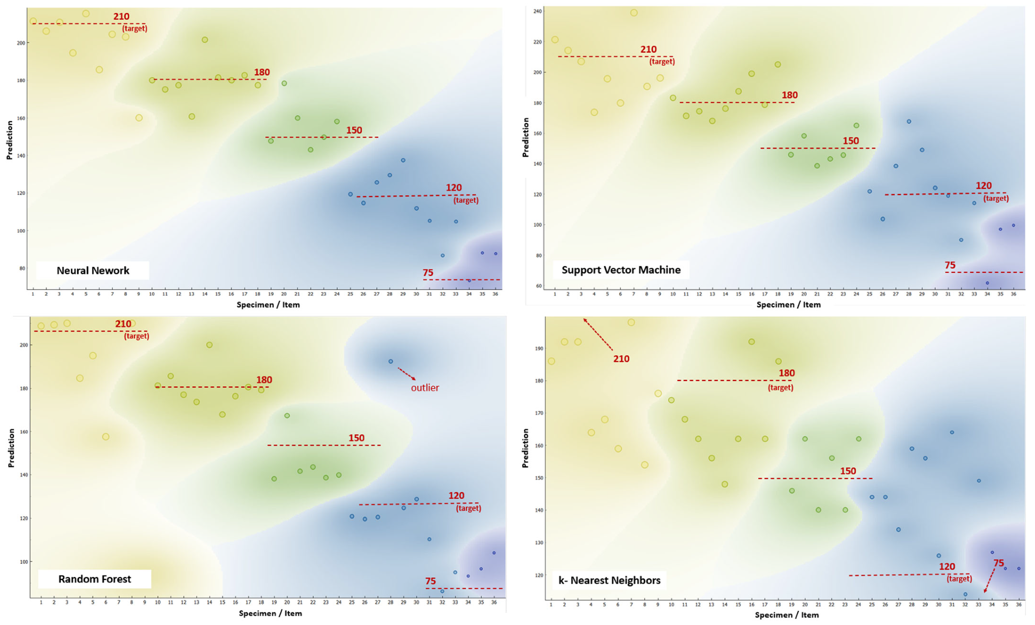
Figure 13 in terms of the predicted and expected target values. The accuracy is evident.
Specifically, the accuracy offered by NN, SVM, RF and k-NN was evaluated by measuring the correlations between the predicted and expected values using Pearson’s coefficient, which equaled, respectively, rpxy = 0.952, 0.914, 0,799 and 0.768. The tree classification is ignored here, since its results were always in line with those of RF (e.g., rpxy = 0.746).
Details regarding the full correlation analysis are available in Table 5.
With respect to the initial comparison of the learners (performed a priori using a different method, the R2), the high accuracy rate of NN is also confirmed here. As evident in the diagram, the NN learner is able to categorize predictions for the five target values (210, 180, 150, 120, 75). The overlap between categories is quite limited, and no evident outliers exist, as in the case of RF. SVM’s accuracy is also confirmed. Indeed, for this different classification, performed a posteriori, it is better than RF, confirming the validity of other researchers’ decision to use SVM for their own analyses. The difference in precision between NN and SVM is minimal and mainly linked to the data variability with respect to one of the categories (target = 120), which appears to be the most complex class recognized here, possibly due to a stronger variability among the input data. An inadequate precision is instead evident in the graph of k-NN. The learner tends not to categorize values into groups but into indifferent ones within the same range (e.g., 130–180). This creates several problems, such as, e.g., an inability to identify all the targets and loss of the extremes (i.e., 75 and 210).
The learners’ levels of precision can be represented using a diagram of the predicted vs. expected values (as in Figure 14, in the representative cases of NN and k-NN), where the points closer to the bisector line represent the highest prediction accuracy, and their distance from that line exemplifies the error. It is evident that NN, in comparison with k-NN, exhibits points more clustered points around the bisector line.

5. Discussion

5.1. Preliminary Considerations

The analysis of material experimental data is a complex task, especially in the presence (as in this case) of intrinsic variability in the process conditions and material properties, which are closely related to each other. Nevertheless, with adequate attention and expertise, it is possible to reconstruct the physical meaning of the experimental data, resulting in a myriad of new information and considerations (as discussed in Section 3.2).
In light of so many important new ‘outcomes’, one might consider that the data analysis could not be achieved. In this case, however, the additional benefits offered by the advanced application of a data mining procedure would be lost.
In general, it is plausible to state that a data mining process, based on an ML methodology, permits researchers to (precisely):
  • Recognize and analyze non-linear effects.
  • Measure and quantify outcomes.
  • Predict phenomena and their probability of occurrence.
  • These concepts deserve a better explanation.

5.2. Recognizability

In experimental data analysis, less clear-cut results stem from non-linear relationships, which are very difficult to observe without using a data mining approach. Non-linearity can occur, for instance, when the variable under investigation is related to:
  • One variable (or more), but not linearly.
  • Two (or more) variables, even if they are linearly related.
This occurred frequently with our data. In this regard, the PCA highlighted two patterns that were not independent (when the data matrix was rearranged with respect to a linearly independent vector base, although, from a physical point of view, this is of little interest for this specific case).

5.3. Quantifiability

In experimental data analysis, data-driven considerations are often provided without their real quantification. For example, from Figure 7, it is evident that there is a ferrite/pearlite inverse trend with respect to the cube side. However, this graph groups measurements around specific cube sides (e.g., 75, 100, etc.), and in any case, their numbers are very different (3 ÷ 9). Thus, a quantification is convenient. The Spearman correlation (rsxy = −0.878), applied to the draft data (Figure 5), confirms that a monotonous relationship exists, while the Pearson correlation (rpxy = −0.935~−1) indicates that this relationship is strong and linear (not just monotonous). Their negative values finally prove the inverse trend.
Similarly, Table 6 reports an overview of the scoring of the Pearson and Spearmen coefficients, respectively, showing the linear and monotonic relationships between variables. Many of the concepts discussed in Section 3.2 plainly emerge here. For instance, the great positive influence of pearlite on three of the five mechanical properties can immediately be noted (R, UTS and Y, with very high correlations). At the same time, the scores also highlight that pearlite moderately influences the hardness (HB) and has marginal effects on the elongation/ductility (ε).
However, the concept expressed here aims to be more general. Statistics tools (with the Pearson and Spearman correlations only representing two out of many) can be integrated naturally into a data mining approach, with the aim of measuring and ranking (obvious and less obvious) relationships. To achieve this aim, ranking tools are available and permit us to classify relationships according to a large range of classifiers.

5.4. Predictability

An accurate predictability of the phenomena represents the highest level of compression in science. In this specific case, five AI algorithms were trained, which were used for the prediction and compared, showing a very high accuracy of up to 95% (Table 5, NN learner).
This means that, with 11 parameters being known, it was possible to estimate the 12th with a high degree of precision. Such a result was obtained with respect to a specific target feature (i.e., the cube side). This implies, e.g., that when the microstructure and mechanical properties of a specimen are known, it is possible to recognize the dimensions of the cube from which it originated.
However, nothing prevents us from repeating the analyses with respect to another target.
It is conceptually possible to estimate any of the mechanical properties, thus avoiding the performance of a test. For example, we can ask the system to identify the expected resilience or the expected hardness knowing all the other (microstructural and mechanical) values.
It is also possible to estimate the value of such a target property (e.g., the hardness) as a function of another one (e.g., the resilience) when knowing the others. The resulting ‘isocurves’ can be used to support the development of new alloys or process monitoring.
This approach constitutes a first step toward the solution of an ‘inverse problem’ that has always been crucial for casting processes and foundries: the question of how to derive the cast iron microstructure from the expected/desired mechanical characteristics.
An AI system, based on machine learning, can help to find the solution through, e.g., a ‘pattern recognition’ approach applied to the myriads of date used for the training. These data, as demonstrated in Table 6, emerge from a multitude of relationships, which may be strong or weak, direct or inverse, linear or non-linear, and so on. In this case, an automated recognition of the patterns and regularities in the data can ‘unravel the skein’.
In this study, the analysis was repeated 11 additional times, considering each of the features as the new target variable and comparing results. As implemented before, 90% of the available data were used for the training and the residual 10% for the validation/comparison, replicating the process 20 times so as to ensure the statistical significance of the results.
Here, the analysis was limited to the NN, RF and SVM learners, and their comparison was performed (again) using the coefficient of determination (R2), since this parameter can be more (intuitively) informative. The results (Table 7) show:
  • A high accuracy rate of the predictions, especially evident in the case of the microstructural properties.
  • The graphite, ferrite and pearlite contents are fully predictable.
  • The nodular area and density are also predictable with a low margin of error.
  • The estimation of the nodularity is less accurate but still of an acceptable level.
  • The casting dimension affects these properties in a very predictable way.
  • The NN learner shows the highest accuracy, but other learners have a good usability.
  • The prediction of the mechanical properties represents a more complex task.
  • The UTS and R are acceptably predictable (R2~0.75), but improvements are required.
  • NN does is not especially useful; the other learners work better.

5.5. Learners

It is not possible, unfortunately, to identify the most suitable ML learner with respect to a given dataset in advance [44,45,46,47]; a testing and scoring procedure is always required. Similarly, it is also useful to carefully modulate the leaners’ settings (i.e., the so-called hyperparameters).

5.5.1. Neural Network

  • NN (as implemented in Orange) is a very powerful method, as long as due attention is given to the correct choice of the activation (identity, logistic, tanh, Relu) and solver (i.e., L-BFGS-B, SDM, Adam).
  • Relu activation, which is quite common and the first historically implemented method, due to its simplicity, does not offer impressive results (compared to identity and logistic).
  • The L-BFGS-B solver is stable in its predictions, offering excellent results when predicting microstructures, while only Adam manages to come close to the prediction of the mechanical properties (which, however, is almost always inadequate).
  • Of course, the number of hidden neurons in the network affect the results, but not excessively so. The problem under investigation, in this sense, is not highly complex and, above the level of 60–80 hidden neurons, the accuracy of the prediction increases slowly up to around 200/300. Beyond this second threshold, no improvements are evident.

5.5.2. Random Forest

  • RF is a classifier based on a ‘forest’ of classification trees, which is very sensitive to the number of trees and their replication speed. At the level of over 10–15 trees, the accuracy is stable.
  • RF is not able to offer outstanding results in any case but, on the other hand, it is stable with respect to the learner settings (e.g., attributes considered in each split, the depth of individual trees, etc.). This represents a great advantage in its practical use.
  • Here, RF provided better predictions than tree. This was expected, since RF represents a methodological extension of this learner, using multiple independent decision trees. At the same time, RF’s superiority was often limited, demonstrating that the complex data could be also managed by a single decision tree.

5.5.3. Support Vector Machine

  • SVM has been confirmed as a powerful and flexible learner, which is able to offer valid predictions in the material data analysis.
  • Its flexibility is based on its constant parameters (e.g., cost, regression loss epsilon, etc.), which can (be made to) assume a wide range of values (from 0.1 to 400, here), with significant impacts on the predictions.
  • SVM is also highly subject to the kernel type, whereas linear and polynomial (instead of RBF and sigmoid) were the best in terms of accuracy.

5.6. Analysis with Respect to the State-of-the-Art Literature

Even if, as shown by the literature review, there are few scientific papers on this specific subject (i.e., the use of machine learning to identify relationships between the microstructure and strength properties in the case of nodular cast iron), the results are in line with the available state-of-the-art literature. For instance, [48,49] used an identical approach, based on information about the chemical composition, process variables (i.e., temperature) and microstructure, to predict the tensile strength of steels. In particular, in [49], an NN with 20 variables was applied, achieving a comparable accuracy (i.e., 93% in terms of the R2 coefficient) in the prediction of the yield (YS) and ultimate (UTS) strength.
In general, two ML methods have been favored by researchers, these being NN and SVM [27,32,33,35], which also offered the best accuracy here (Table 5). As regards NN, the ability to predict the material properties was rather as expected, but this was not the case for SVM. As a method that defines a hyperplane in order to separate data belonging to two classes with a maximum margin, this method seemed to be more suitable for classification problems than for regression (as the present paper has shown). Such considerations (about learners) were also confirmed in [37], where a general assessment of the ability of machine learning methods to predict the mechanical parameters of castings using a different approach to the image analysis was reported.

5.7. Improvements

Apart from the learners, a better prediction accuracy can be also achieved by the following considerations.

5.7.1. Dataset Enhancement

Using new experiments and data, the dataset can be enlarged (in quantity) and improved (in quality). It is well known that ML tools are more useful and powerful when more data is available. At the same time, more data can cause the pattern recognition to be more complex when non-homogeneous information is also introduced. This is why even rather small datasets (such as the one used here), especially if they are very homogeneous, can assure accurate predictions.
A comparative test was carried out by including the experimental data from [35,37] in the dataset, consisting of 27 instances in addition to the current 36 (+75%). However, they are defined by 8 features (instead of 12), including the casting dimension (side), which is a fixed value (=25 mm). Specifically, the following categories are missing: area, ρ, HB and R, where, based on the results already described, area and ρ should not be essential, as they can be derived from the other metallographic properties. Thus, the complex dataset contained 756 (63 × 12) data with 108 (27 × 4) missing values, being equal to 14%. To avoid these missing values, dataset was downscaled to 504 (63 × 8), which is equivalent to + 16% with respect to the initial set (this was achieved, however, by reducing the number of features’).
With respect to this new enhanced dataset, the analysis was duplicated to estimate the mechanical properties (i.e., the microstructural properties were already predicted with an extreme level of precision). Specifically, in the cases of the UTS (0.912, kNN) and YS (0.886, RF), the accuracy of the predictions was through the introduction of new data. The opposite case was observed for the elongation (ε); no learner was able to offer proper modelling.

5.7.2. Dataset Pre-Processing

The pre-processing of available data is an important aspect of data mining, since incoherent information can hinder the solvers. Data pre-processing mainly consists of:
  • Filtering incoherent data (e.g., outliers, shown as red spots in Figure 11, the UTS diagrams).
  • The identification and elimination of ‘unnecessary’ features.
While outliers are commonly related to experimental errors or variability and should be addressed carefully, the presence of ‘unnecessary’ features represents an intrinsic aspect of the dataset that must be understood before the data analysis begins. Two opposite cases can occur:
  • A feature is not significant, directly or indirectly, for the object under study (target).
  • A feature is directly derivable from another feature.
In both cases, in practice, the dataset includes data that are useless for understanding relationships, while they are misleading when evaluating the accuracy. Pattern recognition works, in fact, through information, and not based on the amount of data.
The principal component analysis (PCA) was useful for understanding the situation, enabling the quantification of the number of independent variables that were present in the system, while the correlation analysis (CA) enabled the identification of variables that were linearly dependent in order to enable (eventually) the reduction of the dataset.
In the present case, the CA (Table 6) made it clear that no direct correlation exists (rpxy or rsxy = 1). The features are most linked by a weak (<0.50) or medium (<0.75) correlation. Only 10 relationships (out of 66), accounting for 15%, can be defined as strongly correlated.
Among these, only those already mentioned (FE vs. PE) and (PE vs. R) are significative (>0.90). As a result, there was no need to ‘downgrade’ the dataset in the present study. However, here, the operation was introduced simply in order to verify the effect. The FE and R features were deleted from the dataset, one after the other, with the effect, as expected, of producing no clear modification of the precision offered by NN.

6. Conclusions and Future Work

The present experimental investigation was focused on a nodular cast iron, a material that has found an increasing number of applications in industry over the last few decades. This alloy, like many others, has metallurgical and mechanical properties that are closely related to each other. Moreover, even minimal changes in the chemical composition and/or process parameters may significantly affect such properties. It follows that cast iron, including nodular cast iron, has been extensively studied, starting with experimental measurements, to develop predictive models.
Here, data mining and machine learning techniques were used to perform a data analysis in search of information that was not evident, rather than a more traditional method of study.
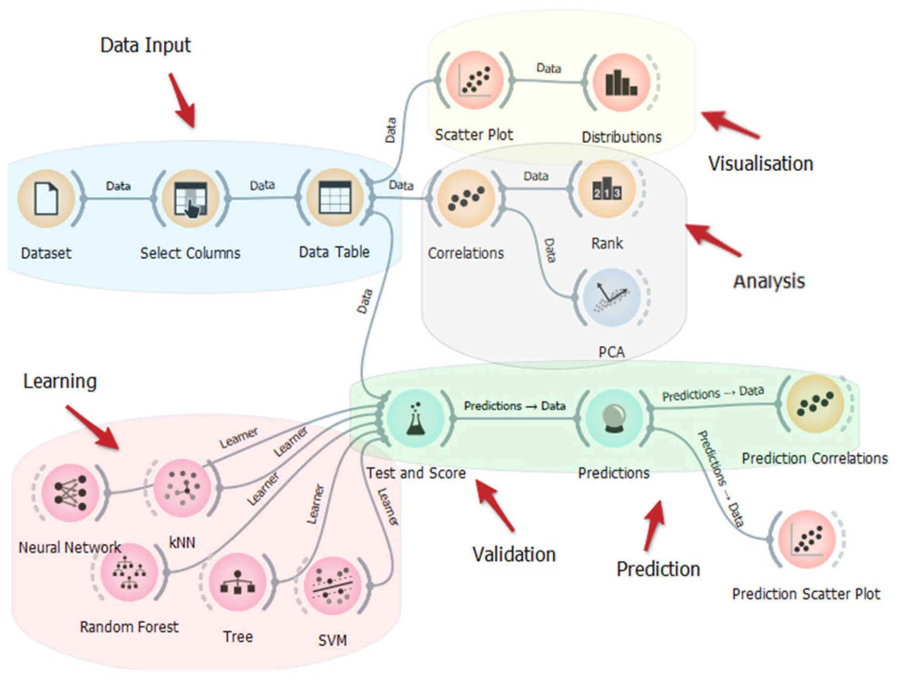
The experimental data were derived through an experiment designed to ensure adequate consistency with respect to some key aspects of casting (e.g., the characteristic dimensions) but also to the operation of a traditional foundry. The measurements were performed through standard tests: image analysis for the microstructures and strength tests for the mechanics. Firstly, considerations were developed through a preliminary data evaluation. Then, the dataset, consisting of 36 instances × 12 features, was analyzed by principal component analysis (PCA) and correlation analysis (CA), which permitted the identification and weighting of the correlations. Finally, data were used to train several different machine learning (ML) algorithms on the Orange Data Mining platform, including random forest (RF), neural network (NN), k-nearest neighbors (kNN) and the support vector machine (SVM), which are able to predict material properties with remarkable accuracy (i.e., >90% in half of the cases).
The next step in the research is to overcome the limits imposed by the current dataset, whose consistency varies from 432 to 756 values, which, through appropriate pre-processing, could be extended to even more than one thousand data. However, this number is still quite low for expressing the ML potential. At the same time, it must be considered that the prediction accuracy is more closely related to the data quality than the numerosity. Foundry processes are intrinsically variable, and every action aimed at expanding the dataset must take this into account. This means, e.g., that it is not convenient to merge data from other investigations if they are subject to dissimilar (processes and materials) conditions. However, a different approach can be taken, with the aim of extracting more data from the available information. Specifically, it is possible to integrate the current dataset with information from a different image analysis. Here, each microstructure was considered according to specific parameters (such as, e.g., the pearlite, nodularity, nodular area, etc.), as in many other similar studies. Later, this information could be integrated through the output of an image embedder that is capable of transforming the image into hundreds of new parameters (limiting the choice to the most significant ones in the PCA). Beyond this explosion of the data and parameters, however, we must understand whether new and useful information is really embedded in the analysis.
A second way of improving the method is the introduction of a diverse concept of supervised learning. Although some of the learners offered excellent predictions, they also proved to be quite erratic and unpredictable. One of the most recently tested ways of overcoming this (rather common) limitation combines the predictions in what is called ensemble learning. Among its different techniques, the stacking technique is expected to be more valid, which can be used to introduce an additional ‘meta-learner’ (usually a linear regression) that is trained using the predictions of those learners, which, here, were scored as the most effective through the cross-validation.

Funding

This research was co-funded by Region Emilia-Romagna and the European Regional Development Fund (ERDF) program.

Data Availability Statement

Consistent data are contained within the article.

Acknowledgments

The cast iron castings were formed at the SCM Foundry in Rimini (Italy). Experimental tests were performed at the CRIF Laboratory in Rimini (Italy). Special thanks go to Stefano Cucchetti and Giuseppe Lucisano for their support.

Conflicts of Interest

The author declares no conflict of interest.

Abbreviations

The following nomenclature was adopted
GJSSpheroidal graphite cast iron (EN 1563 denomination)
SGISpheroidal graphite cast iron (standard denomination)
SEMScanning electron microscope
SideCasting representative dimension [mm]
GRGraphite (grade of)[%]
FEFerrite (grade of)[%]
PEPearlite (grade of)[%]
NONodularity (grade of)[%]
AreaNodule area[μm2]
ρNodule density[N/mm−2]
UTSUltimate tensile strength[MPa]
YSYield strength[MPa]
εElongation at break/ultimate strain[%]
HBBrinell hardness[-]
RResilience[J]
AIArtificial intelligence
MLMachine learning
RFRandom forest learning algorithm
NNNeural network learning algorithm
kNNk-Nearest neighbors learning algorithm
SVMSupport vector machine learning algorithm
TreeClassification tree learning algorithm
PCAPrincipal component analysis
CACorrelation analysis
μMean value
σStandard deviation
σ%Relative standard deviation
rpxyPearson correlation coefficient
rsxySpearman correlation coefficient
R2Coefficient of determination
MSEMean square error
RMSERelative mean square error
MAEMean absolute error
CVRMSECoefficient of determination of RMSE

Appendix A

Table A1. Metallographic characteristics (graphite, ferrite and pearlite contents; nodularity; density; and area of graphite nodules) and mechanical properties of the spheroidal cast iron (yield strength (YS), tensile strength (UTS), elongation at break [ε], hardness (HB) and resilience (R)).
N.SideGraphiteFerritePearliteNodularityYSUTSεHBR
mm%%%%μm2N/mm−2MPaMPa%HB10J
12107.815.476.741.35287155206245.44196
22108.712.678.748.85527164556477.64.5197
32108.913.777.452.24761194876636.74.5197
42105.925.868.449.52199274555985.94196
521010.617.172.361.25009214876178.85202
621010.929.759.413.92217493904163.44177
72105.419.675.025.93346164556275.94198
82105.214.680.248.427821945563064199
921010.912.176.972.45527204876505.44.5206
101806.529.763.741.73805174225918.96.5183
111806.329.164.656.9383117435604105.5180
121808.028.563.564.43405233905525.97184
131809.433.057.557.32914323905657.96.5179
141807.926.865.358.83336243905858.45187
151808.933.957.234.42977303904554.18180
161803.434.562.129.41516223905859.65.5175
171807.127.865.252.83154224095858.36180
181802.732.664.730.01243224226089.67193
1915012.730.956.476.14354293955169.45.5167
2015010.550.439.143.32444433313954.27164
2115013.432.953.780.15044263825109.45177
2215012.331.156.690.04188293825229.67179
2315011.728.260.181.04453263955229.45.5173
2415010.131.658.385.53978253955298.87.5178
2512015.029.056.085.738543936455112.35171
2612014.822.962.284.745693239055811.74.5179
2712011.827.061.282.738793044254511.44.5179
2812013.734.851.568.14022343645454.34175
2912016.324.059.887.156812936455811.45175
3012014.828.356.988.139983737754012.95.5172
3110011.316.971.890.13935294165776.94195
321009.218.172.786.72863325195978.64192
331009.116.874.186.128503239059784190
34759.115.875.183.322764051956164194
35759.217.873.085.52636355586496.34196
36756.720.572.876.21555435455976.34195
μ9.625.465.02863.963.9285687.95185
σ3.38.39.2821.821.88612.41.210
σ%34%32%14%28%34%34%28%10%30%24%5%
Min.2.712.139.11513.913.9153953.44164
Max.16.350.480.24990.190.14966312.98206
Table A2. Target and predicted values by the neural network (NN), support vector machine (SVM), random forest (RF), classification tree (Tree), k-nearest neighbors (kNN) learning algorithms.
N.TargetNNSVMRFTreekNN
1210211221209210186
2210206214209210192
3210211207210210192
4210195174185210164
5210215196195210168
6210186180158172159
7210205239210210198
8210203191210210154
92101601969492176
10180180183181175174
11180175171186175168
12180177174177175162
13180161168174175156
14180202176200210148
15180181187168175162
16180180199176175192
17180183179181175162
18180177205179175186
19150148146138135146
20150178158167177162
21150160139142135140
22150143143144135156
23150150146139135140
24150158165140135162
25120119122121139144
2612011510412092144
2712012613912092134
28120129168193207159
29120137149125139156
30120112124129139126
3110010511911095164
3210087908695114
331001051149595149
347573629399127
357588979799122
36758810010499122

References

  1. BS EN 1563:2018; Founding. Spheroidal Graphite Cast Irons. BSI: London, UK, 2018; ISBN 978-0-580-89959-1.
  2. Angus, H.T. Cast Iron: Physical and Engineering Properties, 2nd ed.; Butterworth-Heinemann: Oxford, UK, 1976. [Google Scholar] [CrossRef]
  3. Clement, P.; Angeli, J.P.; Pineau, A. Short crack behaviour in nodular cast iron. Fatigue Fract. Eng. Mater. Struct. 1984, 7, 251–265. [Google Scholar] [CrossRef]
  4. Fatahalla, N.; Hussein, O. Microstructure, Mechanical Properties, Toughness, Wear Characteristics and Fracture Phenomena of Austenitised and Austempered Low-Alloyed Ductile Iron. Open Access Libr. J. 2015, 2, e1012. [Google Scholar] [CrossRef]
  5. De Albuquerque, V.A.; Moreno, A.J.R.S.; de Abreu Santos, T.F.; Espinosa, D.C.R.; Tenório, J.A.S. Nucleation and growth of graphite particles in ductile cast iron. J. Alloys Compd. 2019, 775, 1230–1234. [Google Scholar] [CrossRef]
  6. ASTM A247-19; Standard Test Method for Evaluating the Microstructure of Graphite in Iron Castings. ASTM International: West Conshohocken, PA, USA, 2019. [CrossRef]
  7. ASTM E2567-16a; Standard Test Method for Determining Nodularity and Nodule Count in Ductile Iron Using Image Analysis. ASTM International: West Conshohocken, PA, USA, 2016. [CrossRef]
  8. ASTM E8/E8M-16; Standard Test Methods for Tension Testing of Metallic Materials. ASTM International: West Conshohocken, PA, USA, 2016. [CrossRef]
  9. ASTM A327/A327M-22; Standard Test Methods for Impact Testing of Cast Irons. ASTM International: West Conshohocken, PA, USA, 2022.
  10. Fragassa, C.; Radovic, N.; Pavlovic, A.; Minak, G. Comparison of mechanical properties in compacted and spheroidal graphite irons. Tribol. Ind. 2016, 38, 49–59. [Google Scholar]
  11. Radovic, N.; Morri, A.; Fragassa, C. A Study on the Tensile Behavior of Spheroidal and Compacted Graphite Cast Irons Based on Microstructural Analysis. In Proceedings of the 29th Danubia Adria Symposium on Experimental Solid Mechanics, Belgrade, Serbia, 26–29 September 2012; pp. 164–170. [Google Scholar]
  12. Fragassa, C.; Minak, G.; Pavlovic, A. Tribological aspects of cast iron investigated via fracture toughness. Tribol. Ind. 2016, 38, 1–10. [Google Scholar]
  13. Wessén, M.; Svensson, I.L. Modeling of ferrite growth in nodular cast iron. Metall. Mater. Trans. A 1996, 27, 2209–2220. [Google Scholar] [CrossRef]
  14. Hütter, G.; Zybell, L.; Kuna, M. Micromechanisms of fracture in nodular cast iron: From experimental findings towards modeling strategies—A review. Eng. Fract. Mech. 2015, 144, 118–141. [Google Scholar] [CrossRef]
  15. Costa, N.; Machado, N.; Silva, F.S. A new method for prediction of nodular cast iron fatigue limit. Int. J. Fatigue 2010, 32, 988–995. [Google Scholar] [CrossRef]
  16. Gola, J.; Britz, D.; Staudt, T.; Winter, M.; Schneider, A.S.; Ludovici, M.; Mücklich, F. Advanced microstructure classification by data mining methods. Comput. Mater. Sci. 2018, 148, 324–335. [Google Scholar] [CrossRef]
  17. Ortegon, J.; Ledesma-Alonso, R.; Barbosa, R.; Castillo, J.V.; Atoche, A.C. Material phase classification by means of Support Vector Machines. Comput. Mater. Sci. 2018, 148, 336–342. [Google Scholar] [CrossRef]
  18. Iacoviello, F.; Iacoviello, D.; di Cocco, V.; de Santis, A.; D’Agostino, L. Classification of ductile cast iron specimens based on image analysis and support vector machine. Procedia Struct. Integr. 2017, 3, 283–290. [Google Scholar] [CrossRef]
  19. Godec, P.; Pančur, M.; Ilenič, N.; Čopar, A.; Stražar, M.; Erjavec, A.; Pretnar, A.; Demšar, J.; Starič, A.; Toplak, M.; et al. Democratized image analytics by visual programming through integration of deep models and small-scale machine learning. Nat. Commun. 2019, 10, 4551. [Google Scholar] [CrossRef] [PubMed]
  20. Shang, X.; Xu, Y.; Qi, L.; Madessa, A.H.; Dong, J. An evaluation of convolutional neural networks on material recognition. In Proceedings of the 2017 IEEE SmartWorld, Ubiquitous Intelligence & Computing, Advanced & Trusted Computed, Scalable Computing & Communications, Cloud & Big Data Computing, Internet of People and Smart City Innovation, San Francisco, CA, USA, 4–8 August 2017; pp. 1–6. [Google Scholar]
  21. Sika, R.; Szajewski, D.; Hajkowski, J.; Popielarski, P. Application of instance-based learning for cast iron casting defects prediction. Manag. Prod. Eng. Rev. 2019, 10, 101–107. [Google Scholar] [CrossRef]
  22. Li, Y.; Wang, Q. Intelligent evaluation of melt iron quality by pattern recognition of thermal analysis cooling curves. J. Mater. Process. Technol. 2005, 161, 430–434. [Google Scholar] [CrossRef]
  23. Vantadori, S.; Ronchei, C.; Scorza, D.; Zanichelli, A.; Luciano, R. Effect of the porosity on the fatigue strength of metals. Fatigue Fract. Eng. Mater. Struct. 2022, 45, 2734–2747. [Google Scholar] [CrossRef]
  24. Chen, S.; Kaufmann, T. Development of data-driven machine learning models for the prediction of casting surface defects. Metals 2022, 12, 1. [Google Scholar] [CrossRef]
  25. Cardoso, W.; di Felice, R. A novel committee machine to predict the quantity of impurities in hot metal produced in blast furnace. Comput. Chem. Eng. 2022, 163, 107814. [Google Scholar] [CrossRef]
  26. Kumar, B.; Bose, H. Prediction of trace elements in blast furnace hot metal. In Proceedings of the 11th Annual International Conference on Industrial Engineering and Operations Management, Singapore, 7–11 March 2021; Volume 263559, pp. 5464–5465. [Google Scholar]
  27. Dučić, N.; Jovičić, A.; Manasijević, S.; Radiša, R.; Ćojbašić, Z.; Savković, B. Application of machine learning in the control of metal melting production process. Appl. Sci. 2020, 10, 6048. [Google Scholar] [CrossRef]
  28. Wilk-Kołodziejczyk, D.; Regulski, K.; Giętka, T.; Gumienny, G.; Jaśkowiec, K.; Kluska-Nawarecka, S. The Selection of Heat Treatment Parameters to Obtain Austempered Ductile Iron with the Required Impact Strength. J. Mater. Eng. Perform. 2018, 27, 5865–5878. [Google Scholar] [CrossRef]
  29. Qiao, L.; Ramanujan, R.V.; Zhu, J. Machine learning discovery of a new cobalt free multi-principal-element alloy with excellent mechanical properties. Mater. Sci. Eng. A 2022, 845, 143198. [Google Scholar] [CrossRef]
  30. Warmuzek, M.; Żelawski, M.; Jałocha, T. Application of the convolutional neural network for recognition of the metal alloys microstructure constituents based on their morphological characteristics. Comput. Mater. Sci. 2021, 199, 110722. [Google Scholar] [CrossRef]
  31. Jaśkowiec, K.; Wilk-Kołodziejczyk, D.; Bartłomiej, Ś.; Reczek, W.; Bitka, A.; Małysza, M.; Doroszewski, M.; Pirowski, Z.; Boroń, Ł. Assessment of the Quality and Mechanical Parameters of Castings Using Machine Learning Methods. Materials 2022, 15, 2884. [Google Scholar] [CrossRef] [PubMed]
  32. De Santis, A.; Iacoviello, D.; di Cocco, V.; Iacoviello, F. Classification of ductile cast iron specimens: A machine learning approach. Frat. Integr. Strutr. 2017, 11, 231–238. [Google Scholar] [CrossRef]
  33. Weng, J.; Lindvall, R.; Zhuang, K.; Ståhl, J.; Ding, H.; Zhou, J. A machine learning based approach for determining the stress-strain relation of grey cast iron from nanoindentation. Mech. Mater. 2020, 148, 103522. [Google Scholar] [CrossRef]
  34. Fragassa, C.; Pavlovic, A. Compacted and spheroidal graphite irons: Experimental evaluation of Poisson’s ratio. FME Trans. 2016, 44, 327–332. [Google Scholar] [CrossRef]
  35. Fragassa, C.; Babic, M.; Domingues dos Santos, E. Machine learning approaches to predict the hardness of cast iron. Tribol. Ind. 2020, 42, 1–9. [Google Scholar] [CrossRef]
  36. Wilk-Kolodziejczyk, D.; Regulski, K.; Gumienny, G. Comparative analysis of the properties of the nodular cast iron with carbides and the austempered ductile iron with use of the machine learning and the support vector machine. Int. J. Adv. Manuf. Technol. 2016, 87, 1077–1093. [Google Scholar] [CrossRef]
  37. Fragassa, C.; Babic, M.; Bergmann, C.P.; Minak, G. Predicting the tensile behaviour of cast alloys by a pattern recognition analysis on experimental data. Metals 2019, 9, 557. [Google Scholar] [CrossRef] [Green Version]
  38. SCM Foundry. Available online: https://www.scmgroup.com/it/scmfonderie (accessed on 1 July 2022).
  39. Orange Data Mining. Available online: https://orangedatamining.com/ (accessed on 1 August 2022).
  40. Demšar, J.; Curk, T.; Erjavec, A.; Gorup, Č.; Hočevar, T.; Milutinovič, M.; Možina, M.; Polajnar, M.; Toplak, M.; Starič, A.; et al. Orange: Data mining toolbox in Python. J. Mach. Learn. Res. 2013, 14, 2349–2353. [Google Scholar]
  41. Draper, N.R.; Smith, H. Applied Regression Analysis; Wiley: Hoboken, NJ, USA, 1998; ISBN 0-471-17082-8. [Google Scholar]
  42. Everitt, B.S. Cambridge Dictionary of Statistics, 2nd ed.; Cambridge University Press: Cambridge, UK, 2002; ISBN 0-521-81099-X. [Google Scholar]
  43. Boutaba, R.; Salahuddin, M.A.; Limam, N.; Ayoubi, S.; Shahriar, N.; Estrada-Solano, F.; Caicedo, O.M. A comprehensive survey on machine learning for networking: Evolution, applications and research opportunities. J. Internet Serv. Appl. 2018, 9, 16. [Google Scholar] [CrossRef]
  44. Wolpert, D.H.; Macready, W.G. No Free Lunch Theorems for Optimization. IEEE Trans. Evolut. Comput. 1997, 1, 67–82. [Google Scholar] [CrossRef]
  45. Wolpert, D. The Lack of A Priori Distinctions between Learning Algorithms. Neural Comput. 1996, 8, 1341–1390. [Google Scholar] [CrossRef]
  46. Chicco, D.; Warrens, M.J.; Jurman, G. The coefficient of determination R-squared is more informative than SMAPE, MAE, MAPE, MSE and RMSE in regression analysis evaluation. PeerJ Comput. Sci. 2021, 7, e623. [Google Scholar] [CrossRef] [PubMed]
  47. Zhang, Y.; Ling, C. A strategy to apply machine learning to small datasets in materials science. npj Comput. Mater. 2018, 4, 25. [Google Scholar] [CrossRef]
  48. Yang, Y.Y.; Mahfouf, M.; Linkens, D.A.; Zhang, Q. Tensile Strength Prediction for Hot Rolled Steels by Bayesian Neural Network Model. In IFAC Proceedings Volumes; Elsevier: Amsterdam, The Netherlands, 2016. [Google Scholar]
  49. Wang, Y.; Wu, X.; Li, X.; Xie, Z.; Liu, R.; Liu, W.; Zhang, Y.; Liu, Y.X.C. Prediction and Analysis of Tensile Properties of Austenitic Stainless Steel Using Artificial Neural Network. Metals 2020, 10, 234. [Google Scholar] [CrossRef] [Green Version]
Figure 1. Foundry during the production phases: (a) the cast iron descends from the cupola furnace (not visible) through the sprues to the secondary furnace, and then into the ladle (in the foreground); (b) chemical composition tests conducted by measuring the cooling curves (performed by an operator taking the melt directly from the ladle and pouring it into the instrument).
Metals 12 01493 g001
Figure 2. Casting details: (a) “cluster of cubes”, geometry of the sand mold with cubes of different sizes (i.e., 50, 75, 100, 120, 150, 180, 210 mm) formed by Procast; (b) solidified metal cubes, separated and with indications of the cutting directions.
Metals 12 01493 g002
Figure 3. Different phases of the production and testing of the standardized specimens: (a) splitting of the cube into specimens; (b) machine tool processing of the ‘dog bone’ shapes; (c) specimens after failure.
Metals 12 01493 g003
Figure 4. Micrograph details: (a) a completely nodular area (58×); (b) the spherical morphology of the graphite nodules (2000×).
Metals 12 01493 g004
Figure 5. Ferrite, pearlite and graphite contents with respect to each specimen.
Metals 12 01493 g005
Figure 6. Mechanical properties of the UTS (MPa), YS (MPa), HB, ε (%) and R (J) for each specimen.
Metals 12 01493 g006
Figure 7. Ferrite, pearlite and graphite average contents of specimens from the same cube side.
Metals 12 01493 g007
Figure 8. Average mechanical properties of specimens from the same cube side.
Metals 12 01493 g008
Figure 9. Microstructural information about the graphite nodules (such as the density, dimension and nodularity) in the case of: (a) a single specimen, (b) average values of specimens from the same cube side.
Metals 12 01493 g009
Figure 10. Mechanical properties (i.e., hardness (HB), yield strength (YS), tensile strength (UTS) and elongation (ε)) as a function of the microstructure (i.e., ferrite, pearlite and graphite contents).
Metals 12 01493 g010aMetals 12 01493 g010b
Figure 11. Tensile strength (UTS), yield strength (YS) and elongation (ε) as a function of the hardness (with red dots potential outliers).
Metals 12 01493 g011
Figure 12. Example of the Orange workflow for data mining.
Metals 12 01493 g012
Figure 13. Predictions of the target values by the different learners (NN, SVM, RF, k-NN).
Metals 12 01493 g013
Figure 14. Predicted vs. expected values in the case of learners with best/worst accuracy (i.e., NN and k-NN, respectively).
Metals 12 01493 g014
Table 1. Chemical composition of SGI (as % of the weight).
CSiMnPSNiCrCuMoMgSnTiPbAlZn
3.6942.1020.2180.0210.0030.0720.0650.0670.0040.0450.0110.0340.0140.0120.002
Table 2. Principal component analysis (PCA) with component variances and cumulate variances.
Component1st2nd3rd4th5th6th7th8th9th10th11th
Variance0.45510.22170.14100.08020.04440.02110.01820.01040.00660.00120.0000
Cumulate0.45510.67680.81780.89800.94240.96350.98170.99220.99881.0001.000
Table 3. Top ten highest correlations (in accordance with Spearman’s rank correlation, rsxy).
FerritePearlite−0.935RYS0.787
PearliteR0.906RUTS0.766
PearliteUTS0.826FerriteUTS−0.757
FerriteR−0.821SizeNodularity−0.744
PearliteYS0.790FerriteYS−0.727
Table 4. Comparison of the learners according to the data.
ModelMSERMSEMAECVRMSER2
Neural network13611870.923
Random forest17113980.904
SVM2981714110.833
Tree3671913120.794
kNN10053124200.438
Table 5. Comparison of the learners according to the data predictions using Pearson’s (rpxy) and Spearmen’s (rpxy) correlation analysis and rank.
ModelrpxyrsxyRank
Neural network0.9520.9351st
Random forest0.7990.7803rd
SVM0.9140.9192nd
Tree0.7460.7245th
kNN0.7680.7464th
Table 6. Overview of the correlations between features according to the Pearson’s (down) and Spearmen’s (up) coefficients: higher correlations are highlighted by colors.
SideGRFEPENOAreaρUTSYSεHBR
Side −0.469−0.0960.282−0.7660.125−0.7070.3550.182−0.3270.1260.388Spearman Coefficient (rsxy)
GR−0.420 0.138−0.5690.6710.5590.526−0.578−0.5050.3220.036−0.551
FE−0.0140.102 −0.878−0.173−0.2390.278−0.709−0.6840.1690.657−0.760
PE0.1620.447−0.935 −0.170−0.062−0.4680.8760.822−0.308−0.5670.905
NO−0.7440.646−0.194−0.054 0.3150.448−0.225−0.1580.461−0.099−0.219
Area0.1760.592−0.2960.0550.342 −0.354−0.016−0.1020.2620.076−0.037
ρ−0.6240.4450.316−0.4420.280−0.401 −0.566−0.355−0.023−0.135−0.489
UTS0.151−0.408−0.7570.8260.0430.159−0.619 0.738−0.151−0.4400.849
YS−0.058−0.385−0.7570.7900.023−0.076−0.1720.655 −0.269−0.4840.802
ε−0.2710.3530.083−0.2000.4830.270−0.0920.093−0.269 0.342−0.417
HB0.189−0.0700.670−0.578−0.150−0.084−0.098−0.444−0.5160.138 −0.476
R0.230−0.471−0.8210.906−0.1220.008−0.4080.7660.787−0.364−0.477
Pearson Correlation Coefficient (rpxy)
Table 7. Model accuracy in the prediction of the different variables as the target (according to R2): for each target, the highest accuracy in predictions is highlighted.
Target NNRFSVM
DimensionSide0.9230.9040.833
GraphiteGR0.9980.6300.966
FerriteFE1.0000.8181.000
PearlitePE1.0000.9191.000
NodularityNO0.8750.8210.757
Nodular areaArea0.9530.6320.949
Nodular densityρ0.9400.5670.909
Ultimate tensile strengthUTS0.5970.5940.762
Yield strengthYS0.4910.3860.556
Elongation at breakε0.4000.4540.436
HardnessHB0.5110.5560.246
ResilienceR0.6630.7550.767
Publisher’s Note: MDPI stays neutral with regard to jurisdictional claims in published maps and institutional affiliations.

