
A Combined Method for Preparation of Landslide Susceptibility Map in Izmir (Türkiye)

Abstract
:1. Introduction
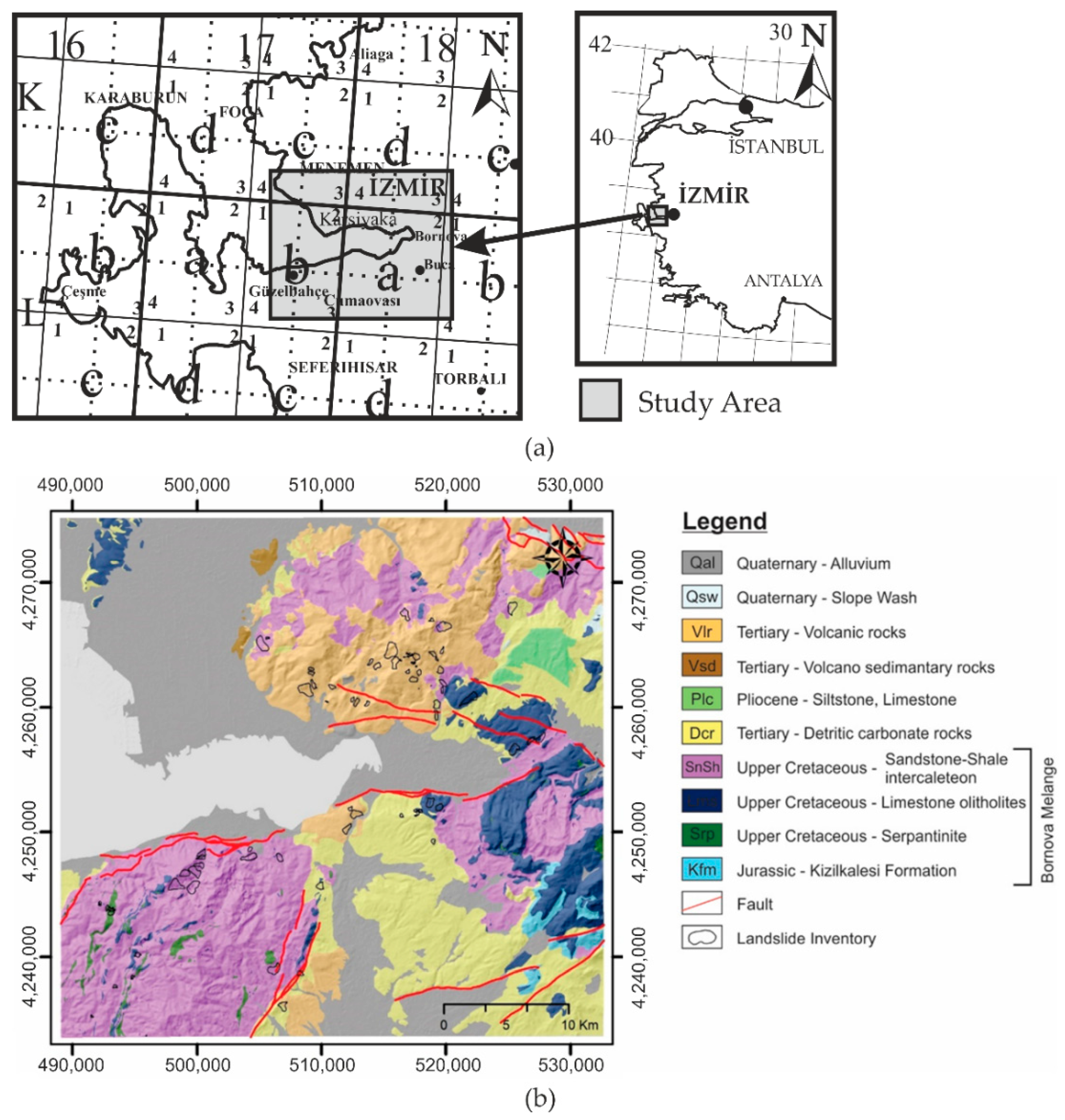
2. Study Area
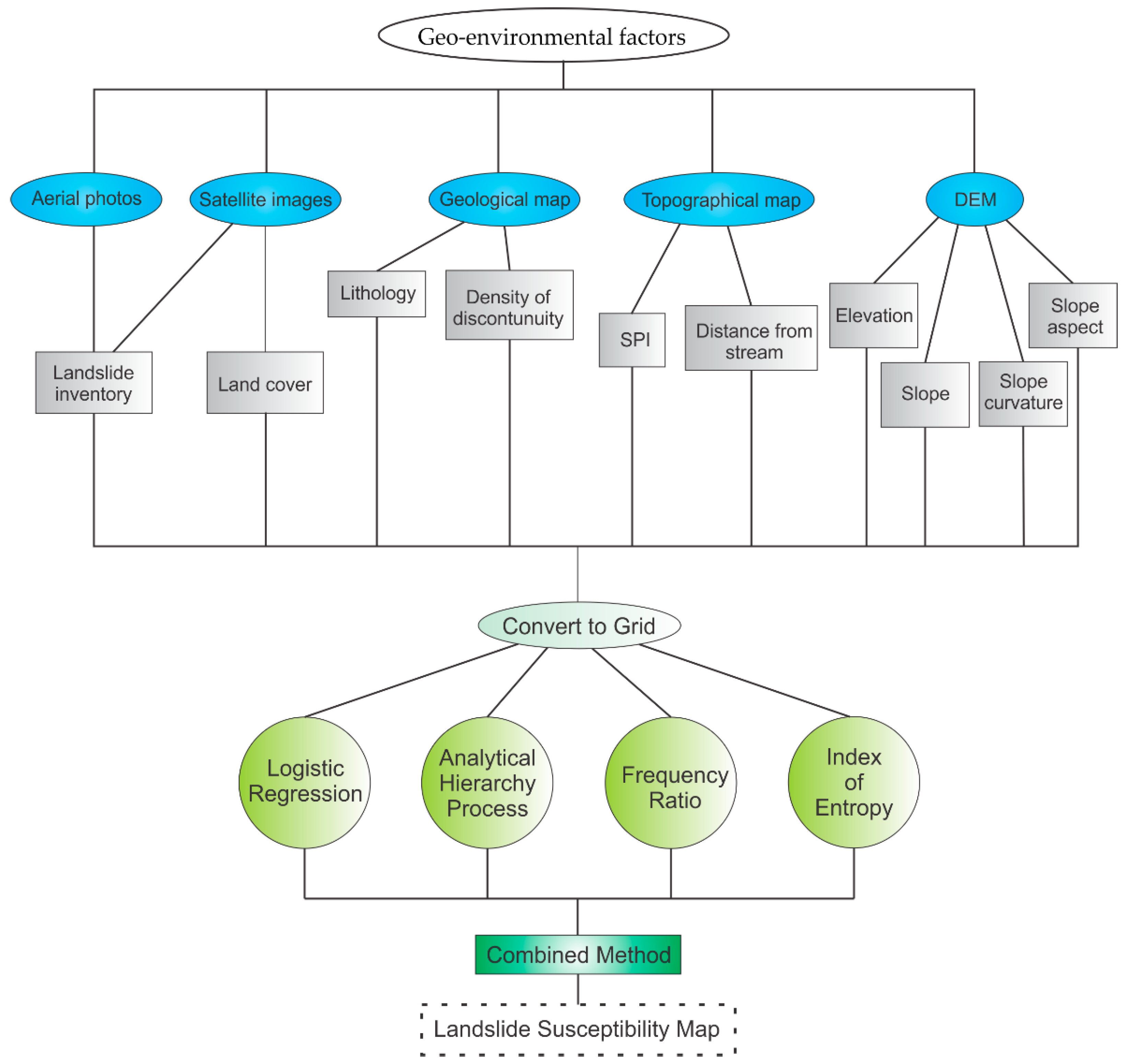
3. Materials and Methods
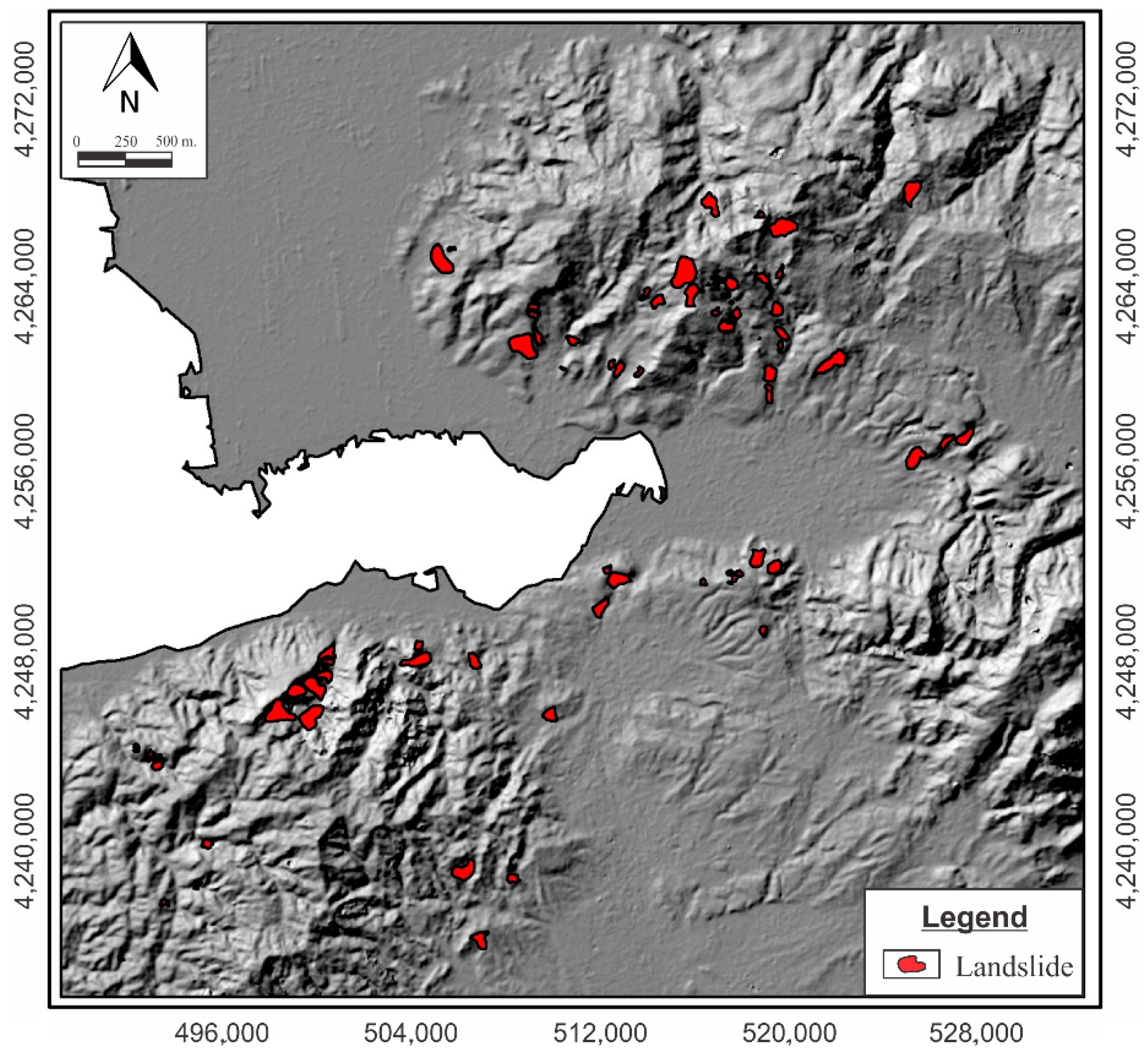
3.1. Landslide Inventory
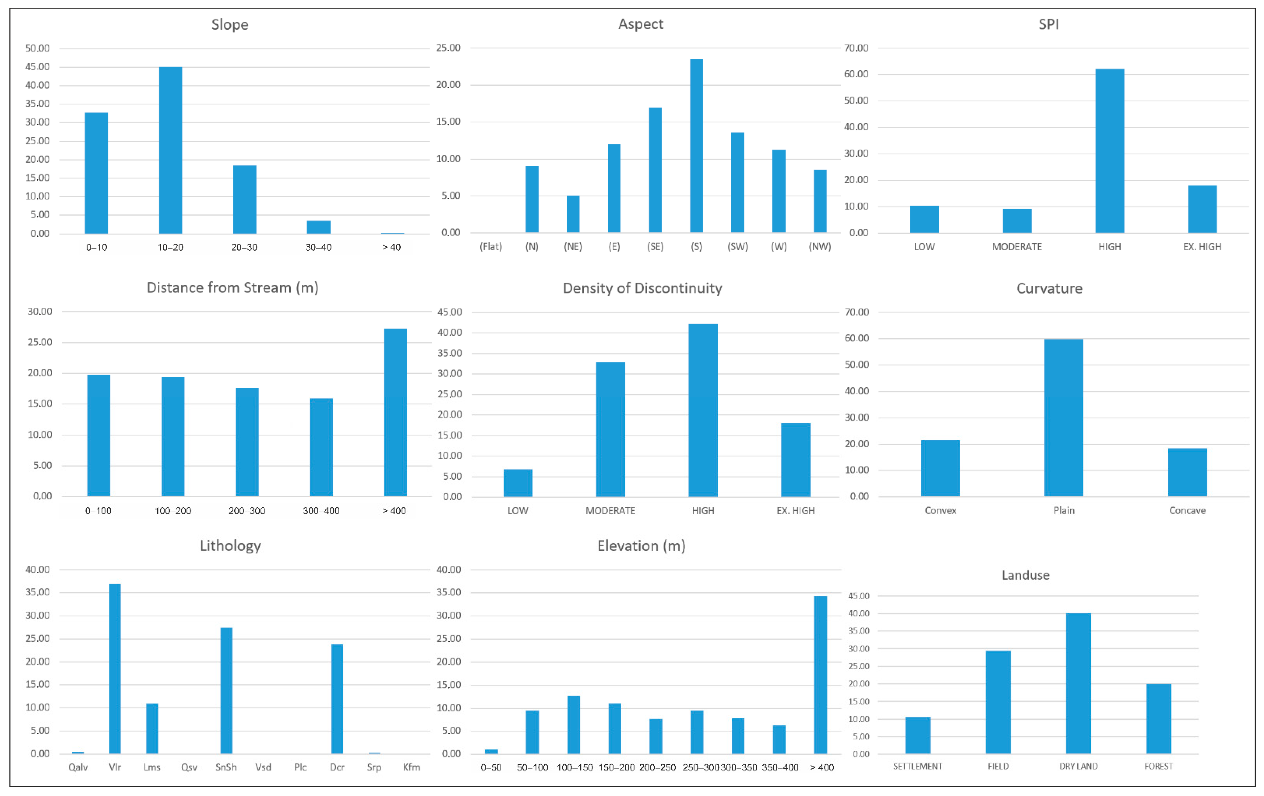
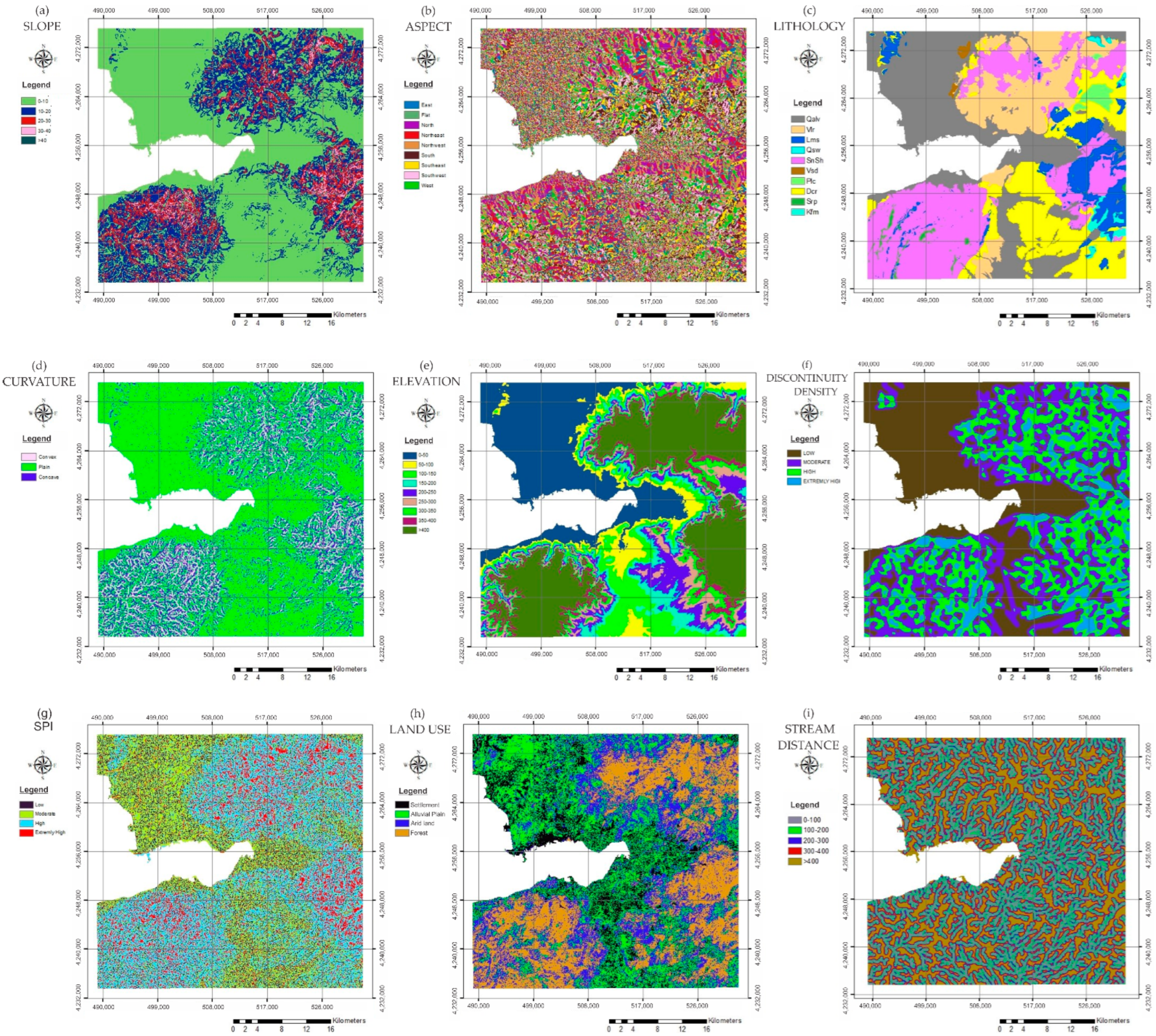
3.2. Geo-Environmental Factors: Definition and Statistical Analysis
3.3. Statistical Analysis
3.3.1. Logistic Regression (LR)
3.3.2. Analytical Hierarchy Process (AHP)
3.3.3. Frequency Ratio (FR)
3.3.4. Index of Entropy (IOE)
3.3.5. Combined Method (CM)
4. Results and Discussion
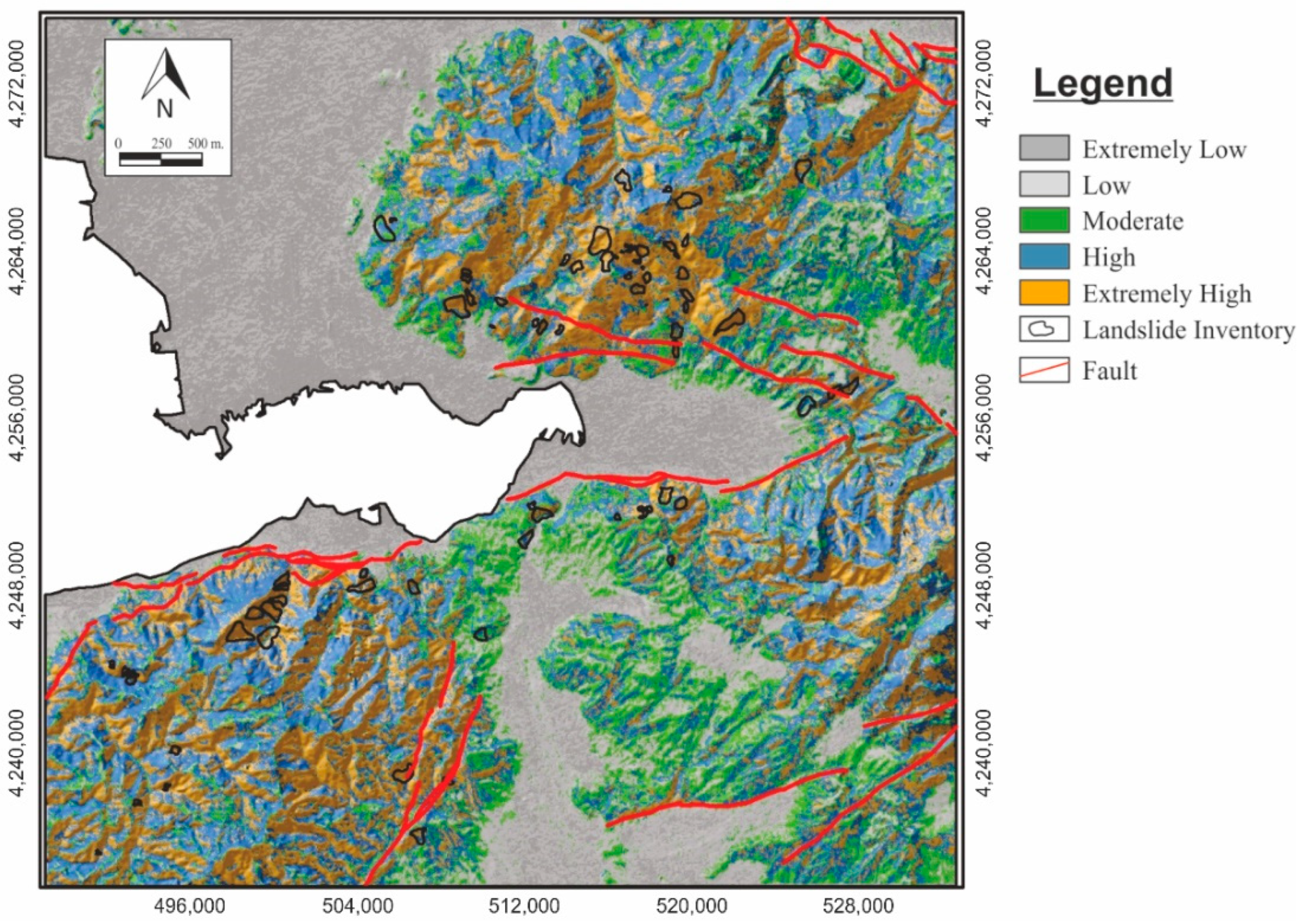
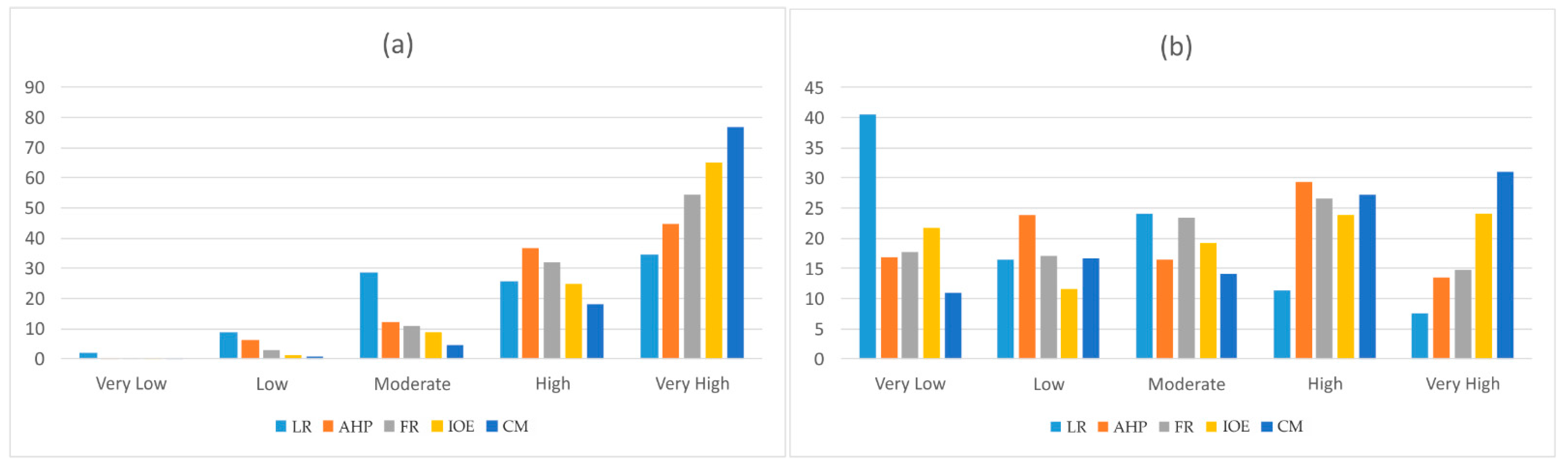
4.1. Comparison of LSM Results
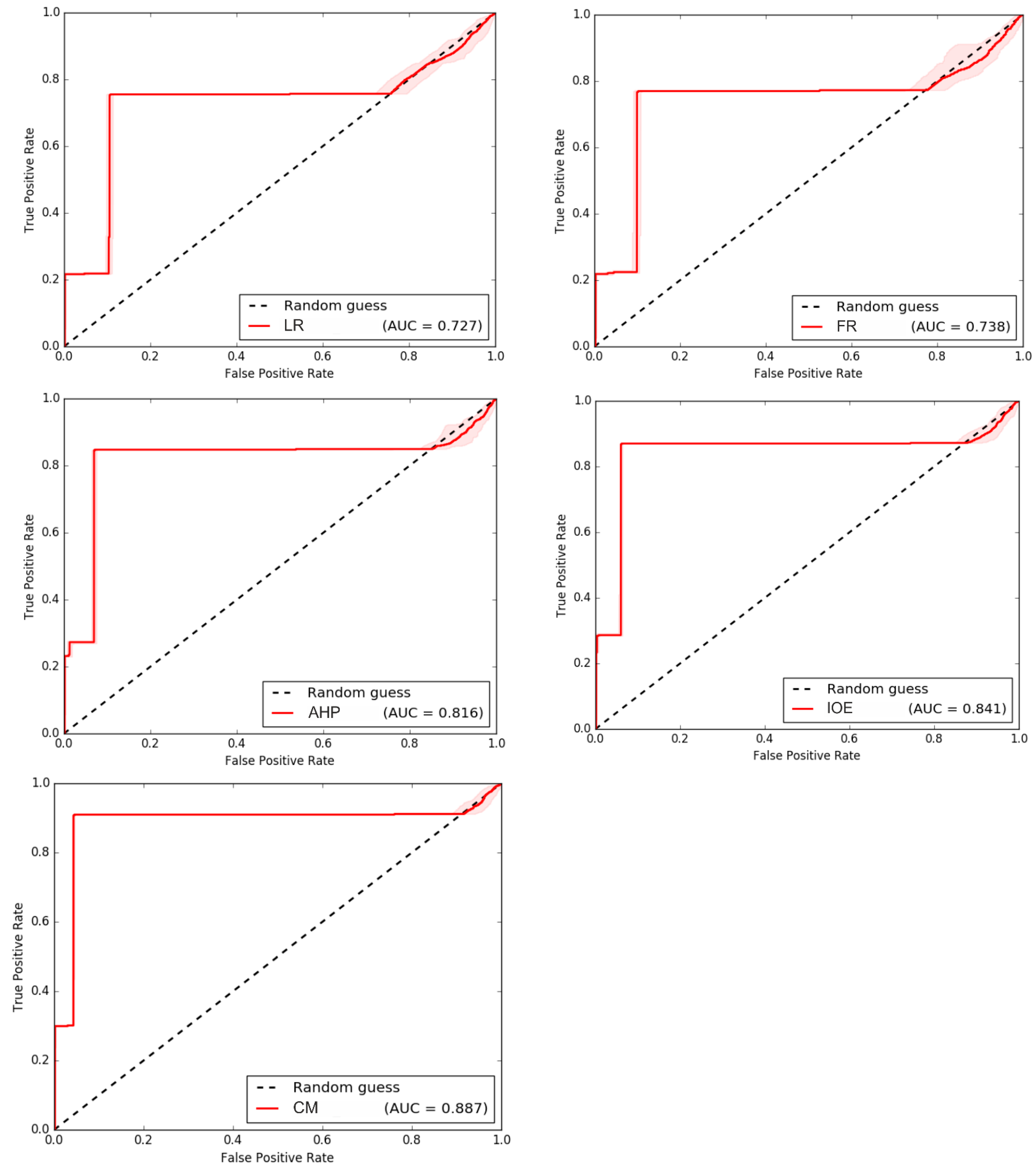
4.2. Evaluation of Model Performance
5. Conclusions
Author Contributions
Funding
Institutional Review Board Statement
Informed Consent Statement
Data Availability Statement
Acknowledgments
Conflicts of Interest
References
- USGS. 2021. Available online: https://www.usgs.gov/faqs/what-landslide-and-what-causes-one (accessed on 3 May 2021).
- Raghuvanshi, T.K. Plane failure in rock slopes—A review on stability analysis techniques. J. King Saud Univ.–Sci. 2019, 31, 101–109. [Google Scholar] [CrossRef]
- Samanta, S.K.; Majumdar, R.K.; Chowdhury, S. Modes of slope failure in layered rocks of landslide zones: Insight from finite element modelling. Indian J. Geosci. 2015, 69, 117–130. [Google Scholar]
- Hack, R.; Alkema, D.; Kruse, G.A.M.; Leenders, N.; Luzi, L. Influence of earthquakes on the stability of slopes. Eng. Geol. 2007, 91, 4–15. [Google Scholar] [CrossRef]
- Park, S.; Kim, W.; Lee, J.; Baek, Y. Case Study on Slope Stability Changes Caused by Earthquakes—Focusing on Gyeongju 5.8 ML EQ. Sustainability 2018, 10, 3441. [Google Scholar] [CrossRef]
- Rupke, J.M.; Huisman, M.; Kruse, H.M.G. Stability of man-made slopes. Eng. Geol. 2007, 91, 16–24. [Google Scholar] [CrossRef]
- Kolapo, P.; Oniyide, G.O.; Said, K.O.; Lawal, A.I.; Onifade, M.; Munemo, P. An Overview of Slope Failure in Mining Operations. Mining 2022, 2, 350–384. [Google Scholar] [CrossRef]
- Çevik, E.; Topal, T. GIS-based landslide susceptibility mapping for a problematic segment of the natural gas pipeline, Hendek (Turkey). Environ. Geol. 2003, 44, 949–962. [Google Scholar] [CrossRef]
- Lee, S. Application of logistic regression model and its validation for landslide susceptibility mapping using GIS and remote sensing data. Int. J. Remote Sens. 2005, 26, 1477–1491. [Google Scholar] [CrossRef]
- Yalcin, A.; Reis, S.; Aydinoglu, A.C.; Yomralioglu, T. A GIS-based comparative study of frequency ratio, analytical hierarchy process, bivariate statistics and logistics regression methods for landslide susceptibility mapping in Trabzon, NE Turkey. CATENA 2011, 85, 274–287. [Google Scholar] [CrossRef]
- Pourghasemi, H.R.; Pradhan, B.; Gokceoglu, C. Application of fuzzy logic and analytical hierarchy process (AHP) to landslide susceptibility mapping at Haraz watershed, Iran. Nat. Hazards 2012, 63, 965–996. [Google Scholar] [CrossRef]
- Shahabi, H.; Khezri, S.; Bin Ahmad, B.; Hashim, M. Landslide susceptibility mapping at central Zab basin, Iran: A comparison between analytical hierarchy process, frequency ratio and logistic regression models. CATENA 2014, 115, 55–70. [Google Scholar] [CrossRef]
- Pham, B.T.; Bui, D.T.; Pourghasemi, H.R.; Indra, P.; Dholakia, M.B. Landslide susceptibility assesssment in the Uttarakhand area (India) using GIS: A comparison study of prediction capability of naïve bayes, multilayer perceptron neural networks, and functional trees methods. Theor. Appl. Climatol. 2017, 128, 255–273. [Google Scholar] [CrossRef]
- Abedini, N.; Tulabi, S. Assessing LNRF, FR, and AHP models in landslide susceptibility mapping index: A comparative study of Nojian watershed in Lorestan province, Iran. Enviromental Earth Sci. 2018, 77, 405. [Google Scholar] [CrossRef]
- Du, G.; Zhang, Y.; Yang, Z.; Guo, C.; Yao, X.; Sun, D. Landslide susceptibility mapping in the region of eastern Himalayan syntaxis, Tibetan Plateau, China: A comparison between analytical hierarchy process information value and logistic regression-information value methods. Bull. Eng. Geol. Environ. 2018, 78, 4201–4215. [Google Scholar] [CrossRef]
- Reichenbach, P.; Rossi, M.; Malamud, B.D.; Mihir, M.; Guzzetti, F. A review of statistically-based landslide susceptibility models. Earth-Sci. Rev. 2018, 180, 60–91. [Google Scholar] [CrossRef]
- Talaei, R.A. Combined Model for Landslide Susceptibility, Hazard and Risk Assessment. AUT J. Civ. Eng. 2018, 2, 11–28. [Google Scholar]
- Carabella, C.; Miccadei, E.; Paglia, G.; Sciarra, N. Post-Wildfire Landslide Hazard Assessment: The Case of the 2017 Montagna Del Morrone Fire (Central Apennines, Italy). Geosciences 2019, 9, 175. [Google Scholar] [CrossRef]
- Demir, G. GIS-based landslide susceptibility mapping for a part of the North Anatolian Fault Zone between Resadiye and Koyulhisar (Turkey). CATENA 2019, 183, 104211. [Google Scholar] [CrossRef]
- Konovalov, A.; Gensiorovskiy, Y.; Lobkina, V.; Muzychenko, A.; Stepnova, Y.; Muzychenko, L.; Stepnov, A.; Mikhalyov, M. Earthquake-Induced Landslide Risk Assessment: An Example from Sakhalin Island, Russia. Geosciences 2019, 9, 305. [Google Scholar] [CrossRef]
- Saha, A.; Mandal, S.; Saha, S. Geo-spatial approach-based landslide susceptibility mapping using analytical hierarchical process, frequency ratio, logistic regression and their ensemble methods. SN Appl. Sci. 2020, 2, 1647. [Google Scholar] [CrossRef]
- Sun, D.; Xu, J.; Wen, H.; Wang, D. Assessment of landslide susceptibility mapping based on Bayesian hyperparameter optimization: A comparison between logistic regression and random forest. Eng. Geol. 2021, 281, 105972. [Google Scholar] [CrossRef]
- Wang, Y.; Frang, Z.; Hong, H.; Costache, R.; Tang, X. Flood susceptibility mapping by integrating frequency ratio and index of entropy with multilayer perceptron and classification and regression tree. J. Environ. Manag. 2021, 289, 112449. [Google Scholar] [CrossRef] [PubMed]
- Carabella, C.; Cinosi, J.; Piattelli, V.; Burrato, P.; Miccadei, E. Earthquake-induced landslides susceptibility evaluation: A case study from the Abruzzo region (Central Italy). CATENA 2022, 208, 105729. [Google Scholar] [CrossRef]
- Melese, T.; Belay, T.; Andemo, A. Application of analytical hierarchal process, frequency ratio, and Shannon entropy approaches for landslide susceptibility mapping using geospatial technology: The case of Dejen district, Ethiopia. Arab. J. Geosci. 2022, 15, 424. [Google Scholar] [CrossRef]
- Chen, W.; Chai, H.; Sun, X.; Wang, Q.; Ding, X.; Hong, H. A GIS-based comparative study of frequency ratio, statistical index and weights-of-evidence models in landslide susceptibility mapping. Arab. J. Geosci. 2016, 9, 204. [Google Scholar] [CrossRef]
- Lee, S.; Min, K. Statistical analysis of landslide susceptibility at Yongin, Korea. Environ. Geol. 2001, 40, 1095–1113. [Google Scholar] [CrossRef]
- Suzen, M.L.; Doyuran, V. A comparison of the GIS based landslide susceptibility assessment methods: Multivariate versus bivariate. Environ. Geol. 2004, 45, 665–679. [Google Scholar] [CrossRef]
- Lee, S.; Ryu, J.H.; Won, J.S.; Park, H.J. Determination and application of the weights for landslide susceptibility mapping using an artificial neural network. Eng. Geol. 2004, 71, 289–302. [Google Scholar] [CrossRef]
- Yılmaz, I. Landslide susceptibility mapping using frequency ratio, logistic regression, artificial neural network sand their comparison: A case study from Kat landslides (Tokat -Turkey). Comput. Geosci. 2009, 7, 1125–1138. [Google Scholar] [CrossRef]
- Suzen, M.L. Data Driven Landslide Hazard Assessment Using Geographical Information System and Remote Sensing. Ph.D. Thesis, Middle East Technical University, Ankara, Turkey, 2002. [Google Scholar]
- Hong, H.; Pourghasemi, H.R.; Pourtaghi, Z.S. Landslide susceptibility assessment in Lianhua County (China): A comparison between a random forest data mining technique and bivariate and multivariate statistical models. Geomorphology 2016, 259, 105–118. [Google Scholar] [CrossRef]
- Degirmenci, I. Entropy Measurement and Maximum Entropy Principle. Master’s Thesis, Hacettepe University, Ankara, Turkey, 2011. [Google Scholar]
- Zadeh, L.A. Shadows of fuzzy sets. Probl. Peredachi Inf. 1965, 2, 37–44. [Google Scholar]
- Bathrellos, G.D.; Skilodimou, H.D.; Chousianitis, K.; Youssef, A.M.; Pradhan, B. Suitability estimation for urban development using multi-hazard assessment map. Sci Total Environ. 2017, 575, 119–134. [Google Scholar] [CrossRef] [PubMed]
- Rahman, M.S.; Ahmed, B.; Di, L. Landslide initiation and runout susceptibility modeling in the context of hill cutting and rapid urbanization: A combined approach of weights of evidence and spatial multi-criteria. J. Mt. Sci. 2017, 14, 1919–1937. [Google Scholar] [CrossRef]
- Achour, Y.; Boumezbeur, A.; Hadji, R.; Chouabbi, A.; Cavaleiro, V.; Bendaoud, E.A. Landslide susceptibility mapping using analytic hierarchy process and information value methods along a highway road section in Constantine, Algeria. Arab. J. Geosci. 2017, 10, 194. [Google Scholar] [CrossRef]
- Sharma, S.; Kumar Mahajan, A. Comparative evaluation of GIS-based landslide susceptibility mapping using statistical and heuristic approach for Dharamshala region of Kangra Valley, India. Geoenviron. Disasters 2018, 5, 4. [Google Scholar] [CrossRef]
- Ali, S.; Biermanns, P.; Haider, R.; Reicherter, K. Landslide susceptibility mapping by using GIS along the China–Pakistan economic corridor (Karakoram Highway), Pakistan. Nat. Hazards Earth Syst. Sci. Discuss. 2018, 19, 999–1022. [Google Scholar] [CrossRef]
- Akgun, A.; Turk, N. Landslide susceptibility mapping for Ayvalik (Western Turkey) and its vicinity by multicriteria decision analysis. Environ. Earth Sci. 2010, 61, 595–611. [Google Scholar] [CrossRef]
- Saaty, T.L.; Vargas, L. The Analytic Network Process. In Decision Making with the Analytic Network Process; Springer: Boston, MA, USA, 2006; pp. 1–26. [Google Scholar] [CrossRef]
- Pradhan, B. A comparative study on the predictive ability of the decision tree, support vector machine and neuro-fuzzy models in landslide susceptibility mapping using GIS. Comput Geosci. 2013, 51, 350–365. [Google Scholar] [CrossRef]
- Shirzadi, A.; Bui, D.T.; Pham, B.T.; Solaimani, K. Shallow landslide susceptibility assessment using a novel hybrid intelligence approach. Environ. Earth Sci. 2017, 76, 60. [Google Scholar] [CrossRef]
- Chen, W.; Li, X.; Wang, Y.; Chen, G.; Liu, S. Forested landslide detection using LiDAR data and the random forest algorithm: A case study of the Three Gorges, China. Remote Sens. Environ. 2014, 152, 291–301. [Google Scholar] [CrossRef]
- Paudel, U.; Oguchi, T.; Hayakawa, Y. Multi-resolution landslide susceptibility analysis using a DEM and random forest. Int. J. Geosci. 2016, 07, 726–743. [Google Scholar] [CrossRef]
- Zhang, K.; Wu, X.; Niu, R.; Yang, K.; Zhao, L. The assessment of landslide susceptibility mapping using random forest and decision tree methods in the three Gorges reservoir area, China. Environ. Earth Sci. 2017, 76, 405. [Google Scholar] [CrossRef]
- Kim, J.; Lee, S.; Jung, H.; Lee, S. Landslide susceptibility mapping using random forest and boosted tree models in Pyeong-Chang, Korea. J. Geocarto Int. 2018, 33, 1000–1015. [Google Scholar] [CrossRef]
- Taalab, K.; Cheng, T.; Zhang, Y. Mapping landslide susceptibility and types using Random Forest. Big Earth Data 2018, 2, 159–178. [Google Scholar] [CrossRef]
- Iovine, G.; Greco, R.; Gariano, S.L.; Pellegrino, A.D.; Terranova, O.G. Shallow-landslide susceptibility in the Costa Viola mountain ridge (Southern Calabria, Italy) with considerations on the role of causal factors. Nat. Hazards 2014, 73, 111–136. [Google Scholar] [CrossRef]
- Karimi Sangchini, E.K.; Emami, S.N.; Tahmasebipour, N.; Pourghasemi, H.R.; Naghibi, S.A.; Wu, Z.; Wu, Y.; Yang, Y.; Chen, F.; Zhang, N.; et al. A comparative study on the landslide susceptibility mapping using logistic regression and statistical index models. Arab. J. Geosci. 2017, 10, 187. [Google Scholar]
- Polykretis, C.; Faka, A.; Chalkias, C. Exploring the Impact of Analysis Scale on Landslide Susceptibility Modeling: Empirical Assessment in Northern Peloponnese, Greece. Geosciences 2018, 8, 261. [Google Scholar] [CrossRef]
- Atkinson, P.M.; Massari, R. Generalized linear modelling of landslide susceptibility in the Central Apennines, Italy. Comput. Geosci. 1998, 24, 373–385. [Google Scholar] [CrossRef]
- Dai, F.C.; Lee, C.F. Landslide characteristics and slope instability modeling using GIS, Lantau Island, Hong Kong. Geomorphology 2002, 42, 213–228. [Google Scholar] [CrossRef]
- Akgun, A.; Bulut, F. GIS-based landslide susceptibility for Arsin-Yomra (Trabzon, North Turkey) region. Environ. Geol. 2007, 51, 1377–1387. [Google Scholar] [CrossRef]
- Akgun, A. A comparison of landslide susceptibility maps produced by logistic regression, multi-criteria decision, and likelihood ratio methods: A case study at İzmir, Turkey. Landslides 2012, 9, 93–106. [Google Scholar] [CrossRef]
- Akgun, A.; Kıncal, C.; Pradhan, B. Application of remote sensing data and GIS for landslide risk assessment as an environmental threat to Izmir city (west Turkey). Environ. Monit. Assess. 2012, 184, 5453–5470. [Google Scholar] [CrossRef] [PubMed]
- Kıncal, C.; Akgun, A.; Koca, M.Y. Landslide susceptibility assessment in the Izmir (West Anatolia, Turkey) city center and its near vicinity by the logistic regression method. Environ. Earth Sci. 2009, 59, 745–756. [Google Scholar] [CrossRef]
- Pradhan, B.; Lee, S.; Buchroithner, M.F. Use of geospatial data for the development of fuzzy algebraic operators to landslide hazard mapping: A case study in Malaysia. Appl. Geomat. 2009, 1, 3–15. [Google Scholar] [CrossRef]
- Gorsevski, P.V.; Brown, M.K.; Panter, K.; Onasch, C.M. Landslide detection and susceptibility mapping using LiDAR and an artificial neural network approach: A case study in the Cuyahoga Valley National Park, Ohio. Landslides 2016, 13, 467–484. [Google Scholar] [CrossRef]
- Crozier, M.J.; Glade, T. Landslide Hazard and Risk: Issues, Concepts and Approach; Glade, T., Anderson, M.G., Crozier, M.J., Eds.; Landslide Risk Assessment; John Wiley: New York, NY, USA, 2005; pp. 1–40. [Google Scholar] [CrossRef]
- Yüksel, N. Usage of Statistical Methods and Artificial Neural Networks in Geographical Information Systems Based Landslide Susceptibility Mapping: Kumluca-Ulus (Bartın-Türkiye) Region. Ph.D. Thesis, Hacettepe University, Institute of Natural and Applied Sciences, Ankara, Turkey, 2007. (In Turkish). [Google Scholar]
- Tantuğ, A.C.; ve Türkmenoğlu, C. Türkçe Metinlerde Duygu Analizi. Master’s Thesis, İstanbul Teknik Üniversitesi, İstanbul, Turkey, 2015. [Google Scholar]
- Çelik, O. A Research on Machine Learning Methods and Its Applications. J. Educ. Technol. Online Learn. 2018, 1, 25–40. [Google Scholar] [CrossRef]
- Do, H.M.; Kun, L.Y.; Zi, Z.G. A comparative study on the integrative ability of the analytical hierarchy process, weights of evidence and logistic regression methods with the Flow-R model for landslide susceptibility assessment. Geomat. Nat. Hazards Risk 2020, 11, 2449–2485. [Google Scholar] [CrossRef]
- Fang, Z.; Wang, Y.; Peng, L.; Hong, H. A comparative study of heterogeneous ensemble-learning techniques for landslide susceptibility mapping. Int. J. Geogr. Inf. Sci. 2020, 35, 321–347. [Google Scholar] [CrossRef]
- Arabameri, A.; Pradhan, B.; Rezaei, K.; Lee, S.; Sohrabi, M. An ensemble model for landslide susceptibility mapping in a forested area. Geocarto Int. 2020, 35, 1680–1705. [Google Scholar] [CrossRef]
- Iban, C.M.; Sekertekin, A. Machine learning based wildfire susceptibility mapping using remotely sensed fire data and GIS: A case study of Adana and Mersin provinces, Turkey. Ecol. Inform. 2022, 69, 101647. [Google Scholar] [CrossRef]
- Saleh, A.; Yuzir, A.; Sabtu, N.; Abujayyab, S.K.M.; Bunmi, M.R.; Pham, Q.B. Flash flood susceptibility mapping in urban area using genetic algorithm and ensemble method. Geocarto Int. 2022, 1–30. [Google Scholar] [CrossRef]
- Arabameri, A.; Pal, S.C.; Costache, R.; Saha, A.; Rezaie, F.; Danesh, A.S.; Pradhan, B.; Lee, S.; Hoang, N.D. Prediction of gully erosion susceptibility mapping using novel ensemble machine learning algorithms. Geomat. Nat. Hazards Risk 2021, 1, 469–498. [Google Scholar] [CrossRef]
- Izmir Governorship. Available online: http://www.izmir.gov.tr/istatistiklerle-izmir (accessed on 8 September 2020).
- MGM, Turkish State Meteorological Service. Available online: https://www.mgm.gov.tr/veridegerlendirme/il-ve-ilceler-istatistik.aspx?k=A&m=IZMIR (accessed on 8 September 2020).
- Kıncal, C. Engineering Geological Evaluation of Geological Units Outcrop in and around the Izmir City Centre with the Help of Geographical Information Systems and Remote Sensing Techniques. Ph.D. Thesis, The Graduate School of Natural and Applied Sciences, Dokuz Eylul University, Izmir, Turkey, 2005; p. 342. (In Turkish). [Google Scholar]
- Erdogan, B. Tectonic Relations between İzmir-Ankara Zone and Karaburun Belt. Bull. Turk. Assoc. Pet. Geol. 1990, 2, 20. [Google Scholar]
- Ersoy, E.Y.; Dindi, F.; Karaoğlu, Ö.; Helvacı, C. Geochemical and petrographic features of the Miocene volcanism around Soma basin, western Anatolia, Turkey. Earth Sci. 2012, 33, 59–80. [Google Scholar]
- GDMRE. Geological Map of Turkey 2000. 1.25000-Scaled Izmir Sheet; General Directorate of Mineral Research and Exploration of Turkey: Ankara, Turkey, 2000.
- Genc, S.C.; Altunkaynak, S.; Karacik, Z.; Yazman, M.; Yılmaz, Y. The Çubukludağ graben, South of Izmir: Tectonic significance in the Neogene geological evolution of the Western Anatolia. Geodin. Acta 2001, 14, 1–12. [Google Scholar]
- Akartuna, M. On the geology of Izmir, Torbalı, Seferhisar, Urla districts. MTA Bull. 1962, 59, 1–19. [Google Scholar]
- Chung, C.-J.F.; Fabbri, A.G. Probabilistic Prediction Models for Landslide Hazard Mapping. Photogramm. Eng. Remote Sens. 1999, 65, 1389–1399. [Google Scholar]
- Choi, J.; Oh, H.J.; Lee, H.J.; Lee, C.; Lee, S. Combining landslide susceptibility maps obtained from frequency ratio, logistic regression, and artificial neural network models using aster images and GIS. Eng. Geol. 2011, 124, 12–23. [Google Scholar] [CrossRef]
- Umar, Z.; Pradhan, B.; Ahmad, A.; Jebur, M.N.; Tehrany, M.S. Earthquake induced landslide susceptibility mapping using an integrated ensemble frequency ratio and logistic regression models in West Sumatera Province, Indonesia. CATENA 2014, 118, 124–135. [Google Scholar] [CrossRef]
- Avsar, M. General Assessment of Landslides in Izmir Metropolitan Area. Master’s Thesis, The Graduate School of Natural and Applied Sciences, Dokuz Eylul University, Izmir, Turkey, 1997. [Google Scholar]
- GDMRE. GeoScience Map Viewer and Drawing Editor. General Directorate of Mineral Research and Exploration of Turkey. Available online: http://yerbilimleri.mta.gov.tr/anasayfa.aspx (accessed on 9 March 2020).
- Carrara, A.; Guzzetti, F.; Cardinali, M.; Reichenbach, P. Use of GIS technology in the prediction and monitoring of landslide hazard. Nat. Hazards 1999, 20, 117–135. [Google Scholar] [CrossRef]
- Guzzetti, F.; Carrara, A.; Cardinali, M.; Reichenbach, P. Landslide hazard evaluation: A review of current techniques and their application in a multi-scale study, Central Italy. Geomorphology 1999, 31, 181–216. [Google Scholar] [CrossRef]
- Soeters, R.; Van Westen, C.J. Slope instability recognition, analysis and zonation. Landslides Investig. Mitig. 1996, 247, 129–177. [Google Scholar]
- Djukem, W.D.L.; Braun, A.; Wouatong, A.S.L.; Guedjeo, C.; Dohmen, K.; Wotchoko, P.; Fernandes-Steeger, T.M.; Havenith, H.B. Effect of soil geomechanical properties and geo-environmental factors on landslide predisposition at mount oku, cameroon. Int. J. Environ. Res. Public Health 2020, 17, 6795. [Google Scholar] [CrossRef] [PubMed]
- ASTER GDEM. Available online: http://earthexplorer.usgs.gov (accessed on 10 June 2020).
- Google Earth Satellite Images. Available online: https://earth.google.com/web/ (accessed on 10 May 2021).
- Cellek, S. Effect of the slope angle and its classification on landslides. Himal. Geol. 2022, 43, 85–95. [Google Scholar]
- Galli, M.; Francesca, A.; Cardinali, M.; Guzzetti, F.; Reichenbach, P. Comparing landslide inventory maps. Geomorphology 2008, 94, 268–289. [Google Scholar] [CrossRef]
- Lee, S.; Dan, N.T. Probabilistic landslide susceptibility mapping in the Lai Chau province of Vietnam: Focus on the relationship between tectonic fractures and landslides. Environ. Geol. 2005, 48, 778–787. [Google Scholar] [CrossRef]
- Yalcin, A.; Bulut, F. Landslide susceptibility mapping using GIS and digital photogrammetric techniques: A case study from Ardeşen (NE-Turkey). Nat. Hazards 2007, 41, 201–226. [Google Scholar] [CrossRef]
- Costanzo, D.; Rotigliano, E.; Irigaray, C.; Jiménez-Perálvarez, J.D.; Chacón, J. Factors selection in landslide susceptibility modelling on large scale following the gis matrix method: Application to the river Beiro basin (Spain). Nat. Hazards Earth Syst. Sci. 2012, 12, 327–340. [Google Scholar] [CrossRef]
- Pradhan, B.; Lee, S. Landslide susceptibility assessment and factor effect analysis: Backpropagation artificial neural networks and their comparison with frequency ratio and bivariate logistic regression modelling. Environ. Modeling Softw. 2010, 25, 747–759. [Google Scholar] [CrossRef]
- ArcMap. Software Manual 2020. Available online: https://arcmap.nersc.no/pdfs/User-Manual-ARCMAP-05-2020-English.pdf (accessed on 5 May 2020).
- Ohlmacher, G.C. Plan curvature and landslide probability in regions dominated by earth flows and earth slides. Eng. Geol. 2007, 91, 117–134. [Google Scholar] [CrossRef]
- Catani, F.; Lagomarsino, D.; Segoni, S.; Tofani, V. Landslide susceptibility estimation by random forests technique: Sensitivity and scaling issues. Nat. Hazards Earth Syst. Sci. 2013, 13, 2815–2831. [Google Scholar] [CrossRef]
- Bastug, G. Preperation of Landslide Susceptibilty Map of Adrasan and Olimpos (Antalya) Regions. Master’s Thesis, Hacettepe University, Ankara, Turkey, 2018. [Google Scholar]
- Tetik Bicer, C. A Semi-Quantitative Evaluation of Landslide Risk Mapping. Ph.D. Thesis, Hacettepe University, Ankara, Turkey, 2017. [Google Scholar]
- Zezere, J.L. Landslide susceptibility assessment considering landslide typology. A case study in the area north of Lisbon (Portugal). Nat. Hazards Earth Syst. Sci. 2002, 2, 73–82. [Google Scholar] [CrossRef]
- Ayalew, L.; Yamagishi, H. The application of GIS-based logistic regression for susceptibility mapping in the Kakuda-Yahiko Mountains, Central Japan. Geomorphology 2005, 65, 15–31. [Google Scholar] [CrossRef]
- Bai, S.B.; Wang, J.; Lü, G.N.; Zhou, P.G.; Hou, S.S.; Xu, S.N. GIS-based logistic regression for landslide susceptibility mapping of the Zhongxian segment in the Three Gorges area, China. Geomorphology 2010, 115, 23–31. [Google Scholar] [CrossRef]
- Lee, S.; Pradhan, B. Landslide hazard mapping at Selangor, Malaysia using frequency ratio and logistic regression models. Landslides 2007, 4, 33–41. [Google Scholar] [CrossRef]
- Idrisi. Software Manual 2020. Available online: https://clarklabs.org/wp-content/uploads/2020/05/Terrset-Manual.pdf (accessed on 5 May 2020).
- Clark, W.A.V.; Hosking, P.L. Statistical methods for geographers. Cah. Géographie Québec 1986, 31, 91–92. [Google Scholar]
- Saaty, T.L. The Analytical Hierarchy Processes; McGraw-Hill: New York, NY, USA, 1980. [Google Scholar]
- Ayalew, L.; Hiromitsu, Y.; Norimitsu, U. Landslide susceptibility mapping using GIS-based weighted linear combination, the case in Tsugawa area of Agano River, Niigata Prefecture, Japan. Landslides 2004, 1, 73–81. [Google Scholar] [CrossRef]
- Saaty, T.L.; Vargas, L.G. Prediction, Projectionand Forecasting 2008; Kluwer: New York, NY, USA, 1991. [Google Scholar]
- Saaty, T.L. Ascaling method for priorities in hierarchical structure. J. Math. Psychol. 1977, 15, 34–39. [Google Scholar] [CrossRef]
- Malczewski, J. GIS and Multi-Criteria Decision Analysis; John Wiley: New York, NY, USA, 1999. [Google Scholar]
- Lee, S.; Thalib, J.A. Probabilistic landslide susceptibility and factor effect analysis. Environ. Geol. 2005, 47, 982–990. [Google Scholar] [CrossRef]
- Yufeng, S.; Fengxiang, J. Landslide stability analysis based on generalized information entropy. In Proceedings of the 2009 International Conference on Environmental Science and Information Application Technology, Wuhan, China, 4–5 July 2009; pp. 83–85. [Google Scholar] [CrossRef]
- Shannon, C.E. A Mathematical Theory of Communication. Bull. Syst. Technol. J. 1948, 27, 379–423. [Google Scholar] [CrossRef]
- Li, X.; Wang, K.; Liu, L.; Xin, J. Application of the entropy weight and topsis method in safety evaluation of coal mines. Procedia Eng. 2011, 26, 2085–2091. [Google Scholar] [CrossRef]
- Mon, D.L.; Cheng, C.H.; Lin, J.C. Evaluating weapon system using fuzzy analytic hierarchy process based on entropy weight. Fuzzy Sets Syst. 1994, 62, 127–134. [Google Scholar] [CrossRef]
- Ren, L.C. Disaster entropy: Conception and application. J. Nat. Disasters 2000, 9, 26–31. [Google Scholar]
- Yang, Z.; Qiao, J. Entropy-based hazard degree assessment for typical landslides in the Three Gorges Area in “Landslide Disaster Mitigation in Three Gorges Reservoir, China”. Environ. Sci. Eng. 2009, 519–529. [Google Scholar] [CrossRef]
- Youssef, A.M.; Al-Kathery, M.; Pradhan, B. Landslide susceptibility mapping at Al-Hasher Area, Jizan (Saudi Arabia) using GIS-based frequency ratio and index of entropy models. Geosci. J. 2015, 19, 113–134. [Google Scholar] [CrossRef]
- Yang, Z.; Qiao, J.; Zhang, X. Regional Landslide Zonation based on Entropy Method in Three Gorges Area, China. In Proceedings of the Seventh International Conference on Fuzzy Systems and Knowledge Discovery 2010, FSKD 2010, Yantai, China, 10–12 August 2010; pp. 1336–1339. [Google Scholar]
- Bednarik, M.; Magulová, B.; Matys, M.; Marschalko, M. Landslide susceptibility assessment of the Kralovany–Liptovsky Mikuláš railway case study. Phys. Chem. Earth Part A/B/C 2010, 35, 162–171. [Google Scholar] [CrossRef]
- Devkota, K.C.; Regmi, A.D.; Pourghasemi, H.R.; Yoshida, K.; Pradhan, B.; Ryu, I.C.; Althuwaynee, O.F. Landslide susceptibility mapping using certainty factor, index of entropy and logistic regression models in GIS and their comparison at Mugling- Narayanghat road section in Nepal Himalaya. Nat. Hazards 2013, 65, 135–165. [Google Scholar] [CrossRef]
- Chen, T.; Zhu, L.; Niu, R.; Trinder, J.; Peng, L.; Lei, T. Mapping landslide susceptibility at the Three Gorges Reservoir, China, using gradient boosting decision tree, random forest and information value models. J. Mt. Sci. 2020, 17, 670–685. [Google Scholar] [CrossRef]
- Lv, L.; Chen, T.; Dou, J.; Plaza, A. A hybrid ensemble-based deep-learning framework for landslide susceptibility mapping. Int. J. Appl. Earth Obs. Geoinf. 2022, 108, 102713. [Google Scholar] [CrossRef]


| Group | Data Source | Scale/Resolution | Factor | Data Type | |
|---|---|---|---|---|---|
| Geo-environmental factors | Geomorphological factors | ASTER GDEM [87] | 30*30 m | Slope angle | Numerical |
| Slope aspect | Categorical | ||||
| Elevation | Numerical | ||||
| Slope curvature | Categorical | ||||
| Hydrological factors | Topographical map | 1/25,000/25*25 m | SPI | Categorical | |
| Distance from stream | Numerical | ||||
| Geological factors | Geological map | 1/25,000/25*25 m | Lithology | Categorical | |
| Density of ciscontinuity | Categorical | ||||
| Human factor | Satellite images | 30*30 m | Land use | Categorical |
| Statistics | Value |
|---|---|
| Total number of pixels | 2,908,836 |
| −2logL0 | 27,433.052 |
| −2log(likelihood) | 23,025.032 |
| Pseudo-R2 | 0.1607 |
| Goodness of fit | 207,434.51 |
| Area under the ROC curve | 0.727 |
| Importance | Definition | Explanation |
|---|---|---|
| 1 | Equal importance | Contribution to objective is equal |
| 3 | Moderate importance | Attribute is slightly favored over another |
| 5 | Strong importance | Attribute is strongly favored over another |
| 7 | Very strong importance | Attribute is very strongly favored over another |
| 9 | Extreme importance | Evidence favoring one attribute is of the highest possible order of affirmation |
| 2, 4, 6, 8 | Intermediate values | When compromise is needed |
| Reciprocals | Opposites | Used for inverse comparison |
| Parameter | 1 | 2 | 3 | 4 | 5 | 6 | 7 | 8 | 9 | Weight |
|---|---|---|---|---|---|---|---|---|---|---|
| (1) Slope aspect | 1 | 0.1617 | ||||||||
| (2) Density of discontinuity | 1/2 | 1 | 0.1113 | |||||||
| (3) Lithology | 1 | 2 | 1 | 0.1617 | ||||||
| (4) Slope | 2 | 3 | 2 | 1 | 0.2716 | |||||
| (5) SPI | 1/4 | 1/3 | 1/4 | 1/6 | 1 | 0.0458 | ||||
| (6) Slope curvature | 1/5 | 1/4 | 1/5 | 1/7 | 1/2 | 1 | 0.0307 | |||
| (7) Elevation | 1/6 | 1/5 | 1/6 | 1/8 | 1/3 | 1/2 | 1 | 0.0221 | ||
| (8) Land use | 1 | 1 | 1 | 1/2 | 4 | 5 | 6 | 1 | 0.1495 | |
| (9) Distance from stream | 1/4 | 1/3 | 1/4 | 1/6 | 1 | 2 | 3 | 1/4 | 1 | 0.0458 |
| Consistency ratio: 0.03 |
| Factor | Class | No. of Pixels in Domain | Percentage of Domain | No. of Landslide | Percentageof Landslide | FR | Normalized Frequency Ratio |
|---|---|---|---|---|---|---|---|
| Slope (Deg) | 0–10 | 1,527,794 | 60.43 | 14,109 | 32.72 | 0.54 | 0.31 |
| 10–20 | 678,851 | 26.85 | 19,454 | 45.12 | 1.68 | 0.95 | |
| 20–30 | 266,839 | 10.55 | 7966 | 18.47 | 1.75 | 0.99 | |
| 30–40 | 49,548 | 1.96 | 1491 | 3.46 | 1.76 | 1.00 | |
| >40 | 5163 | 0.20 | 100 | 0.23 | 1.14 | 0.65 | |
| Aspect | Flat | 29,326 | 1.16 | 0 | 0.00 | 0.00 | 0.00 |
| N | 312,627 | 12.37 | 3910 | 9.07 | 0.73 | 0.42 | |
| NE | 259,456 | 10.26 | 2174 | 5.04 | 0.49 | 0.28 | |
| E | 247,899 | 9.81 | 5175 | 12.00 | 1.22 | 0.70 | |
| SE | 299,619 | 11.85 | 7315 | 16.96 | 1.43 | 0.82 | |
| S | 338,804 | 13.40 | 10,140 | 23.52 | 1.75 | 1.00 | |
| SW | 330,225 | 13.06 | 5856 | 13.58 | 1.04 | 0.59 | |
| W | 343,688 | 13.59 | 4858 | 11.27 | 0.83 | 0.47 | |
| NW | 366,551 | 14.50 | 3692 | 8.56 | 0.59 | 0.34 | |
| SPI | Low | 434,163 | 17.17 | 4457 | 10.34 | 0.60 | 0.37 |
| Moderate | 667,197 | 26.39 | 3997 | 9.27 | 0.35 | 0.21 | |
| High | 1,145,730 | 45.32 | 26,856 | 62.28 | 1.37 | 0.84 | |
| Ex. high | 281,105 | 11.12 | 7810 | 18.11 | 1.63 | 1.00 | |
| Distance from stream (m) | 0–100 | 628,808 | 24.87 | 8536 | 19.80 | 0.80 | 0.62 |
| 100–200 | 536,113 | 21.21 | 8353 | 19.37 | 0.91 | 0.70 | |
| 200–300 | 450,044 | 17.80 | 7591 | 17.60 | 0.99 | 0.77 | |
| 300–400 | 377,276 | 14.92 | 6863 | 15.92 | 1.07 | 0.83 | |
| >400 | 535,954 | 21.20 | 11,777 | 27.31 | 1.29 | 1.00 | |
| Density of discontinuity | Low | 803,727 | 31.79 | 2925 | 6.78 | 0.21 | 0.11 |
| Moderate | 766,508 | 30.32 | 14,,173 | 32.87 | 1.08 | 0.56 | |
| High | 720,240 | 28.49 | 18236 | 42.29 | 1.48 | 0.77 | |
| Ex. high | 237,720 | 9.40 | 7786 | 18.06 | 1.92 | 1.00 | |
| Curvature | Convex | 367,398 | 14.53 | 9300 | 21.57 | 1.48 | 1.00 |
| Plain | 1,773,818 | 70.16 | 25,822 | 59.88 | 0.85 | 0.57 | |
| Concave | 386,979 | 15.31 | 7998 | 18.55 | 1.21 | 0.82 | |
| Lithology | Qalv | 750,212 | 29.71 | 213 | 0.49 | 0.02 | 0.00 |
| Vlr | 362,782 | 14.37 | 15,952 | 36.99 | 2.57 | 1.00 | |
| Lms | 201,654 | 7.99 | 4715 | 10.93 | 1.37 | 0.53 | |
| Qsv | 7848 | 0.31 | 0 | 0.00 | 0.00 | 0.00 | |
| SnSh | 688,762 | 27.28 | 11,822 | 27.42 | 1.00 | 0.39 | |
| Vsd | 9260 | 0.37 | 0 | 0.00 | 0.00 | 0.00 | |
| Plc | 30,337 | 1.20 | 0 | 0.00 | 0.00 | 0.00 | |
| Dcr | 429,522 | 17.01 | 10,267 | 23.81 | 1.40 | 0.55 | |
| Srp | 21,359 | 0.85 | 120 | 0.28 | 0.33 | 0.13 | |
| Kfm | 22,983 | 0.91 | 0 | 0.00 | 0.00 | 0.00 | |
| Elevation (m) | 0–50 | 607,148 | 24.02 | 458 | 1.06 | 0.04 | 0.03 |
| 50–100 | 161,965 | 6.41 | 4105 | 9.52 | 1.49 | 0.94 | |
| 100–150 | 219,961 | 8.70 | 5473 | 12.69 | 1.46 | 0.92 | |
| 150–200 | 175,781 | 6.95 | 4764 | 11.05 | 1.59 | 1.00 | |
| 200–250 | 209,613 | 8.29 | 3342 | 7.75 | 0.93 | 0.58 | |
| 250–300 | 170,361 | 6.74 | 4115 | 9.54 | 1.42 | 0.89 | |
| 300–350 | 154,400 | 6.11 | 3352 | 7.77 | 1.27 | 0.80 | |
| 350–400 | 125,978 | 4.98 | 2701 | 6.26 | 1.26 | 0.79 | |
| >400 | 702,988 | 27.81 | 14,810 | 34.35 | 1.24 | 0.78 | |
| Land use | Settlement | 362,269 | 14.33 | 4607 | 10.68 | 0.75 | 0.51 |
| Field | 731,306 | 28.93 | 12,645 | 29.33 | 1.01 | 0.69 | |
| Dry land | 690,159 | 27.30 | 17,266 | 40.04 | 1.47 | 1.00 | |
| Forest | 742,845 | 29.38 | 8602 | 19.95 | 0.68 | 0.46 |
| Factor | Class | No. of Pixels in Domain | Percentage of Domain | No. of Landslide | Percentage of Landslide | Pij | (Pij) | Hj | Hj max | Ij | Wj |
|---|---|---|---|---|---|---|---|---|---|---|---|
| SLOPE (Deg) | 0–10 | 1,527,794 | 60.43 | 14,109 | 32.72 | 0.54 | 0.08 | 2.23 | 2.32 | 0.04 | 0.05 |
| 10–20 | 678,851 | 26.85 | 19,454 | 45.12 | 1.68 | 0.24 | |||||
| 20–30 | 266,839 | 10.55 | 7966 | 18.47 | 1.75 | 0.25 | |||||
| 30–40 | 49,548 | 1.96 | 1491 | 3.46 | 1.76 | 0.26 | |||||
| >40 | 5163 | 0.20 | 100 | 0.23 | 1.14 | 0.17 | |||||
| Aspect | Flat | 29,326 | 1.16 | 0 | 0.00 | 0.00 | 0.00 | 2.87 | 3.17 | 0.09 | 0.09 |
| N | 312,627 | 12.37 | 3910 | 9.07 | 0.73 | 0.09 | |||||
| NE | 259,456 | 10.26 | 2174 | 5.04 | 0.49 | 0.06 | |||||
| E | 247,899 | 9.81 | 5175 | 12.00 | 1.22 | 0.15 | |||||
| SE | 299,619 | 11.85 | 7315 | 16.96 | 1.43 | 0.18 | |||||
| S | 338,804 | 13.40 | 10,140 | 23.52 | 1.75 | 0.22 | |||||
| SW | 330,225 | 13.06 | 5856 | 13.58 | 1.04 | 0.13 | |||||
| W | 343,688 | 13.59 | 4858 | 11.27 | 0.83 | 0.10 | |||||
| NW | 366,551 | 14.50 | 3692 | 8.56 | 0.59 | 0.07 | |||||
| SPI | Low | 434,163 | 17.17 | 4457 | 10.34 | 0.60 | 0.15 | 1.78 | 2.00 | 0.11 | 0.11 |
| Moderate | 667,197 | 26.39 | 3997 | 9.27 | 0.35 | 0.09 | |||||
| High | 1,145,730 | 45.32 | 26,856 | 62.28 | 1.37 | 0.35 | |||||
| Ex. high | 281,105 | 11.12 | 7810 | 18.11 | 1.63 | 0.41 | |||||
| Distance from stream (m) | 0–100 | 628,808 | 24.87 | 8536 | 19.80 | 0.80 | 0.16 | 2.31 | 2.32 | 0.00 | 0.00 |
| 100–200 | 536,113 | 21.21 | 8353 | 19.37 | 0.91 | 0.18 | |||||
| 200–300 | 450,044 | 17.80 | 7591 | 17.60 | 0.99 | 0.20 | |||||
| 300–400 | 377,276 | 14.92 | 6863 | 15.92 | 1.07 | 0.21 | |||||
| >400 | 535,954 | 21.20 | 11,777 | 27.31 | 1.29 | 0.26 | |||||
| Density of discontinuity | Low | 803,727 | 31.79 | 2925 | 6.78 | 0.21 | 0.05 | 1.75 | 2.00 | 0.13 | 0.15 |
| Moderate | 766,508 | 30.32 | 14,173 | 32.87 | 1.08 | 0.23 | |||||
| High | 720,240 | 28.49 | 18,236 | 42.29 | 1.48 | 0.32 | |||||
| Ex. high | 237,720 | 9.40 | 7786 | 18.06 | 1.92 | 0.41 | |||||
| Curvature | Convex | 367,398 | 14.53 | 9300 | 21.57 | 1.48 | 0.42 | 1.55 | 1.59 | 0.03 | 0.03 |
| Plain | 1,773,818 | 70.16 | 25,822 | 59.88 | 0.85 | 0.24 | |||||
| Concave | 386,979 | 15.31 | 7998 | 18.55 | 1.21 | 0.34 | |||||
| Lithology | Qalv | 750,212 | 29.71 | 213 | 0.49 | 0.02 | 0.00 | 2.19 | 3.32 | 0.34 | 0.23 |
| Vlr | 362,782 | 14.37 | 15,952 | 36.99 | 2.57 | 0.38 | |||||
| Lms | 201,654 | 7.99 | 4715 | 10.93 | 1.37 | 0.20 | |||||
| Qsv | 7848 | 0.31 | 0 | 0.00 | 0.00 | 0.00 | |||||
| SnSh | 688,762 | 27.28 | 11,822 | 27.42 | 1.00 | 0.15 | |||||
| Vsd | 9260 | 0.37 | 0 | 0.00 | 0.00 | 0.00 | |||||
| Plc | 30,337 | 1.20 | 0 | 0.00 | 0.00 | 0.00 | |||||
| Dcr | 429,522 | 17.01 | 10,267 | 23.81 | 1.40 | 0.21 | |||||
| Srp | 21,359 | 0.85 | 120 | 0.28 | 0.33 | 0.05 | |||||
| Kfm | 22,983 | 0.91 | 0 | 0.00 | 0.00 | 0.00 | |||||
| Elevation (m) | 0–50 | 607,148 | 24.02 | 458 | 1.06 | 0.04 | 0.00 | 3.10 | 3.17 | 0.02 | 0.03 |
| 50–100 | 161,965 | 6.41 | 4105 | 9.52 | 1.49 | 0.14 | |||||
| 100–150 | 219,961 | 8.70 | 5473 | 12.69 | 1.46 | 0.14 | |||||
| 150–200 | 175,781 | 6.95 | 4764 | 11.05 | 1.59 | 0.15 | |||||
| 200–250 | 209,613 | 8.29 | 3342 | 7.75 | 0.93 | 0.09 | |||||
| 250–300 | 170,361 | 6.74 | 4115 | 9.54 | 1.42 | 0.13 | |||||
| 300–350 | 154,400 | 6.11 | 3352 | 7.77 | 1.27 | 0.12 | |||||
| 350–400 | 125,978 | 4.98 | 2701 | 6.26 | 1.26 | 0.12 | |||||
| >400 | 702,988 | 27.81 | 14,810 | 34.35 | 1.24 | 0.12 | |||||
| Land use | Settlement | 362,269 | 14.33 | 4607 | 10.68 | 0.75 | 0.19 | 1.93 | 2.00 | 0.04 | 0.03 |
| Field | 731,306 | 28.93 | 12,645 | 29.33 | 1.01 | 0.26 | |||||
| Dry land | 690,159 | 27.30 | 17,266 | 40.04 | 1.47 | 0.38 | |||||
| Forest | 742,845 | 29.38 | 8602 | 19.95 | 0.68 | 0.17 |
| Extremely Low | Low | Moderate | High | Extremely High | |
|---|---|---|---|---|---|
| LR | 2.07% | 8.84% | 28.82% | 25.57% | 34.7% |
| AHP | 0.19% | 6.27% | 12.01% | 36.7% | 44.84% |
| FR | 0.18% | 2.72% | 10.93% | 31.88% | 54.29% |
| IOE | 0.17% | 1.32% | 8.71% | 24.69% | 65.11% |
| CM | 0% | 0.65% | 4.42% | 18.09% | 76.84% |
| Parameter | 1 | 2 | 3 | 4 | 5 | 6 | 7 | 8 | 9 |
|---|---|---|---|---|---|---|---|---|---|
| (1) Slope aspect | 1 | ||||||||
| (2) Density of discontinuity | −0.16 | 1 | |||||||
| (3) Lithology | −0.40 | 0.65 | 1 | ||||||
| (4) Slope | −0.55 | 0.66 | 0.47 | 1 | |||||
| (5) SPI | 0.46 | 0.59 | −0.03 | −0.03 | 1 | ||||
| (6) Slope curvature | 0.68 | 0.05 | −0.24 | 0.04 | −0.04 | 1 | |||
| (7) Elevation | −0.48 | 0.45 | 0.15 | 0.65 | −0.27 | −0.61 | 1 | ||
| (8) Land use | −0.31 | −0.10 | 0.38 | 0.48 | −0.68 | 0.47 | 0.30 | 1 | |
| (9) Distance from stream | −0.43 | −0.48 | 0.41 | −0.41 | −0.67 | −0.69 | 0.23 | 0.18 | 1 |
| CM | LR | AHP | FR | IOE | |
|---|---|---|---|---|---|
| Mean | 3.2573 | 2.3028 | 3.0243 | 3.0641 | 3.2090 |
| Standard Error | 0.0174 | 0.0164 | 0.0164 | 0.0165 | 0.0182 |
| Median | 4 | 2 | 3 | 3 | 3 |
| Mode | 4 | 1 | 4 | 4 | 5 |
| Standard Deviation | 1.3845 | 1.3037 | 1.3021 | 1.3149 | 1.4452 |
| Sample Variance | 1.9168 | 1.6998 | 1.6956 | 1.7290 | 2.0886 |
| Kurtosis | −1.23344 | −0.864065733 | −1.207652717 | −1.106893346 | −1.25068 |
| Skewness | −0.26904 | 0.559431068 | −0.093076809 | −0.161480185 | −0.28333 |
| Range | 4 | 4 | 4 | 4 | 4 |
| Minimum | 1 | 1 | 1 | 1 | 1 |
| Maximum | 5 | 5 | 5 | 5 | 5 |
| Sum | 20.476 | 14.476 | 19.011 | 19.261 | 20.172 |
| Count | 6286 | 6286 | 6286 | 6286 | 6286 |
Publisher’s Note: MDPI stays neutral with regard to jurisdictional claims in published maps and institutional affiliations. |
© 2022 by the authors. Licensee MDPI, Basel, Switzerland. This article is an open access article distributed under the terms and conditions of the Creative Commons Attribution (CC BY) license (https://creativecommons.org/licenses/by/4.0/).
Share and Cite
KINCAL, C.; KAYHAN, H. A Combined Method for Preparation of Landslide Susceptibility Map in Izmir (Türkiye). Appl. Sci. 2022, 12, 9029. https://doi.org/10.3390/app12189029
KINCAL C, KAYHAN H. A Combined Method for Preparation of Landslide Susceptibility Map in Izmir (Türkiye). Applied Sciences. 2022; 12(18):9029. https://doi.org/10.3390/app12189029
Chicago/Turabian StyleKINCAL, Cem, and Hakan KAYHAN. 2022. "A Combined Method for Preparation of Landslide Susceptibility Map in Izmir (Türkiye)" Applied Sciences 12, no. 18: 9029. https://doi.org/10.3390/app12189029
APA StyleKINCAL, C., & KAYHAN, H. (2022). A Combined Method for Preparation of Landslide Susceptibility Map in Izmir (Türkiye). Applied Sciences, 12(18), 9029. https://doi.org/10.3390/app12189029