Conservation Laws and Travelling Wave Solutions for a Negative-Order KdV-CBS Equation in 3+1 Dimensions

Abstract

In this paper, we study a new negative-order KdV-CBS equation in $(3+1)$ dimensions which is a combination of the Korteweg-de Vries (KdV) equation and Calogero–Bogoyavlenskii–Schiff (CBS) equation. Firstly, we determine the Lie point symmetries of the equation and conservation laws by using the multiplier method. The conservation laws will be used to obtain a triple reduction to a second order ordinary differential equation (ODE), which lead to line travelling waves and soliton solutions. Such solitons are obtained via the modified form of simple equation method and are displayed through three-dimensional plots at specific parameter values to lend physical meaning to nonlinear phenomena. It illustrates that these solutions might be extremely beneficial in understanding physical phenomena in a variety of applied mathematics areas.

1. Introduction

The analysis of higher-dimensional nonlinear systems, particularly integrable systems, has exploded in popularity in recent years. Solitary waves theory finds applications in a wide range of scientific domains, including telecommunications, transport phenomena, ocean waves, quantum mechanics, plasma physics, nonlinear fibre optics, and many more. In latest years, research into generating higher-dimensional integrable equations has gotten greater attention, with various integrable models established in the setting of (2+1) and (3+1)-dimensional equations [1,2]. The domain of integrable equations is crucial to investigate as it clarifies the true nature of nonlinearity in science disciplines and reveals its scientific nature.

A variety of chemical, biological and physical phenomena are modeled via nonlinear partial differential equations (PDEs) which contribute a key role in nonlinear science [3]. It provides an abundance of physical data and a deeper understanding of the problem’s physical characteristics, resulting in additional applications [4,5,6,7]. Many tracks have been established for physical issues in recent years in order to come up with exact solutions for nonlinear PDEs using modern computer technologies. There are a number of effective approaches, for instance, the modified extended tanh-function technique [8], the extended modified auxiliary equation mapping method [9,10], the Riccati–Bernoulli Sub-ODE technique [11], the auxiliary equation technique [12], the $(G^{\prime }/G)$-expansion technique [13], homotopy perturbation technique [14], the unified technique [15], the generalized unified technique [16], modified simple equation technique [17], the extended trial function technique [18], the homogeneous balance technique [19], the extended direct algebraic technique [20], the modified extended direct algebraic technique [21] and the collective variable technique [22].

Among the most powerful strategies for constructing nonlinear PDEs solutions is Lie group transformations theory. The investigation of the invariance property of a particular differential equation under a continuous group of transformations is the core principle behind this theory. The application of Lie symmetry transformation technique to PDEs, results in reductions and invariant solutions. Invariant solutions are frequently employed to investigate analytical features. Conservation laws are well acknowledged to participate actively in the solution of a PDE. Not all PDEs obeying conservation laws have physical interpretations, but they are crucial in investigating the integrability of PDEs.

In a wide range of scientific and technical domains, the classical Lie symmetry theory is frequently used [23,24]. This idea was originally suggested by a mathematician named Sophus Lie in the early nineteenth century [25,26]. It has significantly increased applications in nonlinear PDEs and has proven beneficial in various fields of differential equations [27]. The fundamental purpose underlying Lie group theory is to use the invariance requirement of nonlinear PDEs to achieve the similarity variable and reduction equation, and subsequently to derive similarity and solitary wave solutions [28]. These solutions explain a fundamental and significant physical phenomenon. The Chen–Lee–Liu equation, Sawada–Kotera equation, Boussinesq equation, and many more models have recently been studied using the Lie symmetry technique [29,30,31,32]. In 2017, Wazwaz investigated the (2+1)-dimensional modified KdV-Calogero–Bogoyavlenskii–Schiff equation to discover abundant solutions with various physical features [2].

We consider a new negative-order KdV-CBS model in $(3+1)$-dimensions given by

$$u_{xt}+u_{xxxy}+4u_x{u}_{xy}+2u_{xx}{u}_y+\lambda u_{xx}+\mu u_{xy}+\nu u_{xz}=0,$$

(1)

where $\lambda$, $\mu$ and $\nu$ are unspecified coefficients. Equation (1) is the combination of the Korteweg–De Vries (KdV) equation and Calogero–Bogoyavlenskii–Schiff (CBS) equation. It should go without saying that for $\nu =0$ and $\mu =0$, Equation (1) will be simplified to the negative-order KdV equation. Although, for $\nu =0$ and $\lambda =0$, Equation (1) will be simplified to the negative-order CBS equation. In addition, the investigated model passes Painlevé test with no restrictions on the compatibility criteria or the variables used in the equation. The considered equation has been recently modeled by Wazwaz [33].

The aim of this paper is to determine the conservation laws, symmetries, line travelling waves and line soliton solutions admitted by the negative-order KDV-CBS equation in (3+1) dimensions. First, in Section 2 all Lie point symmetries are derived. In Section 3 the conservation laws arising from the low order multipliers are obtained. In Section 4 travelling wave reduction and first integrals are constructed. The line travelling waves $u=U(x+by+cz-at)$, where $a,b$ and c are arbitrary constants, and $\xi$ is a travelling wave transformation are considered for the negative-order KDV-CBS equation in (3+1) dimensions. The resulting fourth-order nonlinear differential equation for U is directly reduced to a first-order differential equation by using the multi-reduction method [34] to the invariant under translation conservation laws. These differential equation is then integrated to get the explicit form of the line travelling wave solutions. For some particular cases of the parameters the general solution is obtained in terms of the Weierstrass $\mathcal{P}$ function and the Weierstrass $\zeta$ function.

This paper then concentrates in Section 5 on the use of the extended simple equation method (ESEM) to extract solitons from the negative-order KdV-CBS equation in three dimensions. The ESEM method is a powerful mathematical technique for finding exact solutions to nonlinear partial differential equations (NLPDEs). Soliton solutions in three dimensions are established. Section 6 concludes with a few closing remarks.

2. Lie Point Symmetries

A one-parameter Lie group of transformations on $(t,x,y,z,u)$ introduced by a vector field leaves the invariant solution space of the equation specified by Equation (1).

Each admitted point symmetry may be exploited to minimize the number of independent variables in Equation (1). For example, we might convert PDEs to ODEs. There may be symmetries of these ODEs that allow us to reduce the order of the equation and whose solutions appear to be related to invariant solutions $u(t,x,y,z)$ of Equation (1).

We consider a one-parameter Lie group of infinitesimals transformations acting on independent and dependent variables of the new $(3+1)$-dimensional negative-order KdV-CBS (nKdV-nCBS) Equation (1) given by

$$\begin{array}{ccc}\hfill {\displaystyle \tilde{t}=}& t& +\epsilon \tau (t,x,y,z,u)+\mathcal{O}\left({\epsilon }^2\right),\hfill \\ \hfill {\displaystyle \tilde{x}=}& x& +\epsilon {\xi }^1(t,x,y,z,u)+\mathcal{O}\left({\epsilon }^2\right),\hfill \\ \hfill {\displaystyle \tilde{y}=}& y& +\epsilon {\xi }^2(t,x,y,z,u)+\mathcal{O}\left({\epsilon }^2\right),\hfill \\ \hfill {\displaystyle \tilde{z}=}& y& +\epsilon {\xi }^3(t,x,y,z,u)+\mathcal{O}\left({\epsilon }^2\right),\hfill \\ \hfill {\displaystyle \tilde{u}=}& u& +\epsilon \eta (t,x,y,z,u)+\mathcal{O}\left({\epsilon }^2\right),\hfill \end{array}$$

where $\epsilon$ is the group parameter and the accompanying vector field looks like

$$X=\tau (t,x,y,z,u){\partial }_t+{\xi }^1(t,x,y,z,u){\partial }_x+{\xi }^2(t,x,y,z,u){\partial }_y+{\xi }^3(t,x,y,z,u){\partial }_z+\eta (t,x,y,z,u){\partial }_u.$$

(2)

The resulting transformation group will be a point symmetry if and only if

$$p{r}^{\left(4\right)}X\left(u_{xt}+u_{xxxy}+4u_x{u}_{xy}+2u_{xx}{u}_y+\lambda u_{xx}+\mu u_{xy}+\nu u_{xz}\right){|}_{\epsilon }=0,$$

(3)

where $p{r}^{\left(4\right)}X$ is the fourth prolongation of the vector field Equation (2), and $\epsilon$ denotes the solution space of Equation (1). This determining equation Equation (3) splits with respect to derivatives of u, yielding an over-determined linear system of 168 equations for the infinitesimals $\tau (t,x,y,u)$, $\xi (t,x,y,u)$, $\varphi (t,x,y,u)$ and $\eta (t,x,y,u)$ called determining system. The following are the outcomes of solving the determining system:

$$\begin{array}{cc}\hfill & \tau =f_2(z-\nu t)t^2+f_3(z-\nu t)+f_4(z-\nu t),\hfill \\ \hfill & {\xi }^1=-\frac{1}{2}{f}_1(z-\nu t)x+\frac{1}{2}{f}_2(z-\nu t)tx+\frac{1}{2}{f}_4(z-\nu t)x+F_8(t,z),\hfill \\ \hfill & {\xi }^2=f_1(z-\nu t)y+f_2(z-\nu t)ty+f_6(z-\nu t)+f_7(z-\nu t)t,\hfill \\ \hfill & {\xi }^3=f_2(z-\nu t)\nu t^2+f_4(z-\nu t)\nu t+f_5(z-\nu t),\hfill \\ \hfill & \eta =-\frac{1}{2}{f}_2(z-\nu t)tu-\frac{1}{2}{f}_4(z-\nu t)u+\frac{1}{2}{f}_1(z-\nu t)u\hfill \\ \hfill & +\frac{1}{4}{f}_2(z-\nu t)xy-\frac{1}{4}{f}_2(z-\nu t)\mu xt-\frac{1}{4}{f}_4(z-\nu t)\mu x+\frac{1}{4}{f}_1(z-\nu t)\mu x\hfill \\ \hfill & +\frac{1}{4}{f}_7(z-\nu t)x-\frac{3}{4}{f}_2(z-\nu t)\lambda yt+\frac{1}{2}{F}_{8t}y+\frac{1}{2}{F}_{8z}\nu y-\frac{1}{4}{f}_4(z-\nu t)\lambda y\hfill \\ \hfill & -\frac{1}{4}{f}_1(z-\nu t)\lambda y+F_{11}(t,z),\hfill \end{array}$$

(4)

where $f_i(z-\nu t)(i=1,2,\cdots ,7)$, $F_8(t,z)$ and $F_{11}(t,z)$ are arbitrary functions.

Theorem 1.

(i) The point symmetries admitted by the $(3+1)$-dimensional negative-order KdV-CBS Equation (1) [33] are generated by:

$$\begin{array}{ccc}\hfill X_1=& t{\partial }_t+x{\partial }_x+(2\mu t-x){\partial }_y+\nu t{\partial }_z-u{\partial }_u,\hfill & \hfill \\ \hfill X_2=& t{\partial }_t,\hfill \\ \hfill & \hfill \\ \hfill X_3=& {\partial }_z,\hfill \\ \hfill & \hfill \\ \hfill X_4=& 4t{\partial }_y+x\partial u,\hfill \\ \hfill & \hfill \\ \hfill X_5=& {\partial }_y,\hfill \\ \hfill & \hfill \\ \hfill X_F=& F(t,z){\partial }_x+(\frac{1}{2}{F}_{t}y+\frac{1}{2}{F}_z\nu y){\partial }_u,\hfill \\ \hfill & \hfill \\ \hfill X_G=& G(t,z){\partial }_u.\hfill \end{array}$$

(ii) These symmetries comprise a five-dimensional algebra

$$\begin{array}{c}\hfill X_1,X_2,X_3,X_4,X_5.\end{array}$$

(5)

(iii) These symmetries comprise two infinite-dimensional generators

$$\begin{array}{cc}\hfill X_F=& F(t,z){\partial }_x+(\frac{1}{2}{F}_{t}y+\frac{1}{2}{F}_z\nu y){\partial }_u,\hfill \\ \hfill & \hfill \\ \hfill X_G=& G(t,z){\partial }_u.\hfill \end{array}$$

Their commutator is given by

$$\begin{array}{cc}\hfill [X_1,X_2]=& -2\mu X_5-\nu X_3,\hfill \\ \hfill & \hfill \end{array}$$

(6)

$$\begin{array}{cc}\hfill [X_1,X_4]=& 2X_4,\hfill \\ \hfill & \hfill \end{array}$$

(7)

$$\begin{array}{cc}\hfill [X_1,X_5]=& -X_5,\hfill \\ \hfill & \hfill \end{array}$$

(8)

$$\begin{array}{cc}\hfill [X_2,X_4]=& 4X_5.\hfill \end{array}$$

(9)

3. Conservation Laws

A local conservation law of a scalar PDE

$$G(t,x,y,z,u,u_t,u_x,u_y,u_z,\dots )=0,$$

for $u(t,x,y,z)$ is the equation of continuity

$$D_{t}T+D_x{\mathsf{\Phi }}^x+D_y{\mathsf{\Phi }}^y+D_z{\mathsf{\Phi }}^z=0,$$

(10)

keeping on the space $\mathcal{E}$ of solutions of the PDE, where T is represents the conserved density and $\mathsf{\Phi }=({\mathsf{\Phi }}^x,{\mathsf{\Phi }}^y,{\mathsf{\Phi }}^z)$ is the spatial flux vector, which are functions of $t,x,y,z,u$, and derivatives of u. While, $(T,\mathsf{\Phi })$ indicates the conserved current.

Every non-trivial conservation law of the PDE $G=0$ derives from a multiplier, and there establish one-to-one correspondence between non-trivial conserved currents ${(T,\mathsf{\Phi })|}_{\mathcal{E}}$ modulo trivial ones and non-zero multipliers ${Q|}_{\mathcal{E}}$, with $QG=D_{t}T+D_x{\mathsf{\Phi }}^x+D_y{\mathsf{\Phi }}^y++D_z{\mathsf{\Phi }}^z$ retaining as an identity. Here, Q is a function of $t,x,y,z,u$, with u derivatives, such that ${Q|}_{\mathcal{E}}$ is non-singular. Several explicit approaches may be used to produce a conserved current ${(T,\mathsf{\Phi })|}_{\mathcal{E}}$ for each solution Q.

For the negative-order KdV-CBS equation in $(3+1)$-dimensions (1), conservation laws have the characteristic form

$$D_{t}T+D_x{\mathsf{\Phi }}^x+D_y{\mathsf{\Phi }}^y+D_z{\mathsf{\Phi }}^z=(u_{xt}+u_{xxxy}+4u_x{u}_{xy}+2u_{xx}{u}_y+\lambda u_{xx}+\mu u_{xy}+\nu u_{xz})Q.$$

(11)

Taking into account the following form of low-order multipliers:

$$Q(x,z,u,u_t,u_x,u_y,u_z,u_{xx},u_{xy},u_{xxx},u_{xxy}),$$

(12)

all the previous form low-order multipliers are found by requiring that the divergence condition

$$E_u\left((u_{xt}+u_{xxxy}+4u_x{u}_{xy}+2u_{xx}{u}_y+\lambda u_{xx}+\mu u_{xy}+\nu u_{xz})Q\right)=0,$$

(13)

is satisfied, where $E_u$ represents the Euler operator with respect to u [35,36,37]. The divergence condition for the multipliers (12) splits with respect to the derivatives of $u(t,x,y,z)$ leading to an overdetermined system of 476 equations for Q with $\lambda \ne 0$, $\mu \ne 0$, $\nu \ne 0$, which can be easily solved. This yield the following proposition

Proposition 1.

The low-order multipliers admitted by the $(3+1)$-dimensional KdV-CBS Equation (1), with $\lambda \ne 0$, $\mu \ne 0$, $\nu \ne 0$, are given by

$$\begin{array}{cc}\hfill & Q_1=F\left(z\right),\hfill \\ \hfill & Q_2=u_t,\hfill \\ \hfill & Q_3=u_x,\hfill \\ \hfill & Q_4=u_y,\hfill \\ \hfill & Q_5=u_z,\hfill \\ \hfill & Q_6=x-\frac{4z{u}_y}{\nu },\hfill \\ \hfill & Q_7=3u_x^2+u_{xxx}.\hfill \end{array}$$

(14)

These multipliers generate non-trivial low-order conservation laws, which are listed below:

Theorem 2.

The conservation laws for the $(3+1)$-dimensional KdV-CBS Equation (1), with $\lambda \ne 0$, $\mu \ne 0$, $\nu \ne 0$ are given by:

$$\begin{array}{cc}\hfill & \begin{array}{cc}\hfill T_1=& F\left(z\right)u_x,\hfill \\ \hfill X_1=& -\nu F^{\prime }\left(z\right)u+F\left(z\right)(\lambda +2u_y)u_x,\hfill \\ \hfill Y_1=& F\left(z\right)(\mu u_x+u_x^2+u_{xxx}),\hfill \\ \hfill Z_1=& \nu F\left(z\right)u_x.\hfill \end{array}\hfill \\ \hfill \end{array}$$

(15)

$$\begin{array}{cc}\hfill & \begin{array}{cc}\hfill T_2=& -\frac{1}{2}(\lambda +2u_y)u_x^2-\frac{1}{2}(\mu u_y+\nu u_z)u_x+\frac{1}{2}\left(u_{xy}{u}_{xx}\right),\hfill \\ \hfill X_2=& \frac{u_t^2}{2}+\frac{u_t}{2}((2\lambda +4u_y)u_x+\nu u_y+\mu u_z+2u_{xxy})u_t-\frac{1}{2}\left(u_{xy}{u}_{tx}\right),\hfill \\ \hfill Y_2=& \frac{1}{2}{u}_t{u}_x(\mu +2u_x)-\frac{1}{2}\left(u_{tx}{u}_{xx}\right),\hfill \\ \hfill Z_2=& \frac{1}{2}\nu u_t{u}_x.\hfill \end{array}\hfill \\ \hfill \end{array}$$

(16)

$$\begin{array}{cc}\hfill & \begin{array}{cc}\hfill T_3=& \frac{1}{2}{u}_x^2,\hfill \\ \hfill X_3=& \frac{1}{2}{u}_x(\lambda +2u_y)u_x+2u_{xxy},\hfill \\ \hfill Y_3=& -\frac{1}{2}{u}_{xx}^2+\frac{1}{2}\mu u_x^2+u_x^3,\hfill \\ \hfill Z_3=& \frac{1}{2}\nu u_x^2.\hfill \end{array}\hfill \\ \hfill \end{array}$$

(17)

$$\begin{array}{cc}\hfill & \begin{array}{cc}\hfill T_4=& \frac{1}{2}{u}_x{u}_y,\hfill \\ \hfill X_4=& \frac{1}{2}(\mu +4u_x)u_y^2+\frac{1}{2}(2\lambda u_x+\nu u_z+u_t+2u_{xxy})-\frac{1}{2}{u}_{xy}^2,\hfill \\ \hfill Y_4=& -\frac{1}{2}(\lambda u_x+\nu u_z+u_t)u_x,\hfill \\ \hfill Z_4=& \frac{1}{2}\nu u_x{u}_y.\hfill \end{array}\hfill \\ \hfill \end{array}$$

(18)

$$\begin{array}{cc}\hfill & \begin{array}{cc}\hfill T_5=& \frac{1}{2}{u}_x{u}_z,\hfill \\ \hfill X_5=& \frac{1}{2}\nu u_z^2+\frac{1}{2}((2\lambda +4u_y)u_x+\mu u_y+2u_{xxy}+u_t)u_z-\frac{1}{2}{u}_{xz}{u}_{xy},\hfill \\ \hfill Y_5=& \frac{1}{2}(\mu +2u_x)u_x{u}_z-\frac{1}{2}{u}_{xx}{u}_{xz},\hfill \\ \hfill Z_5=& -\frac{1}{2}(\lambda +2u_y)u_x^2-\frac{1}{2}(u_t+\mu u_y)u_x+\frac{1}{2}{u}_{xx}{u}_{xy}.\hfill \end{array}\hfill \\ \hfill \end{array}$$

(19)

$$\begin{gathered} \begin{array}{cc}\hfill & \begin{array}{cc}\hfill T_6=& \frac{1}{\nu }(\nu x-2z{u}_y)u_x,\hfill \\ \hfill X_6=& \nu x{u}_z+(2x{u}_x-2z{u}_z)u_y+x\lambda u_x+x{u}_{xxy}-\lambda u-u_{xy} \\ +\frac{2z}{\nu }((-\mu -4u_x)u_y^2+(-2\lambda u_x-u_t-2u_{xxy}{u}_y+u_{xy}^2),\hfill \\ \hfill Y_6=& (\mu x+x{u}_x+2z{u}_z)+\frac{2z}{\nu }(u_t+\lambda u_x)u_x,\hfill \\ \hfill Z_6=& -2z{u}_x{u}_y-\nu u.\hfill \end{array}\hfill \\ \hfill \end{array} \end{gathered}$$

(20)

$$\begin{array}{cc}\hfill & \begin{array}{cc}\hfill T_7=& -\frac{1}{2}{u}_{xx}^2+u_x^3,\hfill \\ \hfill X_7=& \frac{1}{2}(\lambda +2u_y)u_{xx}^2+\frac{1}{2}(2\mu u_{xy}+2\nu u_{xz}-4u_x{u}_{xy}+2u_{tx})u_{xx}+(\lambda +2u_y)u_x^3,\hfill \\ \hfill Y_7=& 3u_x^2{u}_{xxx}+\frac{1}{2}{u}_{xxx}^2-\frac{1}{2}\mu u_{xx}^2+u_x{u}_{xx}^2+\mu u_x^3+\frac{5}{2}{u}_x^4,\hfill \\ \hfill Z_7=& -\frac{1}{2}\nu u_{xx}^2+\nu u_x^3.\hfill \end{array}\hfill \\ \hfill \end{array}$$

(21)

4. Travelling Wave Reduction and First Integrals

It is well-known that the most popular application of symmetry reduction is the reduction to ODE.

A line travelling wave takes the following form:

$$u(t,x,y,z)=U\left(\xi \right),\xi =x+by+cz-at,$$

(22)

where $a,b$ and c are arbitrary constants, and $\xi$ is a travelling wave transformation [38].

By plugging (22) into Equation (1) gives a nonlinear fourth-order ODE

$$b{U}^{⁗}+(6b{U}^{\prime }+\lambda +b\mu +c\nu -a)U^{″}=0.$$

(23)

Since this ODE arises from a symmetry reduction under translations of equation (1), the corresponding conservations laws of the equation invariant under translations will similarly reduce to a first integral of the ODE [39,40,41]. Furthermore, all first integrals that arise from symmetry invariant conservation laws can be found directly, by using the symmetry, through the general multi-reduction method introduced in [34]. This reduction yields two first integrals. The resulting first integrals of ODE (23) are derived from the corresponding symmetry invariant multipliers

$$Q_1=u_{\xi },Q_2=1,$$

and are given by

$$\begin{array}{cc}\hfill {\mathsf{\Psi }}_1& =-2b{U}^{\prime }{U}^{‴}+b{U^{″}}^2-4b{U^{\prime }}^3+(a-b\mu -c\nu -\lambda ){U^{\prime }}^2=C_1,\hfill \\ \hfill {\mathsf{\Psi }}_2& =b{U}^{‴}+3b{U^{\prime }}^2+(\lambda +b\mu +c\nu -a)U^{\prime }=C_2.\hfill \end{array}$$

(24)

Eliminating $U^{‴}$ yields a second-order ODE

$${\left(U^{″}\right)}^2+2{\left(U^{\prime }\right)}^3+(\mu +\frac{c\nu -a-\lambda }{b}){\left(U^{\prime }\right)}^2-\frac{2C_2}{b}{U}^{\prime }+\frac{2C_1}{b}=0.$$

(25)

Consequently we have a direct triple reduction from the fourth-order PDE (1) to a second-order ODE (23).

Setting $U^{\prime }=V$ yields a first-order ODE

$${\left(V^{\prime }\right)}^2+2V^3+(\mu +\frac{c\nu -a-\lambda }{b})V^2-\frac{2C_2}{b}V+\frac{2C_1}{b}=0.$$

(26)

For $a=b\mu +c\nu +\lambda$, the general solution can be given in terms of the Weierstrass $\mathcal{P}$ function, i.e., the general solution is

$$V\left(\xi \right)=\mathcal{P}(\sqrt{-\frac{1}{2}}\xi ,g2,g3),$$

with $g_2=\frac{4C_2}{b}$ and $g_3=-\frac{4C_1}{b}$. Consequently, integrating once with respect to $\xi$ yields

$$U\left(\xi \right)=I\sqrt{2}\zeta (\frac{I\sqrt{2}}{2}\xi ,\frac{4C_2}{b},-\frac{4C_1}{b}).$$

where $\mathcal{P}(\xi ;g2,g3)$ is the Weierstrass elliptic function, general solution of

$${{\mathcal{P}}^{\prime }}^2=4{\mathcal{P}}^3-g_2\mathcal{P}-g_3$$

with $g_2$, $g_3$ arbitrary constants (cf. ref. [42] ), and $\zeta (\xi ;g_2,g_3)$ is the Wierstrass zeta function defined by $\zeta \left(\xi \right)=-{\int }^{\xi }\mathcal{P}\left(s\right)ds$, (cf. ref. [43], p. 641).

Setting $C_1=C_2=0$, $\alpha =2\beta$ and $\beta =\frac{1}{4b}(-b\mu -c\nu +a-\lambda )$ in (26) an exact solution is

$$V\left(\xi \right)=\alpha sech(\sqrt{\left(\beta \right)}{\xi )}^2.$$

Consequently an exact solution for (23) is

$$U\left(\xi \right)=2\sqrt{\beta }tanh(\sqrt{\left(\beta \right)}\xi ),$$

yielding the line-kink solution

$$u(t,x,y,z)=2\sqrt{\beta }tanh(\sqrt{\left(\beta \right)}(x+by+cz-at)),$$

where $a,b$ and c are arbitrary constants, for the $(3+1)$-dimensional negative-order KdV-CBS Equation (1).

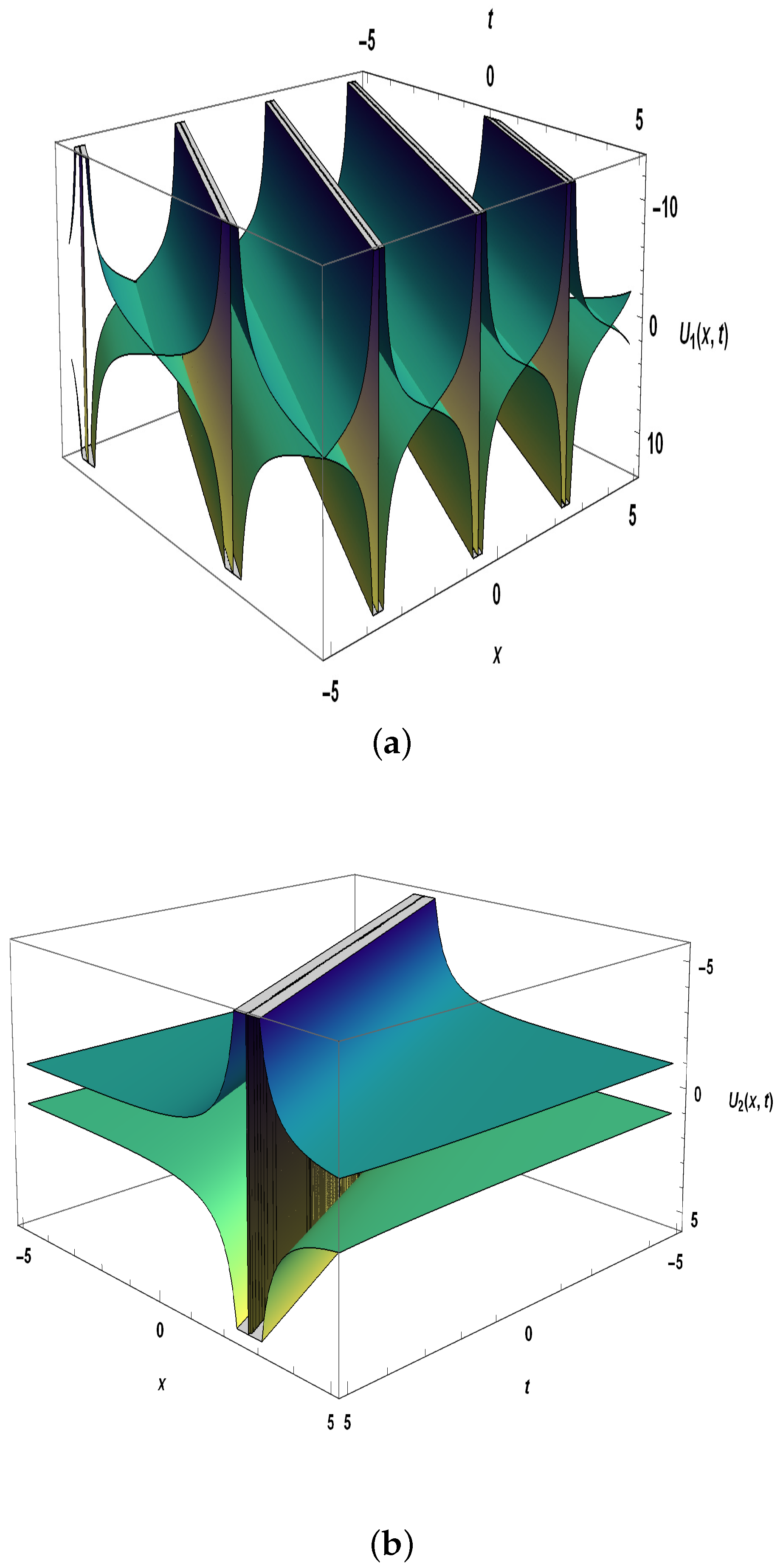
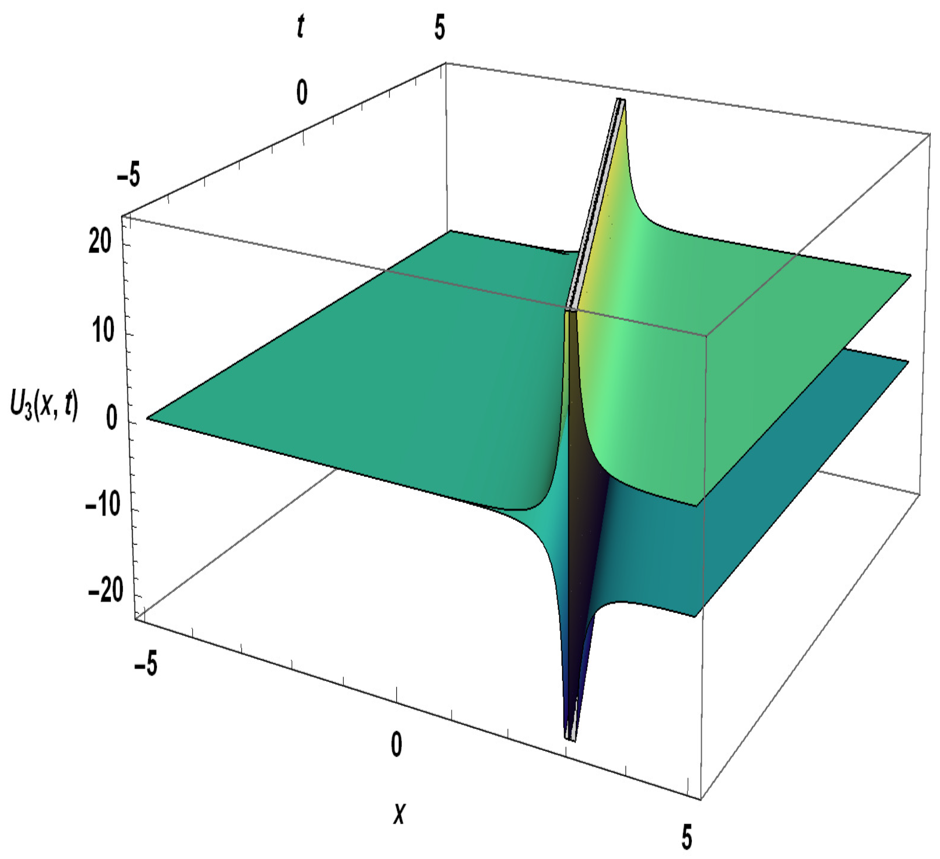
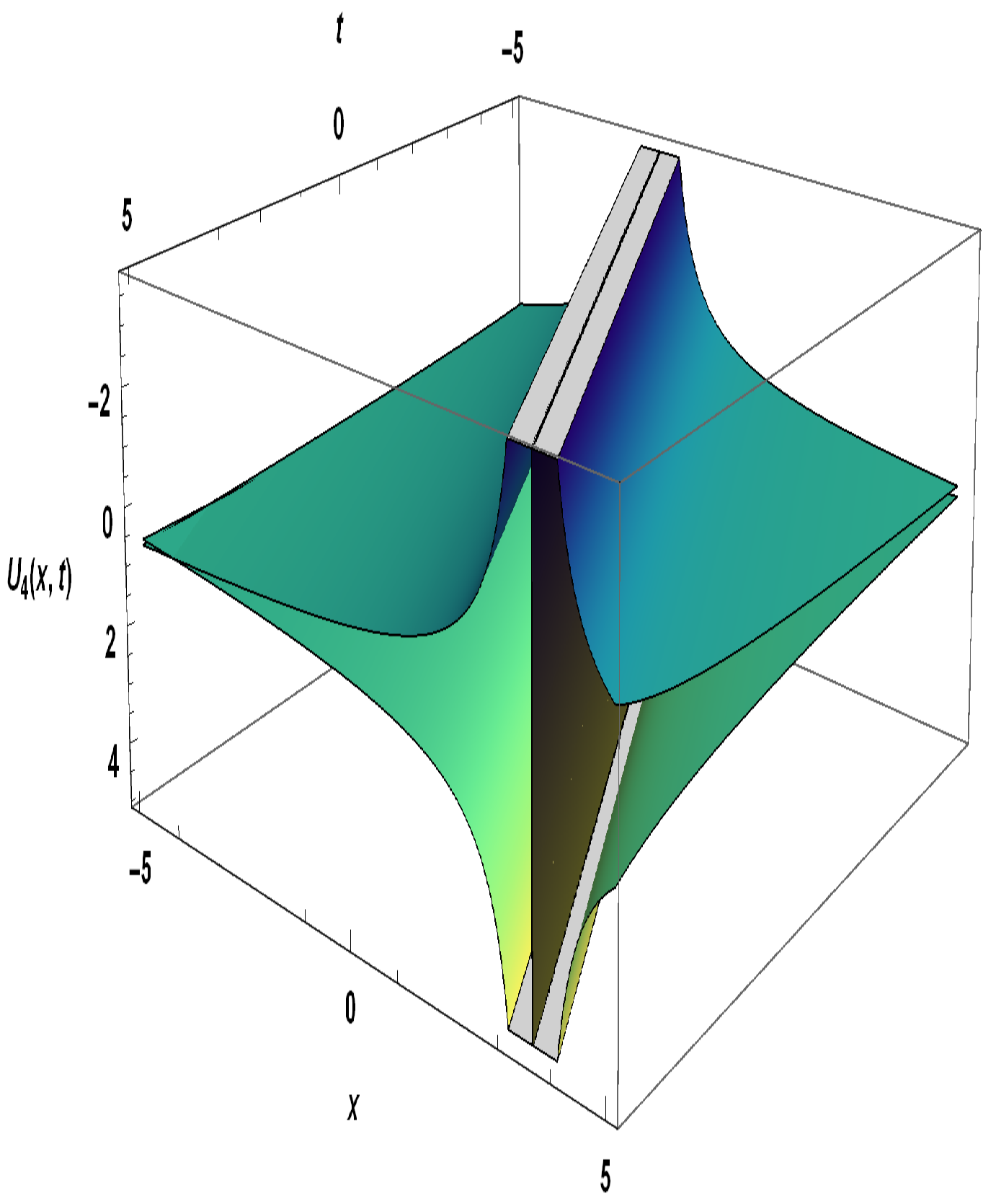
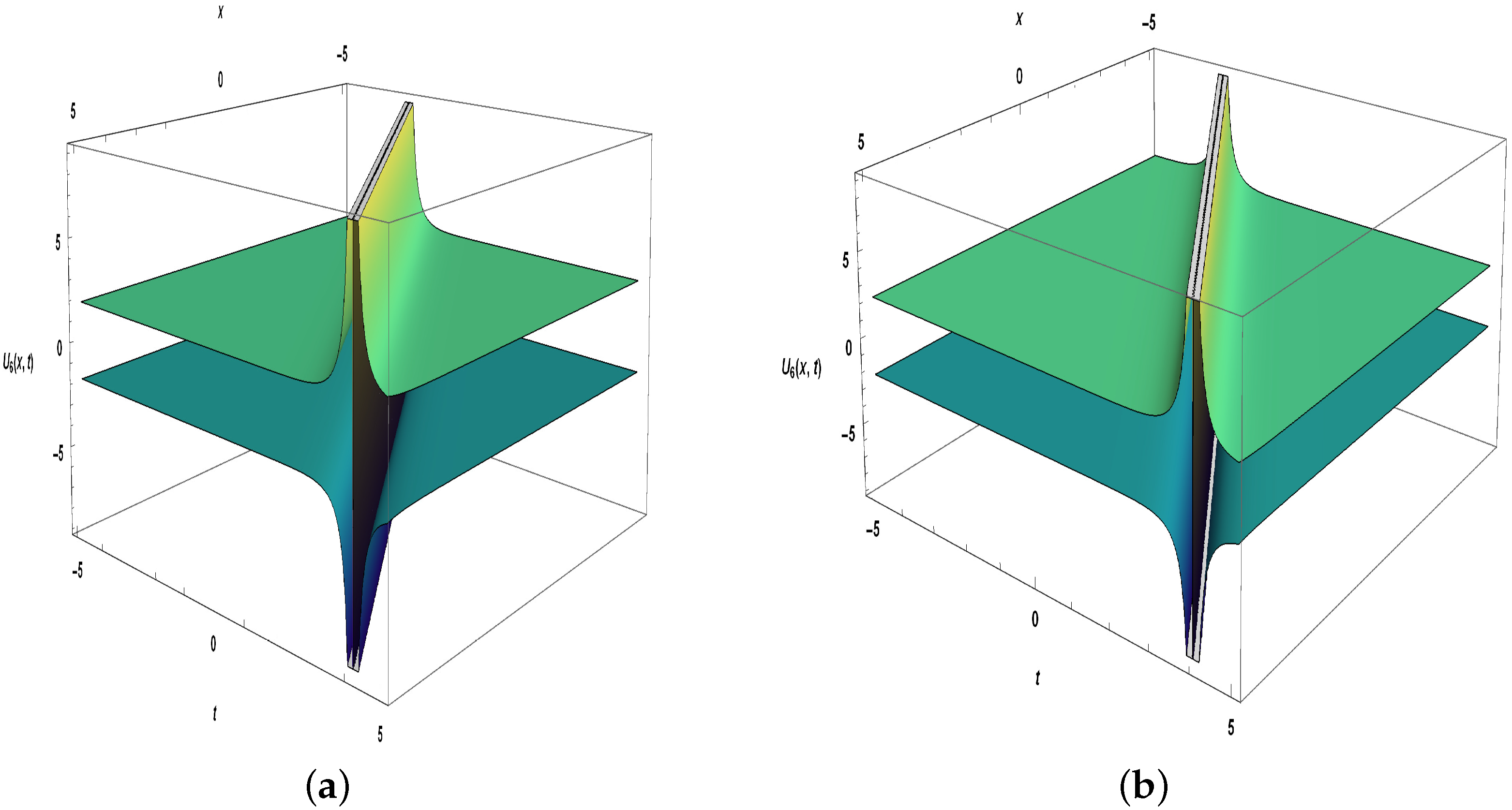
5. Extraction of Solitons from a Negative-Order KdV-CBS Equation

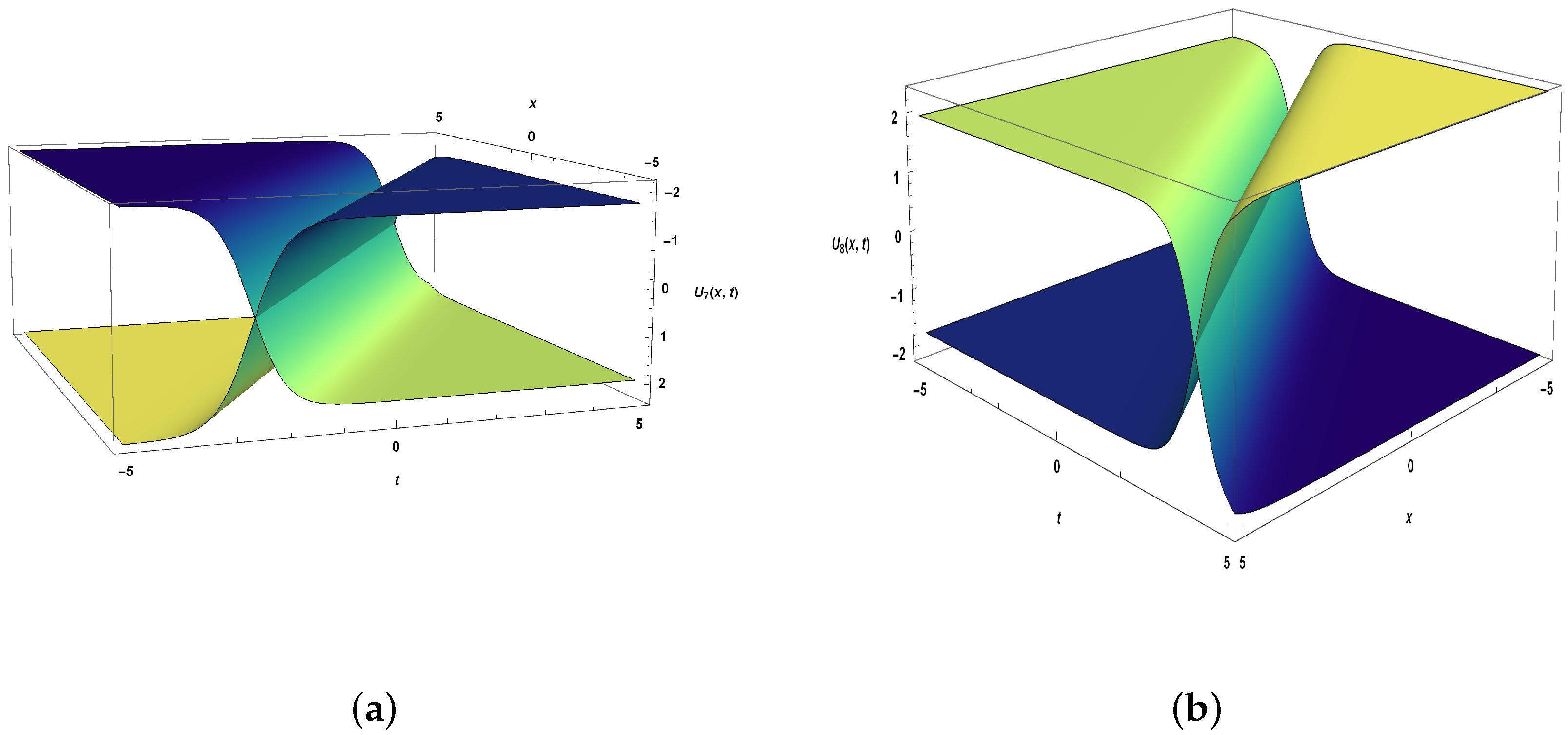
In this section, we find the optical solitary wave solutions for Equation (26) using the extended simple equation method (ESEM). Using this method, the initial solution takes the following form [44]:

$$\begin{array}{c}\hfill U\left(\xi \right)=\sum _{i=-N}^N{B}_i{\phi }^i\left(\xi \right),\end{array}$$

(27)

where $B_i(i=-N,-N+1,\cdots ,-1,0,1,\cdots ,N-1,N)$ are the unknown coefficients to be found and N is the positive integer which can be calculated using balance principle on Equation (26). By applying balance principle, we get $N=1$ and therefore, Equation (27) takes the form

$$\begin{array}{c}\hfill U\left(\xi \right)=\frac{B_{-1}}{\phi \left(\xi \right)}+B_0+B_1\phi \left(\xi \right),\end{array}$$

(28)

which satisfies the ansatz equation given by

$$\begin{array}{c}\hfill {\phi }^{\prime }\left(\xi \right)=b_0+b_1\phi \left(\xi \right)+b_2{\phi }^2\left(\xi \right),\end{array}$$

(29)

where $b_0,b_1$ and $b_2$ are arbitrary constants.

If we take $b_1=0$ in Equation (29), then the ansatz Equation (29) converts to Riccati equation, and we have

$$\begin{array}{c}\hfill \phi \left(\xi \right)=\frac{\sqrt{b_0{b}_2}}{b_2}tan\left(\sqrt{b_0{b}_2}(\xi +{\xi }_0)\right),b_0{b}_2>0,\end{array}$$

(30)

$$\begin{array}{c}\hfill \phi \left(\xi \right)=-\frac{\sqrt{-b_0{b}_2}}{b_2}tanh\left(\sqrt{-b_0{b}_2}\xi -\frac{mln\left({\xi }_0\right)}{2}\right),{\xi }_0>0,b_0{b}_2<0,m=\pm 1.\end{array}$$

(31)

If we take $b_0=0$ in Equation (29), then the ansatz Equation (29) becomes Bernoulli equation, and we have

$$\begin{array}{c}\hfill \phi \left(\xi \right)=\frac{b_1{e}^{b_1\xi }}{b_1{\xi }_0-b_2{e}^{b_1\xi }},b_1>0,\end{array}$$

(32)

$$\begin{array}{c}\hfill \phi \left(\xi \right)=-\frac{b_1{e}^{b_1\xi }}{b_1{\xi }_0+b_2{e}^{b_1\xi }},b_1<0.\end{array}$$

(33)

If we take $b_0=b_1=0$ in Equation (29), then the ansatz Equation (29) converts to sparable equation, and in this case we have

$$\begin{array}{c}\hfill \phi \left(\xi \right)=\frac{1}{-b_2\xi +{\xi }_0},b_2\ne 0.\end{array}$$

(34)

Thus, following is the general solution to ansatz Equation (29):

$$\begin{array}{c}\hfill \phi \left(\xi \right)=-\frac{b_1-\sqrt{4b_0{b}_2-b_1^2}tan\left(\frac{\sqrt{4b_0{b}_2-b_1^2}}{2}(\xi +{\xi }_0)\right)}{2b_2},4b_0{b}_2>b_1^2,b_2>0,\end{array}$$

(35)

$$\begin{array}{c}\hfill \phi \left(\xi \right)=\frac{b_1+\sqrt{4b_0{b}_2-b_1^2}tan\left(\frac{\sqrt{4b_0{b}_2-b_1^2}}{2}(\xi +{\xi }_0)\right)}{2b_2},4b_0{b}_2>b_1^2,b_2<0,\end{array}$$

(36)

where ${\tau }_0$ represents the constant of integration. Now, after putting Equation (28) along with Equation (29) into Equation (26) generates a system of algebraic equations and further doing some algebra calculations, we get the following cases:

• Case 1. When $b_1=0$,

$$\begin{array}{c}\hfill A_{-1}=\mp \frac{a-\lambda -cv-b\mu }{8b{b}_2},A_1=\mp 2b_2,b_0=\frac{\lambda +cv+b\mu -a}{16b_{2}b}.\end{array}$$

(37)

By using parameters defined in Equation (37) along with the corresponding ansatz equation yields the following solution

$$U_1\left(\xi \right)=\mp \frac{-a+\lambda +cv+b\mu +8A_{0}tan\left(\sqrt{b_0{b}_2}(\xi +{\xi }_0)\right)\sqrt{b_0{b}_2}b-16b_{2}tan{\left(\sqrt{b_0{b}_2}(\xi +{\xi }_0)\right)}^2{b}_{0}b}{8btan\left(\sqrt{b_0{b}_2}(\xi +{\xi }_0)\right)\sqrt{b_0{b}_2}},$$

(38)

$$U_2\left(\xi \right)=\mp \frac{2b_0{b}_2+A_0\sqrt{-b_0{b}_2}tanh\left(\frac{mln\left({\xi }_0\right)}{2}-\sqrt{-b_0{b}_2}\xi \right)+2b_2{b}_{0}tanh{\left(\frac{mln\left({\xi }_0\right)}{2}-\sqrt{-b_0{b}_2}\xi \right)}^2}{\sqrt{-b_0{b}_2}tanh\left(-\sqrt{-b_0{b}_2}\xi +\frac{mln\left({\xi }_0\right)}{2}\right)},$$

(39)

where $b_0=\frac{\lambda +cv+b\mu -a}{16b_{2}b}$, $\xi =x+by+cz-at$ and $m=\pm 1$ (Figure 1).

• Case 2. When $b_0=0$,

$$\begin{array}{c}\hfill A_{-1}=0,A_1=\mp 2b_2,b_1=\sqrt{\frac{a-b\mu -\lambda -cv}{b}}.\end{array}$$

(40)

By using paramors defined in Equation (40) along with the corresponding ansatz equation yields the following solution

$$\begin{array}{c}\hfill U_3\left(\xi \right)=\frac{A_0\sqrt{\frac{a-b\mu -\lambda -cv}{b}}{\xi }_0-\left(A_0{b}_2-A_1\sqrt{\frac{a-b\mu -\lambda -cv}{b}}\right)e^{\sqrt{\frac{a-b\mu -\lambda -cv}{b}}\xi }}{\sqrt{\frac{a-b\mu -\lambda -cv}{b}}{\xi }_0-b_2{e}^{\sqrt{\frac{a-b\mu -\lambda -cv}{b}}\xi }},b\ne 0;\end{array}$$

(41)

where $A_1=\mp 2b_2$ and $\xi =x+by+cz-at$ (Figure 2).

• Case 3. When $b_0=b_1=0$,

$$\begin{array}{c}\hfill A_{-1}=\mp \frac{a-\lambda -cv-b\mu }{6b_{2}b},A_1=\mp 2b_2.\end{array}$$

(42)

By using paramors defined in Equation (42) along with the corresponding ansatz equation yields the following solution

$$\begin{array}{c}\hfill U_4\left(\xi \right)=\frac{A_{-1}{b}_2^2{\xi }^2-2A_{-1}{b}_2\xi {\xi }_0+A_{-1}{\xi }_0^2-A_0{b}_2\xi +A_0{\xi }_0+A_1}{{\xi }_0-b_2\xi },\end{array}$$

(43)

where $A_{-1}=\mp \frac{a-\lambda -cv-b\mu }{6b_{2}b},A_1=\mp 2b_2$ and $\xi =x+by+cz-at$ (Figure 3).

• Case 4.

$$\begin{array}{cc}\hfill & \left(\mathbf{i}\right):A_{-1}=\frac{b{b}_1^2+\lambda +cv+b\mu -a}{2b_{2}b},A_1=0,b_0=\frac{b{b}_1^2+\lambda +cv+b\mu -a}{4b_{2}b};\hfill \\ & \left(\mathbf{ii}\right):A_{-1}=0,A_1=-2b_2,b_0=\frac{b{b}_1^2+\lambda +cv+b\mu -a}{4b_{2}b},b,b_2\ne 0.\hfill \end{array}$$

(44)

By using paramors defined in Equation (44) along with the corresponding anstaz equation yields the following solution

$$\begin{array}{c}\hfill U_5\left(\xi \right)=\frac{2A_{-1}{b}_2-A_0{b}_1+A_{0}tan\left(\frac{1}{2}\sqrt{\frac{\lambda +cv+b\mu -a}{b}}(\xi +{\xi }_0)\right)\sqrt{\frac{\lambda +cv+b\mu -a}{b}}}{-b_1+tan\left(\frac{1}{2}\sqrt{\frac{\lambda +cv+b\mu -a}{b}}(\xi +{\xi }_0)\right)\sqrt{\frac{\lambda +cv+b\mu -a}{b}}},4b_0{b}_2>b_1^2,b_2>0,\end{array}$$

(45)

$$\begin{array}{c}\hfill U_6\left(\xi \right)=\frac{2A_{-1}{b}_2+A_0{b}_1+A_{0}tan\left(\frac{1}{2}\sqrt{\frac{\lambda +cv+b\mu -a}{b}}(\xi +{\xi }_0)\right)\sqrt{\frac{\lambda +cv+b\mu -a}{b}}}{b_1+tan\left(\frac{1}{2}\sqrt{\frac{\lambda +cv+b\mu -a}{b}}(\xi +{\xi }_0)\right)\sqrt{\frac{\lambda +cv+b\mu -a}{b}}},4b_0{b}_2>b_1^2,b_2<0,\end{array}$$

(46)

and

$$\begin{array}{c}\hfill U_7\left(\xi \right)=\frac{2A_0{b}_2-A_1{b}_1+A_{1}tan\left(\frac{1}{2}\sqrt{\frac{\lambda +cv+b\mu -a}{b}}(\xi +{\xi }_0)\right)\sqrt{\frac{\lambda +cv+b\mu -a}{b}}}{2b_2},b_2>0,\end{array}$$

(47)

$$\begin{array}{c}\hfill U_8\left(\xi \right)=\frac{2A_0{b}_2+A_1{b}_1+A_{1}tan\left(\frac{1}{2}\sqrt{\frac{\lambda +cv+b\mu -a}{b}}(\xi +{\xi }_0)\right)\sqrt{\frac{\lambda +cv+b\mu -a}{b}}}{2b_2},b_2<0,\end{array}$$

(48)

where $A_{-1}=\mp \frac{a-b{b}_1^2-\lambda -cv-b\mu }{2b_{2}b},A_1=\mp 2b_2$ and $\xi =x+by+cz-at$ (Figure 4 and Figure 5).

6. Concluding Remarks

The present work has obtained several new results for the $(3+1)$ negative-order KdV-CBS equation. Firstly, Lie point symmetries and low-order conservation laws have been derived. From the translation symmetries, travelling wave reductions are obtained. Moreover, from the invariant conservation laws under translations two first integrals are obtained for the travelling wave ODE. It happens that these two first integrals are functionally independent and a triple reduction has been derived, yielding a first-order ODE. For some particular cases of the parameters, the general solution is obtained in terms of the Weierstrass function and a line-kink solution is obtained for the $(3+1)$ negative-order KdV-CBS Equation (1). These explicit invariant solutions can be expected to be important in understanding the asymptotics of more general solutions of (1).

Secondly, the extended simple equation approach has been used to obtain the exact solutions for the negative-order KdV-CBS equation, which is a powerful method to solve nonlinear PDEs. These solutions include solitary wave solutions, specifically singular and dark solitons. In addition, numerical solutions are represented in 3D plots as shown in Figure 1, Figure 2, Figure 3, Figure 4 and Figure 5 to provide physical meaning of nonlinear phenomena. These solutions could be highly useful in comprehending physical phenomena in several disciplines of applied mathematics.

References

1. Wazwaz, A.M. A new (2+ 1)-dimensional Korteweg-de Vries equation and its extension to a new (3+ 1)-dimensional Kadomtsev-Petviashvili equation. Phys. Scr. 2011, 84, 035010. [Google Scholar] [CrossRef]
2. Wazwaz, A.M. Abundant solutions of various physical features for the (2+ 1)-dimensional modified KdV-Calogero–Bogoyavlenskii–Schiff equation. Nonlinear Dyn. 2017, 89, 1727–1732. [Google Scholar] [CrossRef]
3. El-Kalaawy, O.H.; Ibrahim, R.S. Solitary Wave Solution of the Two-Dimensional Regularized Long-Wave and Davey-Stewartson Equations in Fluids and Plasmas. Appl. Math. 2012, 3, 833–843. [Google Scholar] [CrossRef]
4. Al-Amr, M.O. New applications of reduced differential transform method. Alex. Eng. J. 2014, 53, 243–247. [Google Scholar] [CrossRef]
5. Helal, M.A.; Seadawy, A.R. Variational method for the derivative nonlinear Schrödinger equation with computational applications. Phys. Scr. 2009, 80, 350–360. [Google Scholar] [CrossRef]
6. Salman, F.; Raza, N.; Basendwah, G.A.; Jaradat, M.M. Optical solitons and qualitative analysis of nonlinear Schrodinger equation in the presence of self steepening and self frequency shift. Results Phys. 2022, 39, 105753. [Google Scholar] [CrossRef]
7. Jhangeer, A.; Raza, N.; Rezazadeh, H.; Seadawy, A. Nonlinear self-adjointness, conserved quantities, bifurcation analysis and travelling wave solutions of a family of long-wave unstable lubrication model. Pramana 2020, 94, 1–9. [Google Scholar] [CrossRef]
8. Taghizadeh, N.; Mirzazadeh, M. The modified extended tanh method with the Riccati equation for solving nonlinear partial differential equations. Math. Aeterna 2012, 2, 145–153. [Google Scholar]
9. Cheemaa, N.; Chen, S.; Seadawy, A.R. Propagation of isolated waves of coupled nonlinear (2+ 1)-dimensional Maccari system in plasma physics. Results Phys. 2020, 17, 102987. [Google Scholar] [CrossRef]
10. Lu, D.; Seadawy, A. R.; Iqbal, M. Mathematical methods via construction of traveling and solitary wave solutions of three coupled system of nonlinear partial differential equations and their applications. Results Phys. 2018, 11, 1161–1171. [Google Scholar] [CrossRef]
11. Yang, X.F.; Deng, Z.C.; Wei, Y. A Riccati-Bernoulli sub-ODE method for nonlinear partial differential equations and its application. Adv. Differ. Equ. 2015, 2015, 1–17. [Google Scholar] [CrossRef] [Green Version]
12. Jiong, S. Auxiliary equation method for solving nonlinear partial differential equations. Phys. Lett. A 2003, 309, 387–396. [Google Scholar]
13. Zhang, H. New application of the (G′/G)-expansion method. Commun. Nonlinear Sci. Numer. Simul. 2009, 14, 3220–3225. [Google Scholar] [CrossRef]
14. Liao, S. Comparison between the homotopy analysis method and homotopy perturbation method. Appl. Math. Comput. 2005, 169, 1186–1194. [Google Scholar] [CrossRef]
15. Raza, N.; Rafiq, M.H.; Kaplan, M.; Kumar, S.; Chu, Y. The unified method for abundant soliton solutions of local time fractional nonlinear evolution equations. Results Phys. 2021, 22, 103979. [Google Scholar] [CrossRef]
16. Wazwaz, A.M.; Osman, M.S. Analyzing the combined multi-waves polynomial solutions in a two-layer-liquid medium. Comput. Math. Appl. 2018, 76, 276–283. [Google Scholar] [CrossRef]
17. Javid, A.; Raza, N. Singular and dark optical solitons to the well posed Lakshamanan-Porsezian-Daniel model. Optik 2018, 171, 120–129. [Google Scholar] [CrossRef]
18. Ekici, M.; Sonmezoglu, A.; Zhou, Q.; Biswas, A.; Ullah, M.Z.; Asma, M.; Moshokoa, S.P.; Belic, M. Optical solitons in DWDM system by extended trial equation method. Optik 2017, 141, 157–167. [Google Scholar] [CrossRef]
19. Wang, M.L.; Zhou, Y.B.; Li, Z.B. Application of homogeneous balance method to exact solutions of nonlinear equations in mathematical physics. Phys. Lett. A 1996, 216, 67–75. [Google Scholar] [CrossRef]
20. Vahidi, J.; Zabihi, A.; Rezazadeh, H.; Ansari, R. New extended direct algebraic method for the resonant nonlinear Schrödinger equation with Kerr law nonlinearity. Optik 2021, 227, 165936. [Google Scholar] [CrossRef]
21. Arshad, M.; Seadawy, A.R.; Lu, D. Optical soliton solutions of the generalized higher-order nonlinear Schrödinger equations and their applications. Opt. Quantum Electron. 2018, 5, 1–6. [Google Scholar] [CrossRef]
22. Alhussain, Z.A.; Raza, N. New Optical Solitons with Variational Principle and Collective Variable Strategy for Cold Bosons in Zig-Zag Optical Lattices. J. Math. 2022, 2022. [Google Scholar] [CrossRef]
23. Kumar, M.; Kumar, R.; Kumar, A. On similarity solutions of Zabolotskaya-Khokhlov equation. Comput. Math. Appl. 2014, 68, 454–463. [Google Scholar] [CrossRef]
24. Ray, S.S. Lie symmetry analysis and reduction for exact solution of (2+ 1)-dimensional Bogoyavlensky-Konopelchenko equation by geometric approach. Mod. Phys. Lett. B 2018, 32, 1850127. [Google Scholar] [CrossRef]
25. Vinita; Ray, S.S. Optical soliton group invariant solutions by optimal system of Lie subalgebra with conservation laws of the resonance nonlinear Schrödinger equation. Mod. Phys. Lett. B 2020, 34, 2050402. [Google Scholar] [CrossRef]
26. Wazwaz, A.M. Exact solutions of compact and noncompact structures for the KP-BBM equation. Appl. Math. Comput. 2005, 169, 700–712. [Google Scholar] [CrossRef]
27. Olver, P.J. Application of Lie Groups to Differential Equations; Springer: NewYork, NY, USA, 1993. [Google Scholar]
28. Kumar, S.; Kumar, D.; Wazwaz, A.M. Group invariant solutions of (3+ 1)-dimensional generalized B-type Kadomstsev Petviashvili equation using optimal system of Lie subalgebra. Phys. Scr. 2019, 94, 065204. [Google Scholar] [CrossRef]
29. Bai, Y.; Bilige, S.; Chaolu, T. Potential symmetries, one-dimensional optimal system and invariant solutions of the coupled Burgers? equations. J. Appl. Math. Phys. 2018, 6, 1825. [Google Scholar] [CrossRef]
30. Kara, A.H.; Biswas, A.; Zhou, Q.; Moraru, L.; Moshokoa, S.P.; Belic, M. Conservation laws for optical solitons with Chen?Lee?Liu equation. Optik 2018, 174, 195–198. [Google Scholar] [CrossRef]
31. Jafari, H.; Kadkhoda, N.; Azadi, M.; Yaghobi, M. Group classification of the time-fractional Kaup-Kupershmidt equation. Sci. Iran. 2017, 24, 302–307. [Google Scholar] [CrossRef]
32. Kadkhoda, N.; Jafari, H.; Moremedi, G.M.; Baleanu, D.; Qaenat, I.R.; Babolsar, I.R. Optimal system and symmetry reduction of the (1+ 1) dimensional Sawada–Kotera equation. Int. J. Pure Appl. Math. 2016, 103, 215–226. [Google Scholar] [CrossRef]
33. Wazwaz, A.M. Two new Painlevé integrable KdV-Calogero–Bogoyavlenskii–Schiff (KdV-CBS) equation and new negative-order KdV-CBS equation. Nonlinear Dyn. 2021, 104, 4311–4315. [Google Scholar] [CrossRef]
34. Anco, S.C.; Gandarias, M. Symmetry multi-reduction method for partial differential equations with conservation laws. Commun. Nonlin. Sci. Numer. Simul. 2020, 91, 105349. [Google Scholar] [CrossRef]
35. Olver, P.J. Applications of Lie Groups to Differential Equations; Springer: Berlin/Heidelberg, Germany, 1986. [Google Scholar]
36. Bluman, G.W.; Cheviakov, A.; Anco, S.C. Applications of Symmetry Methods to Partial Differential Equations; Springer: New York, NY, USA, 2009. [Google Scholar]
37. Anco, S.C. Generalization of Noether’s theorem in modern form to non-variational partial differential equations. In Recent Progress and Modern Challenges in Applied Mathematics, Modeling and Computational Science; Springer: New York, NY, USA, 2017; pp. 119–182. [Google Scholar]
38. Anco, S.C.; Gandarias, M.L.; Recio, E. Line-solitons, line-shocks, and conservation laws of a universal KP-like equation in 2+1 dimensions. J. Math. Anal. Appl. 2021, 504, 125319. [Google Scholar] [CrossRef]
39. Sjöberg, A. Double reduction of PDEs from the association of symmetries with conservation laws with applications. Appl. Math. Comput. 2007, 184, 608–616. [Google Scholar] [CrossRef]
40. Sjöberg, A. On double reduction from symmetries and conservation laws. Nonlin. Analysis Real World Appl. 2009, 10, 3472–3477. [Google Scholar] [CrossRef]
41. Bokhari, A.H.; Dweik, A.Y.; Zaman, F.D.; Kara, A.H.; Mahomed, F.M. Generalization of the double reduction theory. Nonlin. Analysis Real World Appl. 2010, 11, 3763–3769. [Google Scholar] [CrossRef]
42. Whittaker, E.E.; Watson, G.M. Modern Analysis, 4th ed.; Cambridge University Press: Cambridge, UK, 1927. [Google Scholar]
43. Abramowitz, M.; Stegun, I.A. Handbook of Mathematical Tables; Dover: New York, NY, USA, 1965. [Google Scholar]
44. Lu, D.; Seadawy, A.; Arshad, M. Applications of extended simple equation method on unstable nonlinear Schrödinger equations. Optik 2017, 140, 136–144. [Google Scholar] [CrossRef]
Figure 1. Graphical representation of Equations (38) and (39) with suitable parameters b = 0.2 , c = 0.1 , v = 0.4 , λ = 0.1 , μ = 1 , A 0 = 0.1 , ξ 0 = 1 , m = 1 , y = 0 , z = 0 : (a) a = 0.5 , b 2 = 0.2 (b) a = 0.5 , b 2 = 0.2 .
Symmetry 14 01861 g001
Figure 2. Graphical representation of Equation (41) with suitable parameters b = 0.1 , c = 0.3 , v = 1.2 , λ = 0.1 , μ = 1 , A 0 = 0.1 , ξ 0 = 1 , m = 1 , y = 0 , z = 0 , a = 0.4 , b 2 = 0.2 .
Symmetry 14 01861 g002
Figure 3. Graphical representation of Equation (43) with suitable parameters a = 0.5 , b = 0.1 , c = 0.1 , v = 0.2 , λ = 0.4 , μ = 1 , A 0 = 0.6 , ξ 0 = 1 , b 2 = 1 , m = 1 , y = 0 , z = .
Symmetry 14 01861 g003
Figure 4. Graphical representation of Equations (45) and (46) with suitable parameters a = 1.5 , b = 0.2 , c = 0.2 , v = 0.3 , λ = 0.4 , μ = 1 , A 0 = 0.1 , ξ 0 = 1 , b 1 = 0.2 , m = 1 , y = 0 , z = 0 : (a) b 2 = 0.2 (b) b 2 = 0.2 .
Symmetry 14 01861 g004
Figure 5. Graphical representation of Equations (47) and (48) with suitable parameters a = 1.5 , b = 0.2 , c = 0.2 , v = 0.3 , λ = 0.4 , μ = 1 , A 0 = 0.1 , ξ 0 = 1 , b 1 = 0.2 , m = 1 , y = 0 , z = 0 : (a) b 2 = 0.2 (b) b 2 = 0.2 .
Symmetry 14 01861 g005
Publisher’s Note: MDPI stays neutral with regard to jurisdictional claims in published maps and institutional affiliations.