Abstract
The 1992 Cairo earthquake, with a moment magnitude of 5.8, is the most catastrophic earthquake to shock the Greater Cairo (GC) in recent decades. According to the very limited number of seismological stations at that time, the peak ground acceleration (PGA) caused by this event was not recorded. PGA calculation requires identification of nature of the earthquake source, the geologic setting of the path between the source and site under investigation and soil dynamic properties of the site. Soil dynamic properties are acquired by geotechnical investigations and/or geophysical survey. These two methods are costly and are not applicable in regional studies. This study presents an adaptive and reliable PGA prediction model using machine learning (ML) along with six standard geographic information system (GIS) interpolation methods (IDW, Kriging, Natural, Spline, TopoToR, and Trend) to predict the spatial distribution of PGA caused by this event over the GC. The model is employed to estimate the exposure of the urban area and population in the GC based on the available geotechnical and geophysical investigations. The exposure (population) data is from free and easy-access sources, e.g., Landsat images and the Global Human Settlement Population Grid (GHS-POP). The results show that Natural, Spline, and Trend are not suitable GIS interpolation techniques for generating seismic hazard maps (SHMs), while the Kriging Method shows sufficient prediction. Interestingly, with an accuracy of 96%, the ML model outperforms the classical GIS methodologies.
1. Introduction
Natural disasters are the most common problem that human settlements, particularly in megacities throughout the globe, have to deal with [1]. Natural catastrophes pose a significant threat to mega-cities as well. According to statistics published by the UN (United Habitat’s Nations Human Settlements Programme), all megacities are prone to natural disasters varying from geological (earthquake ground shaking and mass movements) to meteorological (flash flooding and storms), extreme weather events (extreme heat and cold) and wildfires, indicating the need to develop different risk reduction strategies for various conditions in megacities [2]. Earthquakes have the potential to create liquefaction, landslides, fires, and tsunamis, all of which would result in a much greater amount of damage and losses [3].
Seismic hazard maps (SHMs) represent the regional distribution of the hazard caused by the earthquake’s ground motion in an area. So, seismic intensity parameters such as peak ground acceleration (PGA) and peak ground velocity (PGV) are usually used as hazard indications in conventional SHMs. Many SHMs have been proposed and developed around the world [4]. SHMs are usually used by planners, engineers, and developers to save lives and money [5]. They are also used in building codes, seismic risk assessment, and disaster management. Tsunamis, landslides, and liquefaction are all possible secondary effects of earthquakes. Therefore, gathering SHMs with other information compiled from the tectonic maps, geological, geodetic, and geophysical data sets can be used to identify the potential sites of these effects. Kim et al. (2020) used the GIS interpolation methodologies to map the soil classification and to produce SHMs based on remote sensing and geotechnical information in Deajeon, South Korea. At the end of their study [6], Kim et al. (2020) approved the applicability of using GIS interpolation methodologies in producing SHMs and strongly recommended the integration of the remote sensing-based and in situ geotechnical information in producing seismic zonation maps [6].
The excessive placement of major cities around the world, expansion in urbanization and population, and growing income all contribute to increasing the exposure in hazard-prone regions [7]. Therefore, urban planning based on reliable hazard maps is necessary to safeguard inhabitants from the consequences of natural disasters [8,9]. Producing SHMs based on the earthquake scenario approach requires knowledge about the faulting mechanism, earthquake source parameters, the crustal structure between the earthquake source and the site under investigation and the soil dynamic properties in the site under investigation. Earthquake faulting mechanism and earthquake source parameters can be inferred directly from the digital earthquake record. The nature of the crustal structure can be found in the previous geophysical and seismological studies. However, the dynamic properties of the soil at the site of interest are obtained from the in situ geotechnical boreholes and/or geophysical measurements. In situ geotechnical boreholes and/or geophysical investigations are costly, time-consuming and not applicable for regional studies. Therefore, producing regional scale SHMs considering the local site conditions is a great challenge, as the main obstacle is the limited number of available geotechnical data and geophysical measurements. Consequently, implementing new approaches using recent methodologies (i.e., remote sensing, GIS and machine learning (ML)) based on free and easy-access data to overcome the data limits and deficiency of the traditional techniques is a very important quick and low-cost solution.
Remote sensing technology has been advanced dramatically in the last decade, providing the opportunity for more precise characterization of urban monitoring [10]. Remote sensing data has several benefits and plays an important role in the inventory evaluation and monitoring of environmental assets based on spatial data; hence, use of this technology in a wide range of industries increases [11,12]. However, remote sensing applications are found to be crucial for third-world nations since it is difficult for governments to update their databases using standard methods due to the time and expense connected with them. Remote sensing data may also be used to determine land use in urban areas [13]. There is a large amount of satellite imagery data coming, for example, from Landsat, IKONOS-2, and OrbView-3. However, Landsat has been selected as the best choice for monitoring spatial details, given the availability of spectral satellite data with reasonably long timespans and suitable accuracy [14]. Landsat data are free and easy-access data which are available and easy to download from the United States Geological Survey website [15]; these types of data may provide main findings that are near to real-life situations [16].
The Joint Research Centre (JRC) has just published the most recent worldwide gridded population dataset, dubbed the Global Human Settlement Population Grid (GHS-POP) [17]. Using this geographic raster dataset, you could see the population of the city, given as the number of people per cell, published in 2018 [18,19]. These estimations were taken from the CIESIN GPWv4.10 datasets and dispersed from censuses or administrative units to grid cells based on the distribution and density of built-up areas as depicted in the Global Human Settlement Layer (GHSL) total world layer per epoch [18]. Global population raster maps are crucial for a variety of policy-making evaluations (from environmental assessment through disaster risk studies to city planning and management) [20]. As a result, accurate and up-to-date statistics on the population are critical. Simple GIS statistics and analyses are used to ensure the correctness of the collected data. The GHS-POP statistics are very reliable and independent of the study topic, according to the error values [21].
The geographic information system (GIS) commonly stores spatial data as discrete points or splits data in its spatial database. For this reason, it is preferable to conduct a survey of all geographic area data samples and then end the attribute value sample to gather comprehensive geographic data. According to some studies, this is a waste of time and money [22,23]. GIS spatial interpolation methods provide an effective way of predicting the proper geographic distribution of data, enhancing data density, acquiring full information for missing data, and establishing an intense distribution of data with a small observational data set. Spatial interpolation is a way of making informed assumptions that incorporate both the investigator and the GIS when the value of a continuous field has not been measured at a specific place [22].
Machine learning (ML) algorithms have recently emerged to tackle many research problems [24,25]. This started with the success of the use of convolutional neural networks (CNNs) for image recognition. This, in turn, has raised the interest in applying other ML algorithms to address a wide range of challenging research problems. ML tools can be used to build (learn) very complex relational models that classical approaches might not be able to capture given their models’ restrictions [26]. The application of ML tools has witnessed great success in addressing many challenging research problems, ranging from recommendation systems to autonomous driving cars [27]. In this regard, ML has proved beneficial in both classification and regression problems in calculating the ground motion parameters that are directly employed in seismic hazard and human safety [28,29,30]. Moreover, it can be utilized for creating effective seismic zonation maps [31].
The Greater Cairo (GC) region is one of the most densely populated locations in the world (about 13 million capita), with densely populated suburbs. Historical and recent earthquake catalogs prove that this mega city has experienced severe earthquakes that have destroyed many historical and archaeological structures [32,33]. The Dahshour seismic source is the seismic source that generates the most catastrophic earthquakes affecting the GC. On 12 October 1992, the Dahshour seismic source generated the most significant natural hazard in this region in more than a decade, causing a disproportionate amount of destruction and the loss of numerous lives [34] in the GC region, the Nile Valley, and the Nile Delta [35]. This significant event caused 561 deaths and left 9832 injured; more than 20,000 people were made homeless, and more than 8000 structures were damaged or destroyed; 50,000 people were displaced in the Cairo region alone, and the region was left with a damage bill of more than USD 35 million [36]. The study of the recent impact of such an event is very important for urban planning, seismic risk assessment, seismic risk reduction, and disaster management. The purpose of this research is threefold. For our first goal, the paper compares six GIS interpolation methods, in addition to the suggested ML method, in order to give recommendations for the most accurate method that will be used to predict PGA values and create SHMs. The second goal is to determine the contribution of using free and easy-access data sources for estimating the exposed urban area and population. The final goal is to examine the urban area’s exposure to the shaking caused by the 12 October 1992 Dahshour earthquake in GC using all tested interpolation methods and free and easy-access data sources.
2. Case Study and Materials
The Greater Cairo (GC) region, which is considered a mega city, has experienced severe historical earthquakes that have destroyed many historical and archaeological structures, e.g., the 7th of August 1847 earthquake [32,33]. This earthquake was generated in the Dahshour seismic source and caused a considerable loss of life and damage to the environment, infrastructures, and the national economy. On 12 October 1992, another significant earthquake originating in the Dahshour seismic source shocked Cairo. It is the most significant natural hazard to strike this region in more than a decade, causing a disproportionate amount of destruction and the loss of numerous lives [34] in the GC region, the Nile Valley, and the Nile Delta [35]. This significant event caused 561 deaths and left 9832 injured, while more than 20,000 people were made homeless, more than 8000 structures were damaged or destroyed, 50,000 people, were displaced in the Cairo region alone, and the region was left with a damage bill of more than USD 35 million [36]. Badawy et al. (2016) estimated the direct economic losses, in terms of building damage, which may be caused by an earthquake similar to the October 1992 earthquake to be USD 49.3 billion [37]. The study of the impact of such an event is very important because, as A. M. S. Mohamed et al. (2014) mentioned, the probability of the occurrence of an earthquake with ML = 5.0 is 99.9% in 100 years and 100% in 200 years in the Dahshour seismic source [38]. Therefore, producing seismic hazard maps (SHMs) of such significant events is very important for urban planning, seismic risk assessment, seismic risk reduction, and disaster management.
The current study has been performed after a very careful review and examination of the earthquake catalog compiled by [39]. Abdalzaher et al. (2020) compiled an earthquake catalog for Egypt and its surroundings. The earthquake catalog includes historical and instrumental events. Special attention is given to the earthquakes occurring around the GC. The impact of these events are studied and reviewed in the available publications and reports [39].
Egypt has 29 governorates where it included more than 70 villages and towns [40]. The most important of these is Cairo, Egypt’s capital. Greater Cairo includes the governorates of Cairo and Giza, as well as several districts from the Qalyubia Governorate, such as Shubra El Kheima and Obour [41,42]. This area is home to almost 20% of Egypt’s population [43,44]. As shown in Figure 1, a large portion of the GC comprises both exceptionally productive and arid desert territory around the Nile River [45,46]. GC is situated at 30°06′ north and 31°28′ east. Main agglomeration, New Urban Communities (NUC), and Peri-urban areas make up this region (PUA). PUAs are located in the north and west of the major agglomeration [47,48]. There are several different types of urban regions in the GC, including formal and informal slums, high- and low-class residential communities, and a variety of sized central business districts. Moreover, one-third of the GC’s urban mass is made up of illegal and informal slums, and 81 percent of these areas are located on private agricultural property [46]. Unplanned places are clearly the most hazardous, since their population are exposed to significant threats such as natural catastrophes, including earthquakes and landslides. Moreover, 61,000 people live in dangerous places in the GC (study area), according to Slum Development Fund 2012 inventory [45].
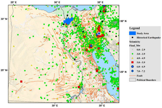
Figure 1.
Greater Cairo’s location in Egypt.
This part of the research provides the methodologies for reaching the main objectives of the article. The approach has been divided into five sections and will be explained in detail, but in the beginning, the data sources used in the methodology will be provided in Table 1.

Table 1.
Summary of used data sources.
3. Methodology
3.1. Create a Seismic Hazard Map (PGA)
PGA is the amplitude of the largest absolute acceleration recorded by an accelerometer at a site during an earthquake [49]. PGA is an important parameter for earthquake engineering, and the design basis for earthquakes is often defined in terms of PGA. In the current study, the scenario-based seismic hazard approach is implemented to estimate the ground motion parameters of Oct. 1992 earthquake. This approach is widely used in seismic risk assessment. The scenario based seismic hazard approach requires the definition of the characteristics of the seismic source, the nature of the path between the seismic source and the site of interest, and the local site condition expressed in the average shear wave velocity in the upper 30 m of the soil (Vs30). These inputs are implemented in a deterministic manner to predict the ground motion parameters at different sites in GC. The estimation/prediction of the PGA requires the definition of the seismic source, the nature of the path between the seismic source and the site of interest, and the local site condition expressed in the average shear wave velocity in the upper 30 m of the soil (Vs30). The Dahshour seismic source is the source, which generates the most hazardous earthquakes affecting GC. Many authors have defined the geometry of the Dahshour seismic source (e.g., [50,51,52]). Mohamed et al. (2012) used both historical and instrumental earthquake catalogues in addition to the geological and geophysical data to define the geometry of the Dahshour seismic source. This defined seismic source has been used in several seismic hazard studies in Egypt (e.g., [37,52,53,54]). In the current study, we use the Dahshour seismic source based on the definition of Mohamed et al. (2012).
The second required input is the nature of the path bath between the seismic source and the site of interest. Mainly, it depends on the geologic and tectonic settings of the path between the seismic source and the sites of interest, and it has a great impact on the shaking level. Therefore, it should be estimated in a proper way. In the current study, this parameter is expressed by using the Abrahmson and Silva (2014) ground motion prediction equation (GMPE) [55]. This equation is recommended by Ghareeb (2018) [56] as this study used the earthquake data recorded by the Egyptian National Seismological Network to select the proper equation that can be used in seismic hazard studies in Egypt. This GMPE has been used by [39,57] in estimating the seismic hazard of northern Egypt.
The velocity of the shear waves in the upper 30 m of the soil is considered a very important parameter used in predicting the ground motion caused by a certain earthquake. Vs30 can be measured directly in the field using different seismic methods. If directly measured Vs30 is not available, it can be estimated from the available geological and geotechnical data sets. The geologic setting of GC showing that the surface soil is a result of sedimentation from the River Nile. The basin, from which these deposits are formed, belongs to relatively old formations eroded by streams and rainfall [58]. Geologically, GC can be divided into three regions: the cultivated valley, the eastern, and the western sides of the Nile. The cultivated valley is the narrow strip that is penetrated longitudinally by the River Nile, made up of the thick uppermost sedimentary layers overlying the Pliocene deposits [59,60].
The geotechnical data is compiled from borehole data, shallow seismic refraction profiles, and micro-tremors arrays. In total, 600 boreholes are collected by the General Authority of Educational Buildings and provided to NRIAG for research. The geotechnical logs contain the site name, coordinates, water table depth, surface ground levels, stress foundation level, salt concentrations, soil type, thickness of each layer, grain size distribution parameters, plastic parameters, shear resistance parameters, including the N values for sand soils, consolidation parameters, swelling parameters, and collapse parameters. In order to make use of the essential shallow boreholes encountered in the dataset, the average count over the depth to the lowest recorded SPT-value N′ (d) was related to N’ (30). This step is performed using the statistical approach proposed by [61], considering (1). Then, the Vs30 is calculated as a function of N using the equation proposed by Iami and Tonochi (1982) [62].
Eleven shallow seismic profiles were acquired by [63]. These profiles were acquired in the southern part of Cairo in the areas occupied by the recent alluvium deposits and the Eocene limestone. Toni (2012) measured the velocity of the body waves (Vp) and the velocity of the shear waves (Vs) for each profile. Additionally, Toni, (2012) acquired three micro-tremor arrays in southern Cairo [63]. The Vs30 is directly measured in the field. The obtained and compiled Vs30 values have been used to produce a soil classification map for GC. This classification has been performed based on the National Earthquake Hazard Program [61]. As a result, the soil of GC is classified into four site classes, B, C, D, and E. The eastern part of GC is occupied by the Eocene limestone. The soil type is characterized by the high shear wave velocity. On the other hand, the soil class C is represented at the transition zone between the Eocene limestone and the alluvium deposits of the Nile River. The soil class D is dominating the alluvium deposits of the Nile River, and it reflects the very low Vs30, but the soil class E is represented by three small spots located at the Nile Deposits.
In the current study, the calculated PGA values are classified using the scale obtained by the United States Geological Survey (USGS) through the National Earthquake Hazard Program [61]. The USGS has established relationships between the observed or calculated PGA values and the intensity scales similar to the Mercalli scale. This scale correlates between the PGA values, certain levels of perceived shaking and the potential damage. This classification is widely used in producing shake maps. After classifying the calculated PGA values according to the USGS scheme, we found that GC has been exposed to three levels of shaking: moderate shaking on the eastern side, strong shaking in the middle part, and violent shaking in the narrow strip close to the Nile River.
3.2. Landsat Classification
Image categorization entails converting multiband raster images into a single-band raster with a number of classification groups that correspond to various kinds of land cover [64]. There are two major approaches to categorize a multi-band raster image: supervised and unsupervised classification. The supervised classification approach uses spectral signatures from training polygons that represent separate sample regions of the various land cover classes to classify images. The image analyzer collects these samples in order to categories the picture. With the unsupervised classification approach, the software discovers the spectral classes in the multi-band image without the analyst’s involvement, thereby becoming unsupervised. Identifying what the cluster symbolizes (e.g., water, desert, or water) is the next step once the clusters are discovered [64].
In order to confirm that the classified Landsat imagery is accurate, the Kappa coefficient [65] is one of the most often used techniques for measuring the amount of agreement across datasets to verifying the accuracy of supervised classification [66,67]. Ground truth points are used to produce random points that are compared against classified points in the confusion matrix to determine how accurate a classified map is. Google Earth is often used to evaluate ground truth points because imagery at these resolutions enables viewers to easily differentiate between main natural land cover classes and to detect components of the developed environment, such as individual residences, industrial buildings, and highways [68,69,70]. Using an overall Kappa index of agreement [71], both the user and the provider may be assessed for their correctness in each class. These ratings are shown on a scale from 0 to 1, with 1 being the maximum degree of accuracy [72].
3.3. Identifying Population
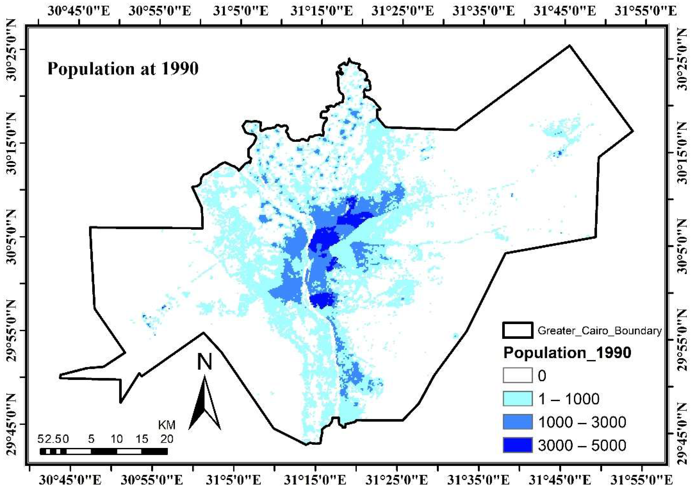
In this article, we use the GHS-POP data set as a valid open-source data source to analyze the amount of the population exposed to seismic hazard. This data set provides the spatial distribution of the population for all of the world, and we use the case study area’s boundary as a splitter to extract only the population distribution for GC, which is the focus of this article. Figure 2 depicts the final raster map for population, in which each cell value corresponds to the number of people living in that cell. In order to make it easier to study and comprehend, the map has been categorized into six different classes, as seen in Figure 2.
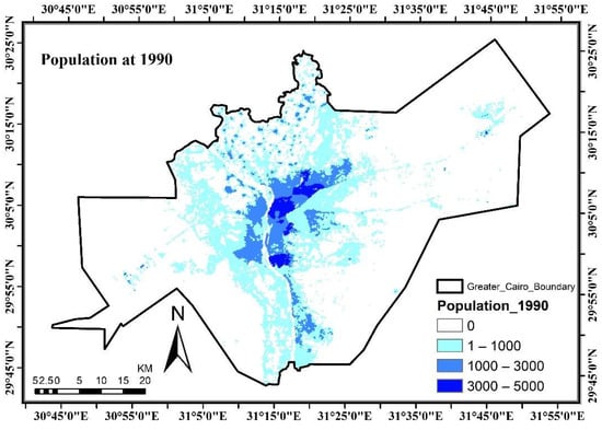
Figure 2.
Distribution of population in GC.
3.4. GIS Interpolation Method
Interpolation is a method that uses observed values or sample sites to calculate values at other unknown places. A wider range of geographic point data, including PGA, elevation, rainfall, chemical concentrations, and so on, may be projected [73]. In this study, six common interpolation approaches are evaluated and compared to demonstrate the best spatial interpolation performance for PGA data and which one of them have the best ability to generate seismic hazard maps caused by a specific earthquake.
This study examined six GIS interpolation methods (IDW, Kriging, Natural, Spline, TopoToR, Trend). IDW (Inverse Distance Weighted) can interpolate cell values [22], using the average closeness of sample data points to each processing cell. Each point’s average weight grows with its distance from the cell’s center. Kriging is an effective geo-statistical approach for estimating a point distribution’s surface. Even more than with other interpolation approaches, it is vital to investigate the spatial behavior of the phenomena represented by the z-values before generating the final surface. Using Natural Neighbor, you may discover the closest group of input data to a data instance and apply weights based on relative regions to interpolate values. It is sometimes called “Sibson interpolation” or “area-stealing.” The Spline approach interpolates data using a mathematical equation that reduces surface curvature, resulting in a smooth, flowing surface. Topo to Raster uses an interpolation method aimed at generating a surface that more closely matches an existing drainage surface while keeping ridgelines and stream systems from the input contour data. Hutchinson and colleagues created ANUDEM at the Australian National University. Trend is a polynomial interpolation method used worldwide to match input values to a smooth surface (a polynomial). The trend surface evolves gradually and catches large-scale data structures [74].
3.5. Machine Learning Methods and Evaluation Metrics
Using appropriate ML algorithms, the goal with ML is to make this operation as automated as feasible. In this study, we create many regression algorithms aiming at reaching the best suitable model based on the obtained performance. The following sections provide a quick explanation of how each regression algorithm in use works. To put it another way, we have created a taxonomy of the most frequent linear and nonlinear ML models used in our approach.
3.5.1. Employed Linear and Non-Linear Regression Models
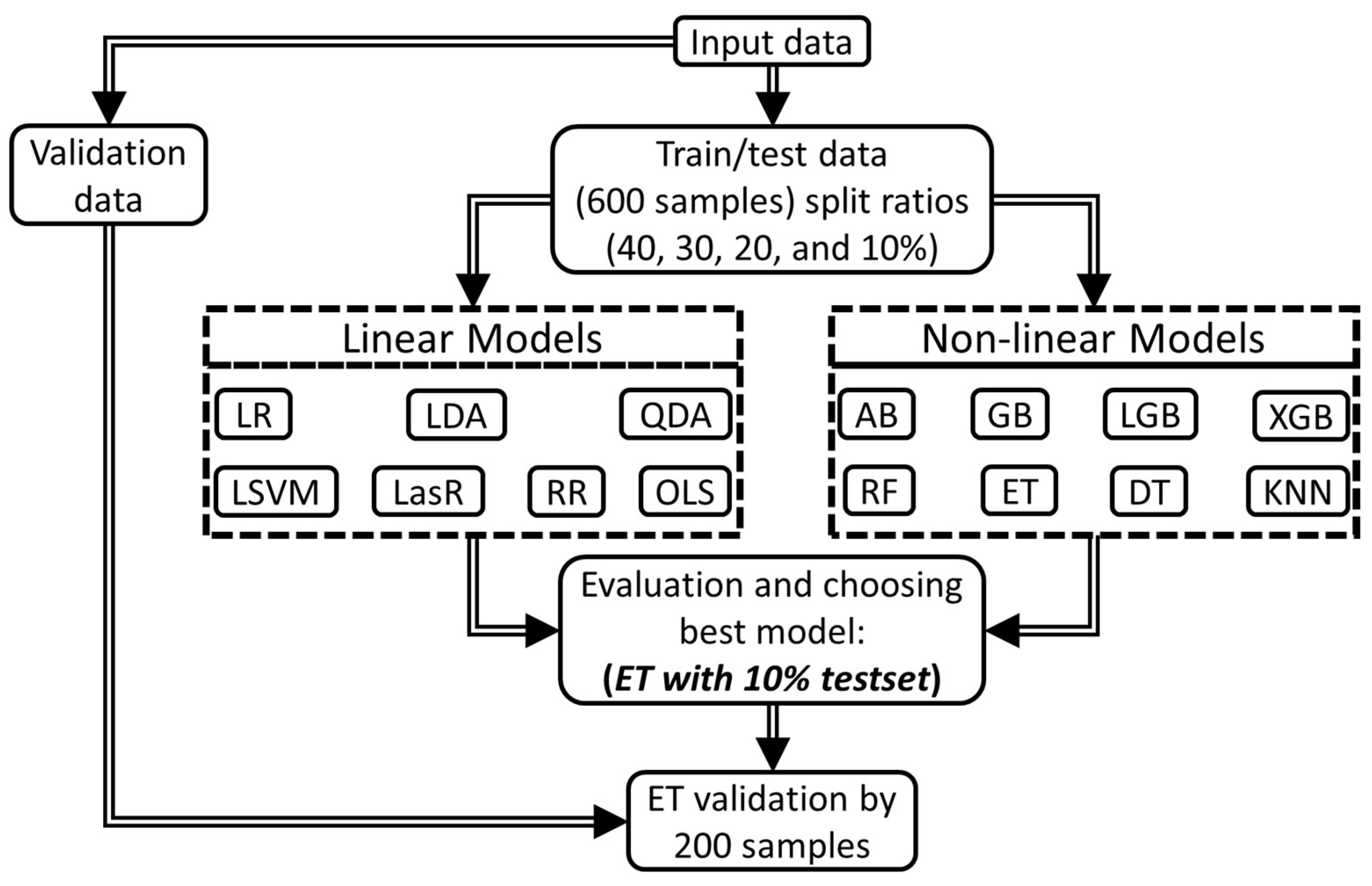
In the proposed approach, we have utilized seven linear models and eight non-linear ones as depicted in Figure 3. Figure 3 shows the proposed approach, which implements both the linear and nonlinear ML models. We have conducted extensive experimental work using the linear and non-linear ML models illustrated in Figure 3. The implemented linear models are logistic regression (LR), linear discriminant analysis (LDA), quadratic discriminant analysis (LDA), linear support vector machine (LSVM), Lasso regressor (LasR), Ridge regressor (RR), and Ordinary Least Squares regression (OLS) [30,75,76,77]. Second, the utilized non-linear models are AdaBoost (AB), Gradient Boosting (GB), Light Gradient Boosting (LGB), Extreme Gradient Boosting (XGB), random forest (RF), extra-trees (ET), decision tree (DT), and k-nearest neighbors (KNN) [75,76,78,79].

Figure 3.
ML performance evaluation and best model determination.
3.5.2. Learning and Testing Process
We have started by determining the features and targets/labels of the input dataset (800 samples). The features are represented by latitude (Lat) and longitude (Long), and the labels are the calculated PGA values. Then, the input data is handled by dividing it into three sets (training set, test set, and validation set). The training set and test set are 600 samples, while the validation set is 200 samples. First, the 600 samples are employed for training and testing the utilized models with four split ratios to 60% and 40%, 70% and 30%, 80% and 20%, and 90% and 10% for training and test, respectively. Second, the models are validated by the 200 samples by which the obtained results prove that the ET ML model achieves the best-predicted PGA values based on the utilized evaluation metrics. Accordingly, the ET model has been deployed to examine the PGA values of 48,000 location samples.
3.5.3. Performance Evaluation and Best Model Determination
We adopt both the R2, root-mean-square error (RMSE), and mean-square-error (MSE) for the models’ evaluation. Hence, it is important to discover which one is the best model. First, in statistics, the coefficient of determination, denoted R2 and pronounced “R squared”, is the proportion of the variation in the dependent variable that is predictable from the independent variable(s). This scoring value can be computed by:
where RSS is the sum of squares of residuals and TSS is the total sum of squares, which can be given by:
where is the number of observations, is the ith value to be predicted, is the predicted value, and is the mean value of the sample.
Second, the RMSE/MSE is the most commonly utilized loss function measure in the assessment process. The MSE can be given by:
where denotes the set of true values, is the Euclidean norm, and represents the predicted values set which can be given by:
where denotes the parameters that generally includes the sets of weights and bias values represented by W and b, respectively. In addition, the probability density function of the predicted values can be given by:
where is the test set used for the prediction process.
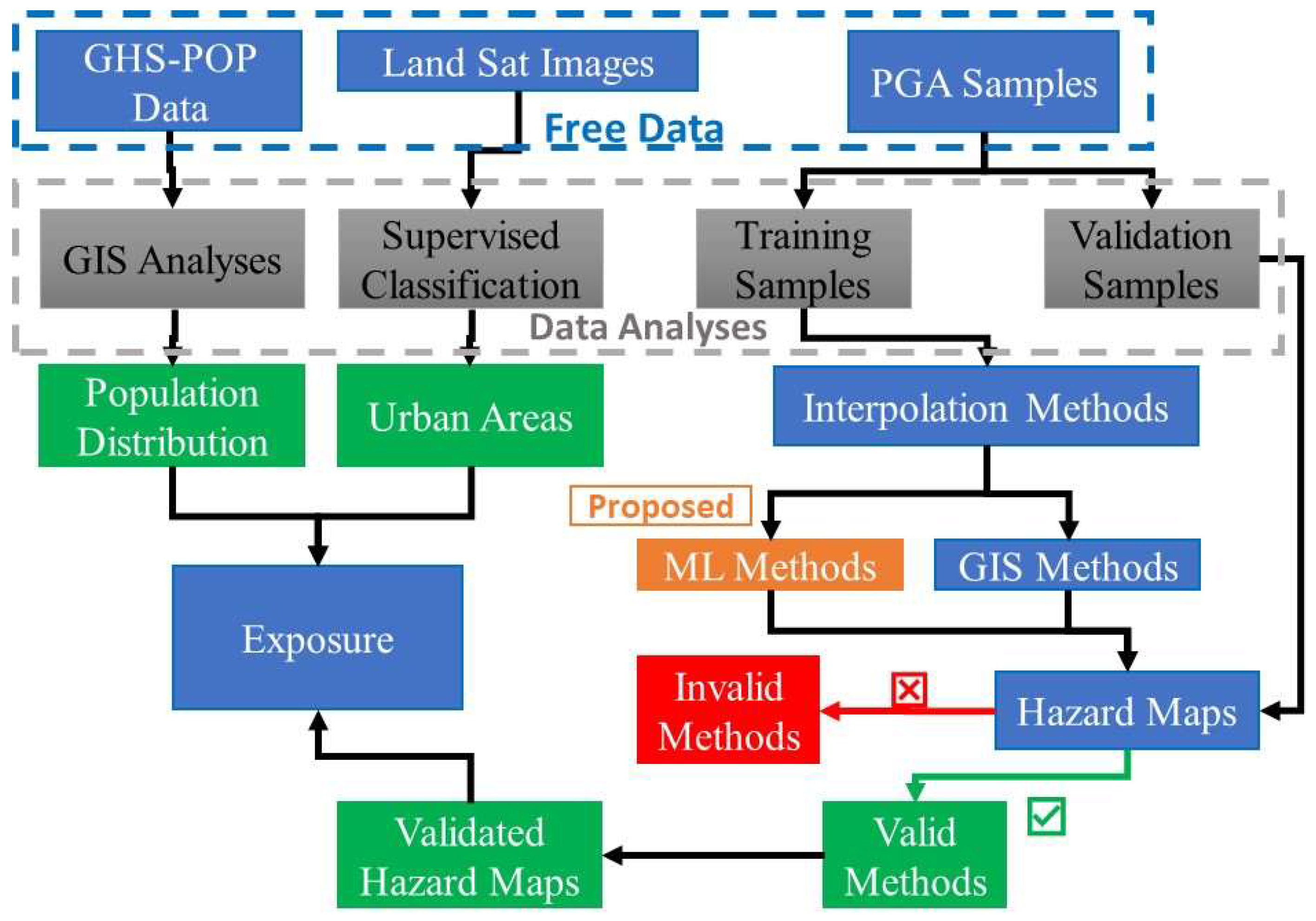
A flow chart summarizes the steps that are implemented in the current work to achieve the author’s goals is presented in Figure 4.
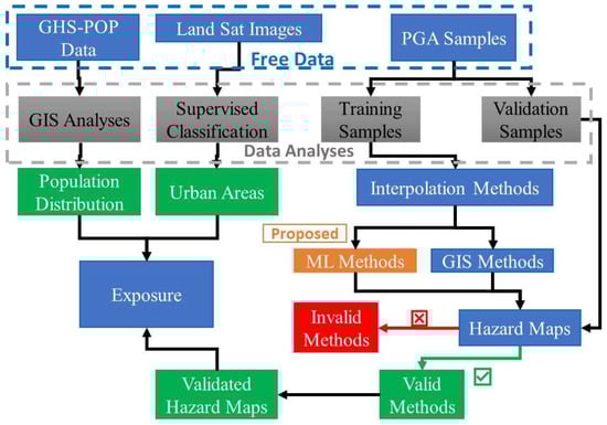
Figure 4.
The methodolgy process.
4. Results
This section will present the results of the study in five sections; each will exhibit the distinct findings depending on the sort of analysis used. The findings of the approach for identifying historical urban areas in certain years will be presented in the first section. The second part will depict the geographical distribution of the population in the study region of GC in prior years. The third section will examine and contrast between the various methods of predicting PGA distribution map. The fourth section will examine the overlap between the findings of the previous section and the results of part three in order to identify urban areas that are prone to earthquake hazard. The last section will examine sections two and three in order to determine how the population is being exposed to seismic hazards.
4.1. Identifying Historical Urban Area
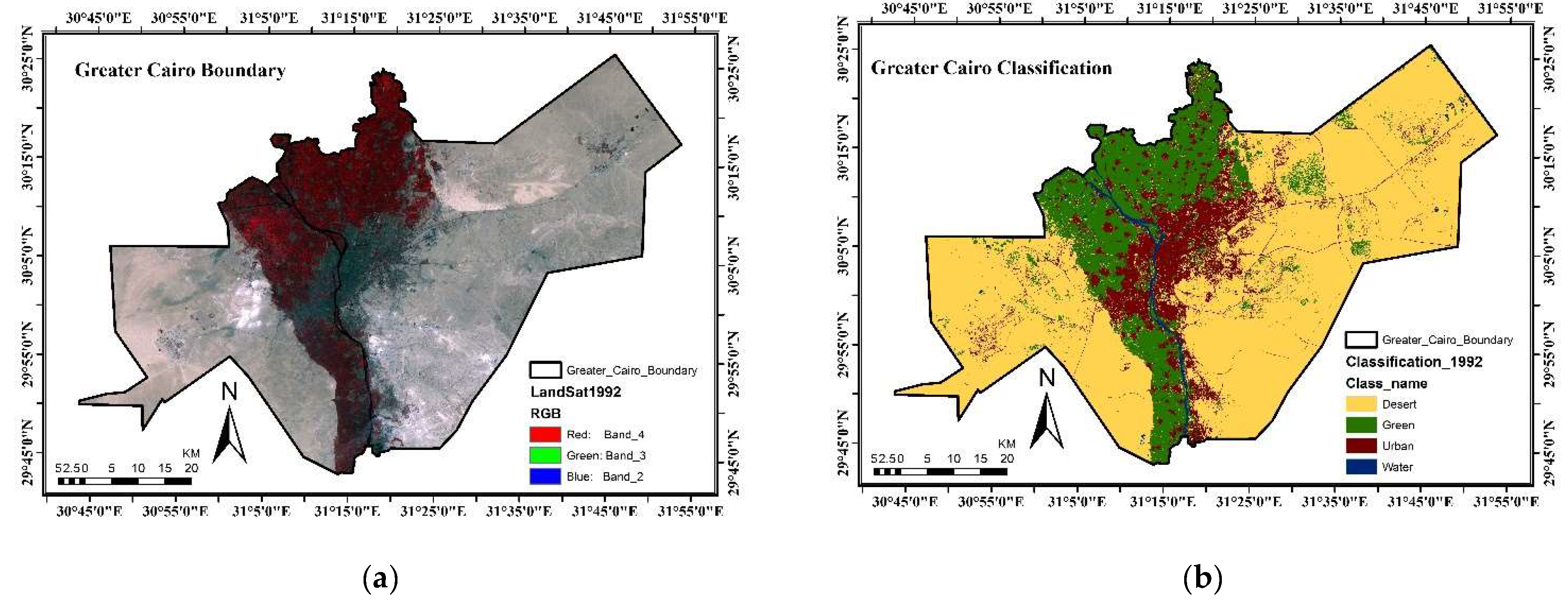
Landsat satellite images give a useful method of strewing the historical urban area, and this section will demonstrate the results of a Landsat analysis to extract the land uses in 1992. Figure 5a depicts the outcome of the first stage, which began with integrating bands for the case study region in 1992 in natural colors without the presence of an atmosphere. Figure 5b depicts the same image after being subjected to supervised classification using GIS.

Figure 5.
(a) Landsat image with natural colors; (b) Landsat Classification for GC.
The land use in GC was separated into four categories, which were as follows: desert, green, urban, and water. The desert was the most common and the water was the least type of land use in GC. The information presented in Table 2 indicates that in 1992, the deserts, green spaces, urban areas, and water areas accounted for 66.63 percent, 19.54 percent, 12.62 percent, and 1.21 percent of the region’s total land area, respectively, according to the statistics supplied. For the purposes of estimating the exposure area that is susceptible to seismic hazard, this article concentrated on urban areas; the total area of the urban class in this study was 55,085 Ha.
Table 2.
Results of Landsat classification.
A classification accuracy assessment is a critical step in order to verify the outcomes of applying supervised classification to categories the Landsat satellite images. As illustrated in Figure 6, the accuracy test for the 1992 land use map employed a total of 500 random test sites dispersed among the categorized classes in order to evaluate the classification accuracy. The Kappa coefficients were calculated based on the error matrices that were created. According to Table 3, the accuracy of class categorization varied from 0.95 for desert, 0.97 for Green and 0.79 for urban to 1 for water bodies, for a total accuracy of 93 percent, with a Kappa value of 0.87, which shows that classification accuracy is practically totally dependable [80].
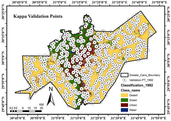
Figure 6.
Distribution of Kappa validation points.
Table 3.
Results of Kappa validation.
4.2. Identifying Seismic Hazard Map with Different Methods
In order to identify SHPs, this section of the results will compare the six GIS-based interpolation techniques indicated in Section 3.4 (IDW, Kriging, Natural, Spline, TopoToR, and Trend), as well as the proposed (ML) method, which was discussed in Section 3.5. The PGA data were recorded on 800 points (mentioned in Section 3.1) in different random locations throughout the study area. This number of points was divided into two categories: the first category contained around 600 random PGA points that were used to initiate the SHPs based on each of the seven interpolation methods. In addition, the second category contained around 200 random points that contained real PGA values that were used to extract the PGA values from the initiated SHPs, as shown in Figure 7. After that, we made a comparison between the real PGA values and the extracted PGA values from all previous SHPs.
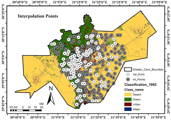
Figure 7.
Dividing PGA values to validate all interpolation methods.
Table 4 shows the obtained accuracy and error comparison of the predicted PGA values using the best-proposed ML model (ET) among the other classical models (IDW, Kriging, Natural, Spline, TopoToR, and Trend). It is noteworthy that the proposed ML model outperforms the other techniques from the highest accuracy point of view (0.96) and the minimum error (residual) one (8.54). While the techniques of Kriging and TopoToR methods with accuracy (0.95) and minimum error (9.06 and 9.45).
Table 4.
Comparison between accuracy of all interpolation methods.
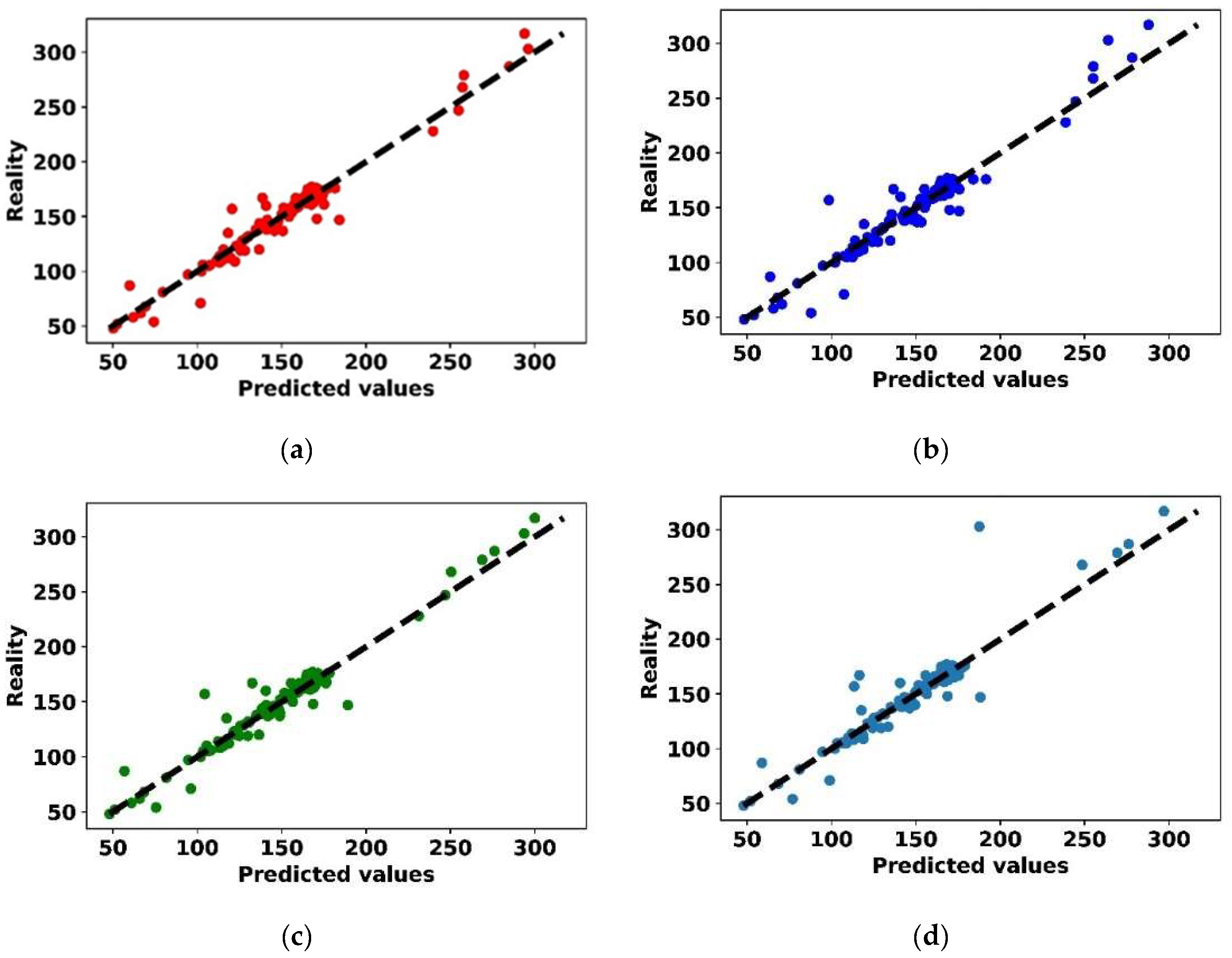
For valuable visual presentation of the predicted PGA values, we have employed both the MSE and R2 values and comparing the true values of PGA represented by the linear curve as shown in Figure 8a, and compared it with the predicted values using the best ML model. In other words, we have achieved the best-predicted values with minimal residual ones as compared to the other six classical methodologies shown in Figure 8b–g. More concretely, the predicted PGA values using the proposed ET ML model achieves the minimum fluctuations below and above the true values.
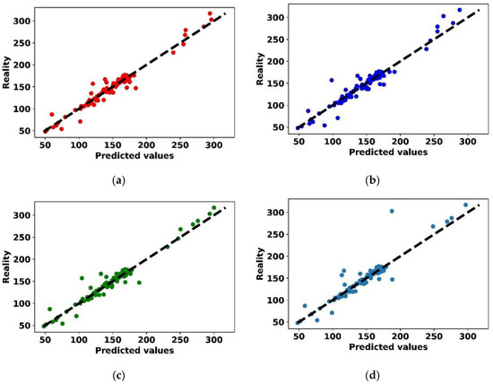
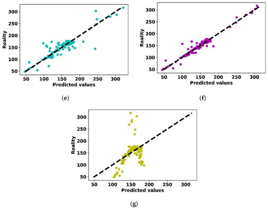
Figure 8.
Comparison between the predicted PGA values using ML along with the utilized classical interpolation methods and the calculated ones. (a) Using the proposed ML model, (b) using IDW method, (c) using Kriging, (d) using Natural method, (e) using Spline method, (f) using TopoToR method, and (g) using Trend method.
4.3. Urban Reas Exposure to Seismic Hazard
This section will describe the findings and contributions made, as well as comparing the outcomes of interpolation between the machine learning approach and those obtained via the use of GIS. In accordance with the values of the PGA, the results of interpolation for all techniques were categorized, as shown in Table 5. Table 5 shows the current PGA based intensity scale. Earthquake intensity scales describe the severity of an earthquake’s effects on the Earth’s surface, humans, and buildings at different locations in the area of the epicenter. The degree of shaking due to an earthquake event can be estimated either quantitatively in terms of the peak ground parameters or qualitatively using the felt intensity. The felt-intensity values are determined based on the observed structural damage and/or the response of humans to the ground shaking. These felt intensities are useful as an input in rapid loss modeling. The intensity scale was extended to eight levels (0 to 7) due to the widespread pattern of high ground accelerations (400 Gal and greater). At lower levels of the scale (0 to 3), the intensity is generally assessed in terms of how the shaking is felt by people. Higher levels of the scale (4 to 7) are based on observed structural damage surveyed by professionals.
Table 5.
Classification of PGA values (USGS 2003).
The classes belong to the category of perceived shaking.
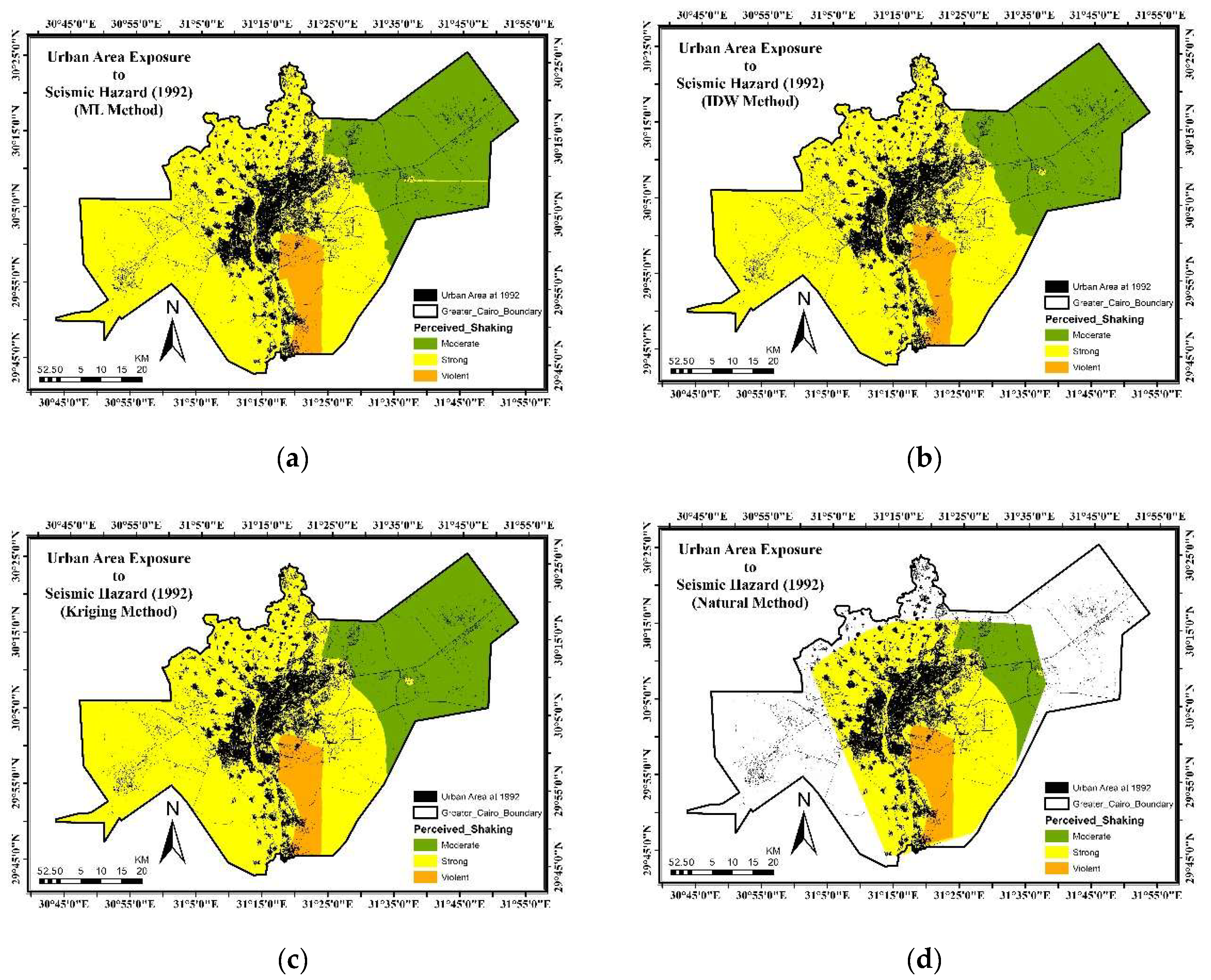
This findings section illustrates the overlap between urban areas in 1992 and several seismic hazard maps for the 12 October 1992 earthquake, in order to study the influence of selecting an interpolation method on the creation of the seismic hazard map. This stage attempts to analyze the distribution and exposure of urban areas to the perceived shaking classes across various interpolation techniques in order to determine which approach is the most effective. In Figure 9a–g, you can see an example of this.


Figure 9.
Urban area exposure and the predicted PGA values generated by different interpolation methods. (a) Using the proposed ML model, (b) using IDW method, (c) using Kriging, (d) using Natural method, (e) using Spline method, (f) using TopoToR method, and (g) using Trend method.
The values in Table 6 represent urban areas measured in hectares for each of the four classes. Statistics shows that approximately 98.15 percent of the total urban areas in GC are located in a strong perceived shaking class. This area created by the Trend method, which has the highest percentage over the other methods, while the moderate percentage was 94.47 percent, which was generated by Natural method and the lowest percentage of urban areas was approximately 87.43 percent in the same perceived shaking class, which it was generated by the Spline method. For example, as shown in Table 6, several interpolation techniques estimated different values for the distribution of urban areas, indicating to some degree that the interpolation methods are mainly showing values in three classes of perceived shaking: moderate, strong, and violent. As a result, the focus of this section will be on the classes that study it.
Table 6.
Results of urban areas exposure based on type of interpolation methods.
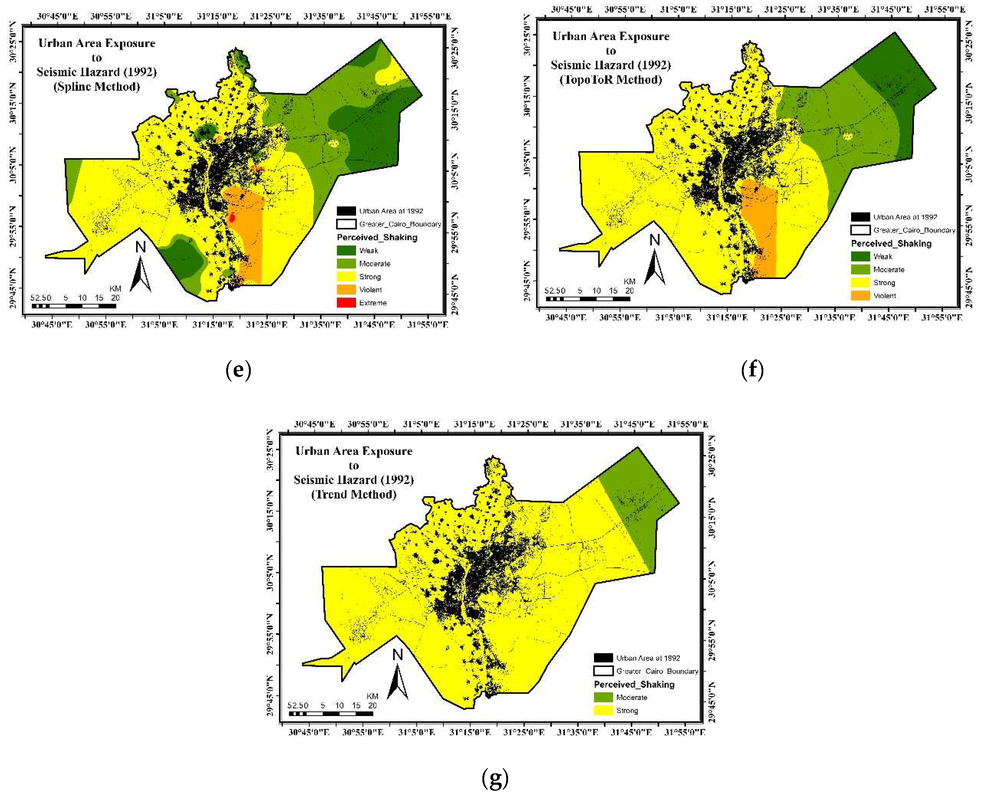
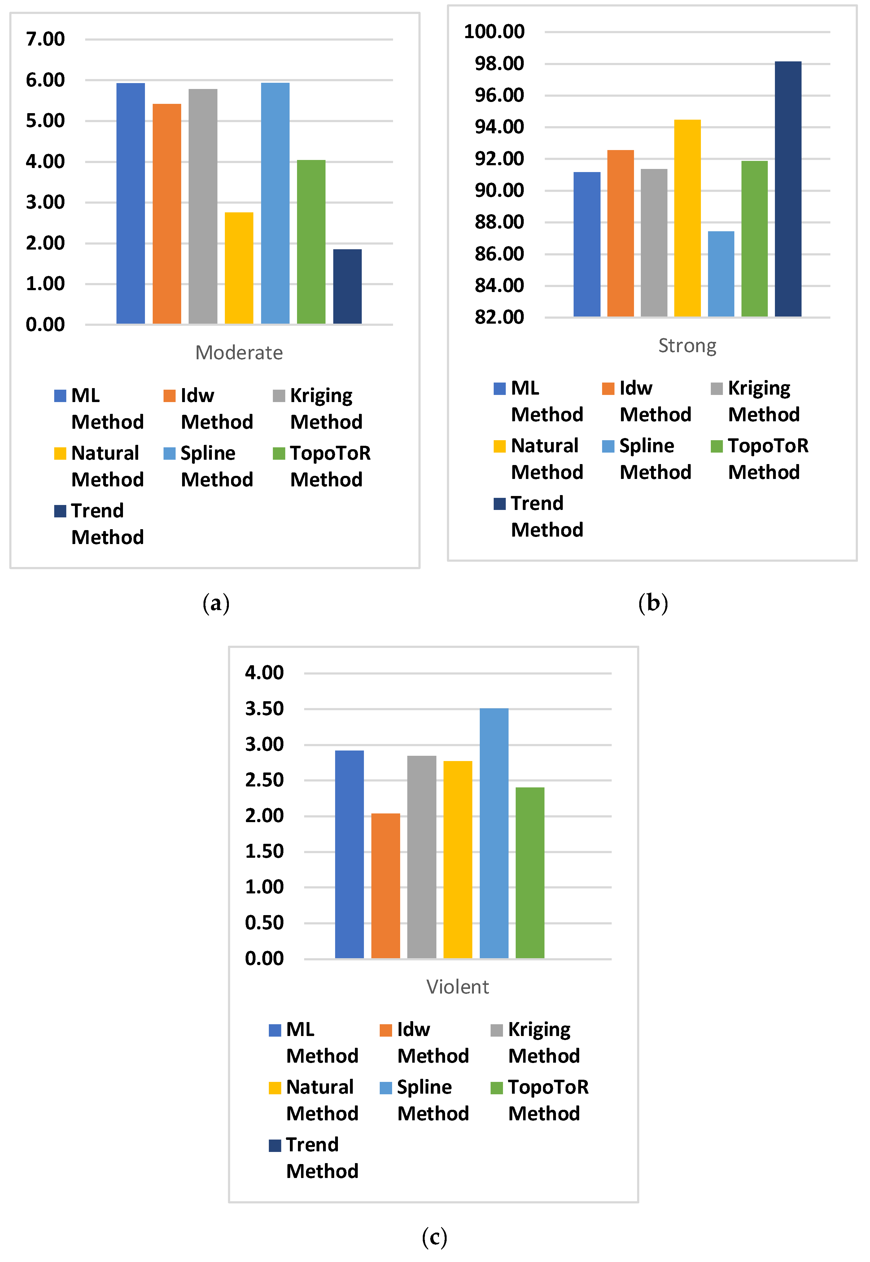
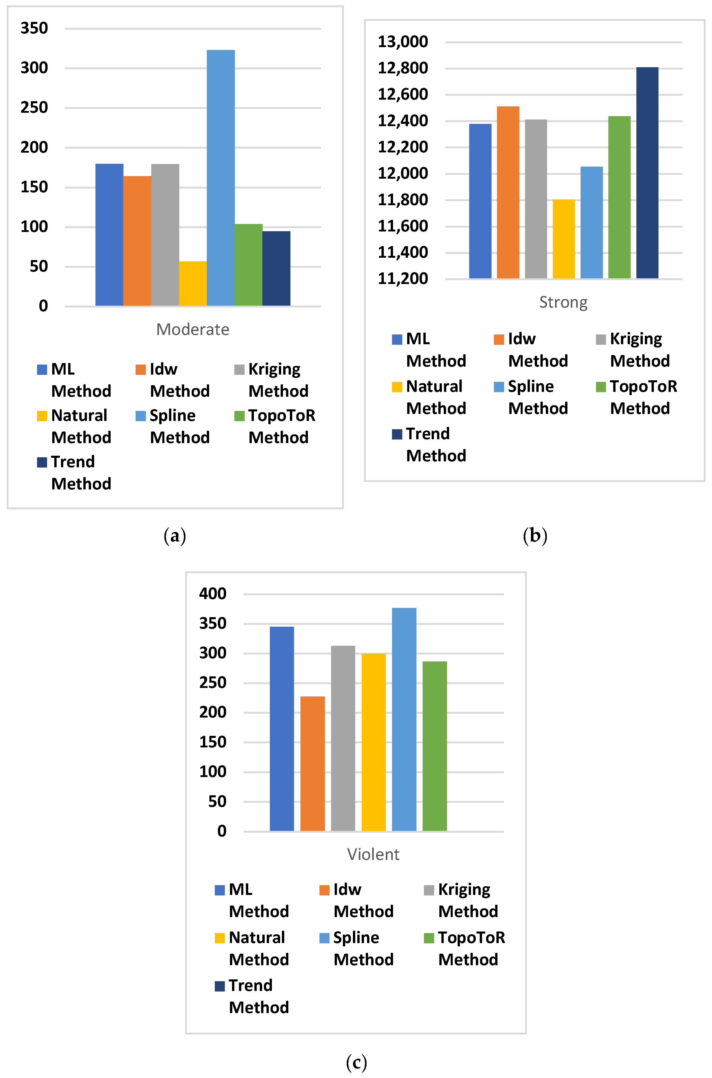
As can be seen in Figure 10a, the ML, Kriging, and Spline methods generate similar values (approximately 5.7–5.9) for urban areas that are exposed to moderate shaking. However, the other comparison in Figure 10b shows that the ML and Kriging methods also generate similar values (approximately 91.9–92.2) for urban areas exposed to moderate shaking. According to the analysis, Figure 10c, the most significant relationship can be found between the ML and Kriging methods. Following the representation of all panels of Figure 10, it can be concluded that Kriging is the closest GIS approach to the ML, and that both of them have the greatest capacity to spread the exposure of urban areas via the classes of the perceived shaking.
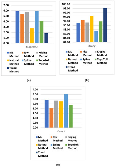
Figure 10.
Result analyses for urban area exposure using all interpolation methods. (a) Urban area analyses (moderate exposure). (b) Urban area analyses (strong exposure). (c) Urban area analyses (violent exposure).
According to Figure 10 and Table 6, one of the most significant findings was that the three methods recorded greater values for urban areas than the other methods. The first was the Natural methods in moderate and strong classes, the second was the Spline methods in strong and violent classes, and the third was the Trend method in moderate and strong classes. The last was the Trend method in strong and violent classes, and it did not record any values for urban areas in the violent class. Based on the results of the previous sections, this article can recommend the ML and Kriging methods for interpolating the predicting the earthquake shaking level as a first step in identifying the exposed urban areas in the GC. The Natural, Spline, and Trend methods are excluded from the predicting the shaking levels maps in this study.
4.4. Population Exposure to Seismic Hazard
This section examines the GHS-POP data, which provides a raster map of the world’s population. We clipped the raster population map for the GC and overlapped it with the PGA maps of 12 October 1992, which were generated by different interpolation methods. Comparing the results of that overlap gave a good indication of how to analyze the differences between different methods. According to the data in Table 7, the overall population of the GC was 12.9 million people per capita. To assess and compare the impact of interpolation techniques on population exposure for seismic hazard maps, all population spatial distributions are based on perceived shaking classes for each method, which were calculated for each method independently. The majority of the population was concentrated in the “strong class”, which accounted for 93–99 percent of the total population, while the average was concentrated in the “Violent class”> for 2–3% and the minority of the population was concentrated in “Moderate class” for 1–3%.
Table 7.
Results of population exposure based on type of interpolation methods.
In Figure 11, the relationships between the impacts of all methods on population distribution can be seen since the vast majority of the population falls into a strong class of perceived shaking. This section will be taken into consideration when you shake it. As indicated in Figure 11b, the closest values were recorded by the ML and Kriging methods, followed by TopoToR, which all recorded the same percentage (96 percent), while the furthest values were recorded by the Natural and Trend methods (97 percent and 99 percent, respectively).

Figure 11.
Result of the analyses of population exposure using different interpolation methods. (a) Population analyses (moderate exposure). (b) Population analyses (strong exposure). (c) Population analyses (violent exposure).
5. Discussion
Comparing the findings of the current article with the others obtained the literature review, the authors believe that the findings of this article may be seen as both useful and novel. The main findings of the current article can be summed up in four points as follows: The first is due to the large damage associated with the 12 October 1992 earthquake. It is considered as the most significant earthquake affecting northern Egypt. Several tries have been carried out to simulate the ground shaking caused by this event at different localities by Fayoum [81], Qalubyia [82], and Saqqara [83]. Abdel Aal et al. (2008) estimated the ground motion of this earthquake considering the local site conditions at some location located in Al-Fayoum city [81]. Amin (2015) estimated the ground motion of this event at Saqqara pyramid which is located 15 km from the epicenter of Dahshour earthquake [83]. The current study is the first one using an earthquake scenario-based approach to produce regional PGA map of the 12 October 1992 earthquake for the GC considering the local site conditions using the available geotechnical data and geophysical measurements. The geotechnical data are converted to the Vs30 using worldwide equations. The calculated Vs30 are classified according to the USGS standard. The obtained results reflect the great impact of the local site conditions on the ground motion caused by this earthquake, as mentioned by [81,83].
Second, the literature review [22,84,85,86,87] for the various articles revealed that the majority of them only compare three or four interpolation methods, whereas this article compared the default six interpolation methods that are provided by ArcGIS. This comparison is very important because it allowed the authors to make recommendations regarding the proper method that can be used to predict the PGA values and create SHMs with the highest degree of accuracy.
Third, the results of the based ML interpolation method are compared with the earlier once based on the GIS, as well as the impacts of interpolation methods on the exposure (population) located in different seismic hazard zones in the study area. It is more detailed than the analyses performed in the articles [88,89,90], which compare only one or two GIS interpolation methods and do not represent the impact of using different interpolation methods on the exposure in the metropolitan areas.
The last, ML has proved beneficial for both classification and regression problems of PGA, peak particle velocity (PPV), seismic hazard assessment, and urbanization studies [29,30,91,92,93]. Using ML learning in these studies reach 99% of detecting targets accuracy in some cases such as PPV. In [91], the proposed ML mechanism was used to determine rockfall probability relying on multiple rockfall conditioning metrics. That approach achieved accuracy of 93% and 95%. In [92], a ML learning model based on XGB attained 95% and 93% of prediction accuracy for the sustainable rural drinking water supply. For urban flood risk assessment, ML was utilized with a successful estimation accuracy of 89.2% [93]. In the current study, we have employed several linear and non-linear ML models, in which the ET model achieved the best PGA estimation accuracy with 96% among the linear and non-linear ML models. Besides, the employed ML approach outperformed the six classical GIS methods as shown in Figure 8. It is worth mentioning that the ET model is a non-linear technique which can meet the non-homogeneity of the Earth structure.
To the best of our knowledge, no similar study has considered integrated approaches to tackle the considered problem. This integration included three main differences: first, it compared the most GIS interpolation methods (six); second, it created a new machine learning-based method; and last, it used all GIS methods and the ML method in initiating SHMs. This study tests the impact of metropolitan areas and population distribution on SHMs generated.
The outcomes of this investigation were compared to other earlier studies that dealt with similar themes. The many studies that have explored data interpolation can be described as follows:
- Previous studies compared only two or three methods [94,95,96], but this study compared the majority of all six GIS methods, and much of the data supported the interpolation method, which is the most accurate.
- The second class of publications applied four or five methods to different types of data, such as climatic data, soil type, and digital elevation systems [97,98].
- This paper’s findings are in line with earlier research showing that the interpolation kriging method can improve spatial prediction accuracy in different data types [95,97,99], While others show that Inverse Distance Weighted and Kriging are nearly the same [95,96]. Kriging method was the best method. The Kriging method gives superior interpolation for unmeasured quantities [100,101,102].
Most studies employ the same accuracy and error comparison strategy as this investigation. Cross-validation uses RMSE to account for stationary spots and extrema [95,97,98]. However, in this article, R2 value and MSE were used to improve the accuracy test of all interpolation methods.
6. Conclusions
Reliable SHMs play a significant role in urban planning, seismic risk assessment, and seismic risk reduction in megacities. Obtaining such maps requires detailed geotechnical investigations, which are costly and time-consuming. In this paper, the efficiency of the common six GIS-based interpolation approaches, and several linear and non-linear ML methodologies is examined in producing SHMs (i.e., PGA map) using a limited geotechnical dataset. The previously mentioned methods were applied to the available geotechnical data occurring in the GC. Additionally, the developed model relied on open-access data such as Landsat and GHS-POP to identify the exposure distribution in SHMs. The results demonstrated that the Kriging method delivered the best performance among the utilized GIS approaches with an accuracy of 95%. Moreover, the ET ML model achieved the optimum performance in predicting PGA values with an accuracy of 96%. Finally, we recommend that decision makers in developing countries such as Egypt use the proposed methodologies for accurate estimation of the SHMs, urban areas, and populations based on the location and perceived shaking.
According to the findings of this study, the proposed machine learning-based method outperformed the rest of the GIS methods in terms of accuracy, allowing it to be used to create seismic hazard maps. In the future, it is possible to include some other affecting variables, such as topography, which require more data and may require major financing, which is one of the most significant obstacles to developing the model. Moreover, the ML model needs to be improved by using updated datasets representing different regions.
Finally, the authors would like to mention that the proposed approach has been applied to the GC. The obtained geotechnical data reflects the geological setting of the study area, where the study area is composed of three geological units. These units are not intercalated with each other. The geologic setting of the study area is considered homogenous. Therefore, applying this approach to regions with heterogenous geologic settings requires more attention. Additionally, the implemented approach cannot replace the site-specific seismic hazard studies required to obtain the ground-motion parameters that are the main inputs of the design response analysis and structure response analysis of the critical facilities, mega structures and infrastructures.
Author Contributions
Conceptualization, O.H. and M.S.A.; methodology, O.H. and M.S.A.; software, O.H. and M.S.A.; formal analysis, M.E. and H.G.; investigation, M.E. and H.G.; writing—original draft preparation, O.H. and M.S.A.; writing—review and editing, M.E. and H.G.; supervision, O.H. and M.S.A.; resources, M.E. and H.G.; data curation, M.E. and H.G.; visualization, O.H. and M.S.A.; All authors have read and agreed to the published version of the manuscript.
Funding
This work was funded by the National Research Institute of Astronomy and Geophysics (NRIAG), Helwan, Cairo, Egypt. The authors, therefore, acknowledge with thanks NRIAG technical and financial support.
Institutional Review Board Statement
Not applicable.
Informed Consent Statement
Not applicable.
Data Availability Statement
The data used to support the findings of this study are included within the article.
Conflicts of Interest
The authors declare no conflict of interest.
References
- Asadi, Y.; Samany, N.N.; Ezimand, K. Seismic Vulnerability Assessment of Urban Buildings and Traffic Networks Using Fuzzy Ordered Weighted Average. J. Mt. Sci. 2019, 16, 677–688. [Google Scholar] [CrossRef]
- Gencer, E.A. Natural Disasters, Urban Vulnerability, and Risk Management: A Theoretical Overview. In The Interplay between Urban Development, Vulnerability, and Risk Management; Springer: Berlin/Heidelberg, Germany, 2013; pp. 7–43. [Google Scholar] [CrossRef]
- Words into Action Guidelines: National Disaster Risk Assessment Hazard Specific Risk Assessment. Available online: https://www.undrr.org/publication/words-action-guidelines-national-disaster-risk-assessment (accessed on 2 April 2022).
- Frankel, A. Mapping Seismic Hazard in the Central and Eastern United States. Seismol. Res. Lett. 1995, 66, 8–21. [Google Scholar] [CrossRef]
- Moustafa, S.S.R.; Abdalzaher, M.S.; Naeem, M.; Fouda, M.M. Seismic Hazard and Site Suitability Evaluation Based on Multi-Criteria Decision Analysis. IEEE Access 2022, 10, 69511–69530. [Google Scholar] [CrossRef]
- Kim, H.S.; Sun, C.G.; Kim, M.; Cho, H.I.; Lee, M.G. GIS-Based Optimum Geospatial Characterization for Seismic Site Effect Assessment in an Inland Urban Area, South Korea. Appl. Sci. 2020, 10, 7443. [Google Scholar] [CrossRef]
- Duzgun, H.S.B.; Yucemen, M.S.; Kalaycioglu, H.S.; Celik, K.; Kemec, S.; Ertugay, K.; Deniz, A. An Integrated Earthquake Vulnerability Assessment Framework for Urban Areas. Nat. Hazards 2011, 59, 917–947. [Google Scholar] [CrossRef]
- Bostenaru Dan, M.; Armas, I.; Goretti, A. Earthquake Hazard Impact and Urban Planning; Springer Science & Business Media: Berlin/Heidelberg, Germany, 2014; pp. 1–313. [Google Scholar] [CrossRef]
- Hamdy, O.; Zhao, S.; El-atty, H.A.; Ragab, A.; Salem, M. Urban Areas Management in Developing Countries: Analysis the Urban Areas Crossed with Risk of Storm Water Drains, Aswan-Egypt. Int. J. Urban Civ. Eng. 2020, 14, 96–102. [Google Scholar]
- Ghamry, E.; Mohamed, E.K.; Abdalzaher, M.S.; Elwekeil, M.; Marchetti, D.; de Santis, A.; Hegy, M.; Yoshikawa, A.; Fathy, A. Integrating Pre-Earthquake Signatures from Different Precursor Tools. IEEE Access 2021, 9, 33268–33283. [Google Scholar] [CrossRef]
- Rikimaru, A.; Roy, P.S.; Miyatake, S. Tropical Forest Cover Density Mapping. Trop. Ecol. 2002, 43, 39–47. [Google Scholar]
- Noby, M.; Michitaka, U.; Hamdy, O. Urban Risk Assessments: Framework for Identifying Land-Uses Exposure of Coastal Cities to Sea Level Rise, a Case Study of Alexandria. SVU-Int. J. Eng. Sci. Appl. 2022, 3, 78–90. [Google Scholar] [CrossRef]
- Ramadhan Kete, S.C.; Suprihatin; Tarigan, S.D.; Effendi, H. Land Use Classification Based on Object and Pixel Using Landsat 8 OLI in Kendari City, Southeast Sulawesi Province, Indonesia. IOP Conf. Ser. Earth Environ. Sci. 2019, 284, 012019. [Google Scholar] [CrossRef]
- Schneider, A. Monitoring Land Cover Change in Urban and Peri-Urban Areas Using Dense Time Stacks of Landsat Satellite Data and a Data Mining Approach. Remote Sens. Environ. 2012, 124, 689–704. [Google Scholar] [CrossRef]
- USGS GloVis-USGS. Available online: https://earthexplorer.usgs.gov/ (accessed on 20 March 2022).
- Hamdy, O.; Zhao, S.; Salheen, M.A.; Eid, Y.Y. Identifying the Risk Areas and Urban Growth by ArcGIS-Tools. Geosciences 2016, 6, 47. [Google Scholar] [CrossRef]
- Freire, S.; Macmanus, K.; Pesaresi, M.; Doxsey-Whitfield, E. Development of New Open and Free Multi-Temporal Global Population Grids at 250 m Resolution Validation of Remote Sensing Derived Emergency Mapping Maps View Project Megacities View Project. 2016. Available online: https://publications.jrc.ec.europa.eu/repository/handle/JRC100523 (accessed on 2 April 2022).
- Schiavina, M.; Freire, S.; MacManus, K. Global Human Settlement-GHS-POP-European Commission. Available online: https://ghsl.jrc.ec.europa.eu/ghs_pop2019.php (accessed on 20 March 2022).
- Florczyk, A.J.; Corbane, C.; Ehrlich, D.; Freire, S.; Kemper, T.; Maffenini, L.; Melchiorri, M.; Pesaresi, M.; Politis, P.; Schiavina, M. GHSL Data Package 2019. Luxemb. EUR 2019, 29788, 290498. [Google Scholar]
- Abdalzaher, M.S.; Elsayed, H.A. Employing Data Communication Networks for Managing Safer Evacuation during Earthquake Disaster. Simul. Model. Pract. Theory 2019, 94, 379–394. [Google Scholar] [CrossRef]
- Calka, B.; Bielecka, E. GHS-POP Accuracy Assessment: Poland and Portugal Case Study. Remote Sens. 2020, 12, 1105. [Google Scholar] [CrossRef]
- Wang, H.; Wang, Y. Analysis of Spatial Interpolation Methods. In Recent Advances in Computer Science and Information Engineering; Qian, Z., Cao, L., Su, W., Wang, T., Yang, H., Eds.; Springer: Berlin/Heidelberg, Germany, 2012; Volume 6, pp. 507–512. ISBN 978-3-642-25778-0. [Google Scholar]
- Hamdy, O.; Zhao, S.; Salheen, M.; Eid, Y. Using Arc GIS to Analyse Urban Growth towards Torrent Risk Areas (Aswan City as a Case Study). IOP Conf. Ser. Earth Environ. Sci. 2014, 20, 12009. [Google Scholar] [CrossRef]
- McCoy, J.T.; Auret, L. Machine Learning Applications in Minerals Processing: A Review. Miner. Eng. 2019, 132, 95–109. [Google Scholar] [CrossRef]
- Mohammed, M.; Khan, M.B.; Bashier, E.B.M. Machine Learning: Algorithms and Applications; CRC Press: Boca Raton, FL, USA, 2016; ISBN 1498705391. [Google Scholar]
- Abdalzaher, M.S.; Elwekeil, M.; Wang, T.; Zhang, S. A Deep Autoencoder Trust Model for Mitigating Jamming Attack in IoT Assisted by Cognitive Radio. IEEE Syst. J. 2021, 1–11. [Google Scholar] [CrossRef]
- Pradhan, B. A Comparative Study on the Predictive Ability of the Decision Tree, Support Vector Machine and Neuro-Fuzzy Models in Landslide Susceptibility Mapping Using GIS. Comput. Geosci. 2013, 51, 350–365. [Google Scholar] [CrossRef]
- Abdalzaher, M.S.; Soliman, M.S.; El-Hady, S.M.; Benslimane, A.; Elwekeil, M. A Deep Learning Model for Earthquake Parameters Observation in IoT System-Based Earthquake Early Warning. IEEE Internet Things J. 2021, 9, 8412–8424. [Google Scholar] [CrossRef]
- Moustafa, S.S.R.; Abdalzaher, M.S.; Yassien, M.H.; Wang, T.; Elwekeil, M.; Hafiez, H.E.A. Development of an Optimized Regression Model to Predict Blast-Driven Ground Vibrations. IEEE Access 2021, 9, 31826–31841. [Google Scholar] [CrossRef]
- Abdalzaher, M.S.; Moustafa, S.S.R.; Abd-Elnaby, M.; Elwekeil, M. Comparative Performance Assessments of Machine-Learning Methods for Artificial Seismic Sources Discrimination. IEEE Access 2021, 9, 65524–65535. [Google Scholar] [CrossRef]
- Moustafa, S.S.R.; Abdalzaher, M.S.; Khan, F.; Metwaly, M.; Elawadi, E.A.; Al-Arifi, N.S. A Quantitative Site-Specific Classification Approach Based on Affinity Propagation Clustering. IEEE Access 2021, 9, 155297–155313. [Google Scholar] [CrossRef]
- Maamoun, M.; Megahed, A.; Allam, A. Seismicity of Egypt. Bull. HIAG 1984, 4, 109–160. [Google Scholar]
- Ambraseys, N.N.; Melville, C.P.; Adams, R.D. The Seismicity of Egypt, Arabia and the Red Sea: A Historical Review; Cambridge University Press: Cambridge, UK, 1994. [Google Scholar]
- Sawires, R.; Peláez, J.A.; Fat-Helbary, R.E.; Ibrahim, H.A. An Earthquake Catalogue (2200 B.C. to 2013) for Seismotectonic and Seismic Hazard Assessment Studies in Egypt. In Earthquakes and Their Impact on Society; Springer: Berlin/Heidelberg, Germany, 2016; pp. 97–136. [Google Scholar] [CrossRef]
- El-Sayed, A.; Arvidsson, R.; Kulhánek, O. The 1992 Cairo Earthquake: A Case Study of a Small Destructive Event. J. Seismol. 1998, 2, 293–302. [Google Scholar] [CrossRef]
- Badawi, H.S.; Mourad, S.A. Observations from the 12 October 1992 Dahshour Earthquake in Egypt. Nat. Hazards 1994, 10, 261–274. [Google Scholar] [CrossRef]
- Badawy, A.; Korrat, I.; El-Hadidy, M.; Gaber, H. Probabilistic Earthquake Hazard Analysis for Cairo, Egypt. J. Seismol. 2016, 20, 449–461. [Google Scholar] [CrossRef]
- Mohamed, A.M.S.; Mohamed, G.E.A.; Omar, K.; Nadia, A.A. Present Stage of Recent Crustal Movements and Seismicity within Greater Cairo Area, Egypt. J. Seismol. 2014, 18, 23–35. [Google Scholar] [CrossRef]
- Abdalzaher, M.S.; El-Hadidy, M.; Gaber, H.; Badawy, A. Seismic Hazard Maps of Egypt Based on Spatially Smoothed Seismicity Model and Recent Seismotectonic Models. J. Afr. Earth Sci. 2020, 170, 103894. [Google Scholar] [CrossRef]
- Salem, M.; Tsurusaki, N.; Divigalpitiya, P.; Osman, T.; Hamdy, O.; Kenawy, E.; Barbini, A.; Malacarne, G.; Romagnoli, K.; Massari, G.A. Assessing Progress towards Sustainable Development in the Urban Periphery: A Case of Greater Cairo, Egypt. Int. J. Sustain. Dev. Plan. 2020, 15, 971–982. [Google Scholar] [CrossRef]
- Hamdy, O. Using Remote Sensing Techniques to Assess the Changes in the Rate of Urban Green Spaces in Egypt: A Case Study of Greater Cairo. Int. Des. J. 2022, 12, 53–64. [Google Scholar] [CrossRef]
- Dorra, E.M. Greater Cairo Earthquake Loss Assessment and Its Implications on the Egyptian Economy. Ph.D. Thesis, Imperial College London, London, UK, 2011. [Google Scholar]
- Dorra, E.M.; Stafford, P.J.; Elghazouli, A.Y. Seismic Vulnerability of Lifelines in Greater Cairo. In Proceedings of the 15th World Conference on Earthquake Engineering, Lisbon, Portugal, 24–28 September 2012. [Google Scholar]
- Osman, T.; Divigalpitiya, P.; Osman, M.M.; Kenawy, E.; Salem, M.; Hamdy, O. Quantifying the Relationship between the Built Environment Attributes and Urban Sustainability Potentials for Housing Areas. Buildings 2016, 6, 39. [Google Scholar] [CrossRef]
- General Organization for Physical Planning (GOPP). Greater Cairo Urban Development Strategy: Part I: Future Vision and Strategic Directions; Ministry of Housing, Utilities, and Urban Communities (MHUC): Cairo, Egypt, 2012; pp. 1–223. [Google Scholar]
- Osman, T.; Shaw, D.; Kenawy, E. An Integrated Land Use Change Model to Simulate and Predict the Future of Greater Cairo Metropolitan Region. J. Land Use Sci. 2019, 13, 565–584. [Google Scholar] [CrossRef]
- Salem, M.; Tsurusaki, N.; Divigalpitiya, P. Remote Sensing-Based Detection of Agricultural Land Losses around Greater Cairo since the Egyptian Revolution of 2011. Land Use Policy 2020, 97, 104744. [Google Scholar] [CrossRef]
- Salem, M.; Tsurusaki, N.; Divigalpitiya, P.; Osman, T. Driving Factors of Urban Expansion in Peri-Urban Areas of Greater Cairo Region. In REAL CORP 2018–EXPANDING CITIES–DIMINISHING SPACE Are “Smart Cities” the Solution or Part of the Problem of Continuous Urbanisation around the Globe? Proceedings of the 23rd International Conference on Urban Planning, Regional Development and Information Society GeoMultimedia 2018, Vienna, Austria, 4–6 April 2018; CORP—Compentence Center of Urban and Regional Planning: Vienna, Austria, 2018. [Google Scholar]
- Douglas, J. Earthquake Ground Motion Estimation Using Strong-Motion Records: A Review of Equations for the Estimation of Peak Ground Acceleration and Response Spectral Ordinates. Earth-Sci. Rev. 2003, 61, 43–104. [Google Scholar] [CrossRef]
- Deif, A. Seismic Hazard Assessment in and around Egypt in Relation to Plate Tectonics. Ph.D. Thesis, Ain Shams University, Cairo, Egypt, 1998. [Google Scholar]
- El-Hadidy, M. Seismotectonics and Seismic Hazard Studies for Sinai Peninsula, Egypt. Master’s Thesis, Ain Shams University, Cairo, Egypt, 2008. [Google Scholar]
- Mohamed, A.E.-E.A.; El-Hadidy, M.; Deif, A.; Abou Elenean, K. Seismic Hazard Studies in Egypt. NRIAG J. Astron. Geophys. 2012, 1, 119–140. [Google Scholar] [CrossRef]
- Deif, A.; Elenean, K.A.; El Hadidy, M.; Tealeb, A.; Mohamed, A. Probabilistic Seismic Hazard Maps for Sinai Peninsula, Egypt. J. Geophys. Eng. 2009, 6, 288–297. [Google Scholar] [CrossRef]
- Gaber, H.; El-Hadidy, M.; Badawy, A. Up-to-Date Probabilistic Earthquake Hazard Maps for Egypt. Pure Appl. Geophys. 2018, 175, 2693–2720. [Google Scholar] [CrossRef]
- Abrahamson, N.A.; Silva, W.J.; Kamai, R. Summary of the ASK14 Ground Motion Relation for Active Crustal Regions. Earthq. Spectra 2014, 30, 1025–1055. [Google Scholar] [CrossRef]
- Ghareeb, S. Selection and Evaluation Suitable Ground Motion Prediction Equation for Seismic Hazard Assessment in Northern Egypt. Master’s Thesis, Sohag University, Sohag, Egypt, 2018. [Google Scholar]
- Elhadidy, M.; Abdalzaher, M.S.; Gaber, H. Up-to-Date PSHA along the Gulf of Aqaba-Dead Sea Transform Fault. Soil Dyn. Earthq. Eng. 2021, 148, 106835. [Google Scholar] [CrossRef]
- Said, R. The Geology of Egypt; A.A. Balkema: Rotterdam, The Netherlands, 1990; ISBN 9061918561. [Google Scholar]
- Youssef, M.I. Structural Pattern of Egypt and Its Interpretation. AAPG Bull. 1968, 52, 601–614. [Google Scholar]
- Issawi, B. Geology of the Southwestern Desert of Egypt. Ann. Geol. Surv. Egypt 1981, 11, 57–66. [Google Scholar]
- Boore, D.M. Estimating V s (30)(or NEHRP Site Classes) from Shallow Velocity Models (Depths <30 m). Bull. Seismol. Soc. Am. 2004, 94, 591–597. [Google Scholar]
- Imai, T.; Tonouchi, K. Correlation of N Value with S-Wave Velocity and Shear Modulus. In Penetration Testing, Proceedings of the 2nd European Symposium, Amsterdam, The Netherlands, 27 May 1982; Routledge: London, UK, 1982. [Google Scholar] [CrossRef]
- Toni, M. Site Response and Seismic Hazard Assessment for the Southern Part of Cairo City, Egypt. Ph.D. Thesis, Helwan University, Helwan, Egypt, 2012. [Google Scholar]
- Classifying Landsat Image Services to Make a Land Cover Map. Available online: https://www.esri.com/arcgis-blog/products/product/imagery/classifying-landsat-image-services-to-make-a-land-cover-map/ (accessed on 27 December 2021).
- Cohen, J. A Coefficient of Agreement for Nominal Scales. Educ. Psychol. Meas. 1960, 20, 37–46. [Google Scholar] [CrossRef]
- Alsonny, Z.; Ahmed, A.M.M.A.; Hamdy, O. Studying the Effect of Urban Green Spaces Location on Urban Heat Island in Cities Using Remote Sensing Techniques, 6th October City as a Case Study. Int. Des. J. 2022, 12, 243–262. [Google Scholar] [CrossRef]
- Van Vliet, J.; Bregt, A.K.; Hagen-Zanker, A. Revisiting Kappa to Account for Change in the Accuracy Assessment of Land-Use Change Models. Ecol. Model. 2011, 222, 1367–1375. [Google Scholar] [CrossRef]
- Hamdy, O.; Zhao, S. A Study on Urban Growth in Torrent Risk Areas in Aswan, Egypt. J. Archit. Plan. (Trans. AIJ) 2016, 81, 1733–1741. [Google Scholar] [CrossRef]
- Hamdy, O.; Alsonny, Z. Assessing the Impacts of Land Use Diversity on Urban Heat Island in New Cities in Egypt, Tiba City as a Case Study. Int. Des. J. 2022, 12, 93–103. [Google Scholar] [CrossRef]
- Alsonny, Z.; Hamdy, O. Procedural Framework for Assessing the Impact of New Cities Growth on Urban Heat Island, A Case Study of 6th October City. SVU-Int. J. Eng. Sci. Appl. 2022, 3, 64–78. [Google Scholar] [CrossRef]
- Accuracy Assessment for Image Classification—ArcMap|Documentation. Available online: https://desktop.arcgis.com/en/arcmap/latest/manage-data/raster-and-images/accuracy-assessment-for-image-classification.htm (accessed on 27 December 2021).
- Compute Confusion Matrix (Spatial Analyst)—ArcMap|Documentation. Available online: https://desktop.arcgis.com/en/arcmap/latest/tools/spatial-analyst-toolbox/compute-confusion-matrix.htm (accessed on 27 December 2021).
- Types of Interpolation-Advantages and Disadvantages. Available online: https://gisresources.com/types-interpolation-methods_3/ (accessed on 24 December 2021).
- Comparing Interpolation Methods—ArcMap|Documentation. Available online: https://desktop.arcgis.com/en/arcmap/latest/tools/3d-analyst-toolbox/comparing-interpolation-methods.htm (accessed on 24 December 2021).
- James, G.; Witten, D.; Hastie, T.; Tibshirani, R. An Introduction to Statistical Learning; Springer: Berlin/Heidelberg, Germany, 2013; Volume 112. [Google Scholar]
- Abdalzaher, M.S.; Seddik, K.; Muta, O. Using Repeated Game for Maximizing High Priority Data Trustworthiness in Wireless Sensor Networks. In Proceedings of the 2017 IEEE Symposium on Computers and Communications (ISCC), Heraklion, Greece, 3–6 July 2017; pp. 552–557. [Google Scholar]
- Kleinbaum, D.G.; Dietz, K.; Gail, M.; Klein, M.; Klein, M. Logistic Regression; Springer: Berlin/Heidelberg, Germany, 2002; ISBN 0387953973. [Google Scholar]
- Ahmad, M.W.; Mourshed, M.; Rezgui, Y. Trees vs Neurons: Comparison between Random Forest and ANN for High-Resolution Prediction of Building Energy Consumption. Energy Build. 2017, 147, 77–89. [Google Scholar] [CrossRef]
- Hastie, T.; Rosset, S.; Zhu, J.; Zou, H. Multi-Class Adaboost. Stat. Its Interface 2009, 2, 349–360. [Google Scholar] [CrossRef]
- Audigé, L.; Bhandari, M.; Kellam, J. How Reliable Are Reliability Studies of Fracture Classifications? A Systematic Review of Their Methodologies. Acta Orthop. Scand. 2004, 75, 184–194. [Google Scholar] [CrossRef] [PubMed]
- Abd El-Aal, A.E.-A.K. Simulating Time-Histories and Pseudo-Spectral Accelerations from the 1992 Cairo Earthquake at the Proposed El-Fayoum New City Site, Egypt. Acta Geophys. 2008, 56, 1025–1042. [Google Scholar] [CrossRef]
- Omar, K.; Attia, M.; Fergany, E.S.; Hassoup, A.; Elkhashab, H. Modeling of Strong Ground Motion during the 1992 Cairo Earthquake in the Urban Area Northern Greater of Cairo, Egypt. NRIAG J. Astron. Geophys. 2013, 2, 166–174. [Google Scholar] [CrossRef]
- Khalil, A.E. Earthquake Ground Motion Simulation during 1992 Cairo Earthquake at Saqqara Pyramid. NRIAG J. Astron. Geophys. 2015, 6, 52–59. [Google Scholar] [CrossRef]
- Moradia, S.; Fadaeib, H.; abdolalipour Adlc, A.; Ataellahid, S. Interpolation Methods in Identification Seismic Space Risk of Earthquake Case Study: 50 Km Radius of Sarpol-e Zahab City, Kermanshah Province. In Proceedings of the 2nd International Congress on Engineering, Technology and Innovation, Darmstadt, Germany, 24–26 April 2020. [Google Scholar]
- Kim, H.-S.; Sun, C.-G.; Cho, H.-I. Geospatial Big Data-Based Geostatistical Zonation of Seismic Site Effects in Seoul Metropolitan Area. ISPRS Int. J. Geo-Inf. 2017, 6, 174. [Google Scholar] [CrossRef]
- Asadi Oskouei, E.; Delsouz Khaki, B.; Kouzegaran, S.; Navidi, M.N.; Haghighatd, M.; Davatgar, N.; Lopez-Baeza, E. Mapping Climate Zones of Iran Using Hybrid Interpolation Methods. Remote Sens. 2022, 14, 2632. [Google Scholar] [CrossRef]
- Yang, R.; Xing, B. A Comparison of the Performance of Different Interpolation Methods in Replicating Rainfall Magnitudes under Different Climatic Conditions in Chongqing Province (China). Atmosphere 2021, 12, 1318. [Google Scholar] [CrossRef]
- Lee, S.; Panahi, M.; Pourghasemi, H.R.; Shahabi, H.; Alizadeh, M.; Shirzadi, A.; Khosravi, K.; Melesse, A.M.; Yekrangnia, M.; Rezaie, F. Sevucas: A Novel Gis-Based Machine Learning Software for Seismic Vulnerability Assessment. Appl. Sci. 2019, 9, 3495. [Google Scholar] [CrossRef]
- Li, C.; Men, B.; Yin, S. Spatiotemporal Variation of Groundwater Extraction Intensity Based on Geostatistics—Set Pair Analysis in Daxing District of Beijing, China. Sustainability 2022, 14, 4341. [Google Scholar] [CrossRef]
- Ghayamghamian, M.R.; Panah, A.K.; Behroo, R.; Govahi, N. Application of Interpolation Methods for Peak Ground Acceleration Estimation in Emergency Management of Metropolises. In GeoFlorida 2010: Advances in Analysis, Modeling & Design; Geotechnical Special Publication: Orlando, FL, USA, 2010; pp. 2999–3008. [Google Scholar] [CrossRef]
- Fanos, A.M.; Pradhan, B.; Alamri, A.; Lee, C.W. Machine Learning-Based and 3d Kinematic Models for Rockfall Hazard Assessment Using LiDAR Data and GIS. Remote Sens. 2020, 12, 1755. [Google Scholar] [CrossRef]
- Li, X.; Wu, X.; Sun, M.; Yang, S.; Song, W. A Novel Intelligent Leakage Monitoring-Warning System for Sustainable Rural Drinking Water Supply. Sustainability 2022, 14, 6079. [Google Scholar] [CrossRef]
- Taromideh, F.; Fazloula, R.; Choubin, B.; Emadi, A.; Berndtsson, R. Urban Flood Risk Assessment: Integration of Decision Making and Machine Learning. Sustainability 2022, 14, 4483. [Google Scholar] [CrossRef]
- AlHamaydeh, M.; Al-Shamsi, G.; Aly, N.; Ali, T. Seismic Risk Quantification and GIS-Based Seismic Risk Maps for Dubai-UAE_Dataset. Data Brief 2021, 39, 107566. [Google Scholar] [CrossRef]
- Cao, W.; Hu, J.; Yu, X. A Study on Temperature Interpolation Methods Based on GIS. In Proceedings of the 2009 17th International Conference on Geoinformatics, Fairfax, VA, USA, 12–14 August 2009; IEEE: New York, NY, USA, 2009; pp. 1–5. [Google Scholar]
- Setianto, A.; Triandini, T. Comparison of Kriging and Inverse Distance Weighted (IDW) Interpolation Methods in Lineament Extraction and Analysis. J. Appl. Geol. 2013, 5, 21–29. [Google Scholar] [CrossRef]
- Ding, Y.; Wang, Y.; Miao, Q. Research on the Spatial Interpolation Methods of Soil Moisture Based on GIS. In Proceedings of the International Conference on Information Science and Technology, Nanjing, China, 26–28 March 2011; IEEE: New York, NY, USA, 2011; pp. 709–711. [Google Scholar]
- Bhunia, G.S.; Shit, P.K.; Maiti, R. Comparison of GIS-Based Interpolation Methods for Spatial Distribution of Soil Organic Carbon (SOC). J. Saudi Soc. Agric. Sci. 2018, 17, 114–126. [Google Scholar] [CrossRef]
- Meng, Q.; Liu, Z.; Borders, B.E. Assessment of Regression Kriging for Spatial Interpolation-Comparisons of Seven GIS Interpolation Methods. Cartogr. Geogr. Inf. Sci. 2013, 40, 28–39. [Google Scholar] [CrossRef]
- Tripathi, R.; Nayak, A.K.; Shahid, M.; Raja, R.; Panda, B.B.; Mohanty, S.; Kumar, A.; Lal, B.; Gautam, P.; Sahoo, R.N. Characterizing Spatial Variability of Soil Properties in Salt Affected Coastal India Using Geostatistics and Kriging. Arab. J. Geosci. 2015, 8, 10693–10703. [Google Scholar] [CrossRef]
- Venteris, E.R.; May, C.J. Cost-Effective Mapping of Benthic Habitats in Inland Reservoirs through Split-Beam Sonar, Indicator Kriging, and Historical Geologic Data. PLoS ONE 2014, 9, e95940. [Google Scholar] [CrossRef]
- Varouchakis, E.A.; Hristopulos, D.T. Comparison of Stochastic and Deterministic Methods for Mapping Groundwater Level Spatial Variability in Sparsely Monitored Basins. Environ. Monit. Assess. 2013, 185, 1–19. [Google Scholar] [CrossRef]


Publisher’s Note: MDPI stays neutral with regard to jurisdictional claims in published maps and institutional affiliations. |
© 2022 by the authors. Licensee MDPI, Basel, Switzerland. This article is an open access article distributed under the terms and conditions of the Creative Commons Attribution (CC BY) license (https://creativecommons.org/licenses/by/4.0/).