1. Introduction
Time series forecasting problems often arise in different fields. In situations with a high uncertainty of historical data, fuzzy time series forecasting methods are more suitable. The initial data are transformed into a form of fuzzy linguistic categories and these categories are foundation for the forecasting.
Taking into account sufficiently high uncertainty of historical migration data for prospective evaluation of net migration in Latvia, three well-known fuzzy time series forecasting methods are used in this paper.
This paper’s basic purposes are:
Net migration fuzzy forecasting in Latvia using three selected methods.
The analysis of received results to determine the most suitable fuzzy forecasting method.
Practical recommendations to develop stabilization of migration flows in Latvia.
This paper’s novelty: according to the authors’ information, it is the first attempt to use fuzzy time series for migration flows forecasting.
This paper’s scientific and practical contributions are the expansion of fuzzy time series forecasting approaches to the new direction and using the received results to make practical recommendations concerning migration flow stabilization and reaching relative symmetry.
Research findings:
The whole symmetry of immigration and emigration flows is an unattainable ideal. The situation in countries with prevalent emigration flows, which is currently typical for Latvia, leads to essential outflow of trained workers and creates worse conditions for business functioning. Countries with prevalent immigration flows of untrained workers can have problems with maintenance costs. Therefore, migration flows’ symmetry is an important factor for the successful progress of any state.
This article has the following structure. In
Section 2, definitions of migration and migration flows are presented, and the state of migration flows in Latvia is described.
Section 3 provides a review of the relevant literature on fuzzy time series forecasting methods.
Section 4 discusses the conceptual foundations of fuzzy time series and common approaches to their prediction.
Section 5 presents net migration in Latvia forecasts based on the general three fuzzy time series forecasting methods. In
Section 6, the evaluation and analysis of results are given. In
Section 7, the discussion of results is presented.
Section 8 presents general conclusions and conclusions regarding the current state and possible future state of migration processes in Latvia.
2. Migration and Migration Flows
Individual and group migrations of people have happened throughout the history of human evolution. Migration processes have become more intense in the last decades of the 20th century and in the 21st century. One of the reasons for this was the intensive globalization of all economic processes, which caused the movement of large groups of people between countries and regions. Another reason was the wars in Iraq, Libya, Syria, and Afghanistan, which gave rise to intensity the flows of refugees from these countries. The third reason was the collapse of the USSR and the formation of many independent states on its former territory.
All these global processes have had and are having a significant impact on political and social processes in Latvia. In particular, during the years of its independence, the size and structure of migration flows in this country have changed significantly.
As a result, the following task arises: to analyze historical data on migration flows in Latvia and to predict the possible future state of these flows. This is necessary not only to get a clear idea of the current situation with migration, but also to develop reasonable recommendations for managing migration flows in the future.
Let us give some formal definitions from [
1].
Migration is the movement of a person or a group of persons, either across an international border, or within a State. It is a population movement, encompassing any kind of movement of people, whatever its length, composition, and causes; it includes migration of refugees, displaced persons, economic migrants, and persons moving for other purposes, including family reunification.
Migrant. At the international level, no universally accepted definition for ʺmigrantʺ exists. The term migrant was usually understood to cover all cases where the decision to migrate was taken freely by the individual concerned for reasons of ʺpersonal convenienceʺ and used without intervention of an external factor; it therefore applied to persons and family members, moving to another country or region to better their material or social conditions and improve the prospect for themselves or their family.
The United Nations defines migrant as an individual who has resided in a foreign country for more than one year irrespective of the causes, voluntary or involuntary, and the means regular or irregular, used to migrate.
Total migration. The sum of entries and arrivals of immigrants, and of exists, or departures of emigrants, yields the total volume of migration, and is termed total migration, as distinct from net migration, or the migration balance, resulting from the difference between arrivals and departures.
Net migration. Difference between the number of persons entering the territory of a State and the number of persons who leave the territory in the same period, also called “migratory balance”. This balance is called net immigration when arrivals exceed departures, and net emigration when departures exceed arrivals.
There are various theoretical approaches to explain and analyze migration processes. A brief overview of such approaches is presented in [
2]. Work [
3] extensively analyzes the causes and consequences of migration flows to European countries. A broad literature review on the current and possible future situation in European countries is presented in [
4]. In [
5], the main theories of migration are presented: fundamentalist migration theories and conflict theory.
It has now become clear that the early theories of migration attempted to explain only certain aspects of migration processes. Therefore, there is an obvious need to develop new extended theories that more adequately take into account the influence of various factors (reasons) on migration processes. Reasonable criticism of existing migration theories and the definition of migration as an essential part of important socio-economic changes in modern society are widely presented in [
6].
The main factors causing population migration are the following:
Economic factors. These factors play a decisive role in the formation of migration flows. Low level of income and high unemployment in some countries cause the migration of population to more developed countries. The obvious purpose of such migration is to ensure a higher standard of living for oneself and one’s family, to provide a good education for children, and to live in more comfortable social and cultural conditions.
Demographic factors. A high birth rate and rather low standard of living lead to overpopulation in some countries. The way out may be the migration of the most active part of population to other countries.
Socio-cultural factors. Underdeveloped infrastructure and lack of comfortable conditions for living and personal development force dissatisfied residents to move to countries where they can effectively meet their social and cultural needs.
Political factors. In countries with authoritarian systems, there are often restrictions on political and personal freedoms of citizens. This causes the migration of certain groups of citizens to countries with a more favorable political climate. Another significant factor from this group was the devastating wars that have taken place in recent decades in Iraq, Libya, Syria, and Afghanistan. These wars have caused large flows of refugees to other countries.
Currently, Latvia is an independent state—a member of the European Union. In this regard, the asymmetric migration flows in Latvia have a significant impact on the state and its development.
Some data, mostly of statistical nature, on current migration flows in Latvia are presented in [
7]. The purpose of this article is to analyze and forecast net migration in Latvia. The values of net migration are taken as a basis, since they are a generalization of both the flow of people leaving the country and the flow of those entering the country. The specificity of migration flows in Latvia is that the flow of emigration significantly exceeds the flow of immigration. The values of emigration and net migration are highly correlated. At the same time, the values of immigration and net migration are practically not correlated.
The working material for this article is widely available statistical data. However, there is a problem with these data. A widely known fact is the relative inaccuracy of historical migration data. Therefore, in this article, we model the initial data in the form of a fuzzy time series, the elements of which are fuzzy linguistic categories. Prediction procedures are performed on this transformed dataset.
In addition to the main aim, another purpose of this article is to present the process of fuzzy time series forecasting in a broader context. To do this, we perform a historical data forecasting process using three different methods. This allows us to compare the performance of these methods and determine the method that gives the most accurate prediction results in our particular problem.
3. Literature Review about Fuzzy Time Series Forecasting
Time series can be defined as the results of observations, measurements, evaluations that are performed sequentially at certain points in time. There are a lot of literature sources regarding deterministic time series and their prediction. Here we will mention only monographs [
8,
9,
10], in which all issues related to this topic are covered competently and in detail.
In his innovative works, L. Zadeh [
11,
12,
13] introduced new concepts of fuzzy sets, fuzzy logic, and fuzzy linguistic variables. From that time, the rapid introduction of these new concepts in various theoretical and practical areas of human activity began.
The first successful attempts to introduce fuzziness in the time series and their prediction are presented in works [
14,
15,
16]. The authors gave examples where the observed phenomena cannot be estimated using standard numbers in principle, since these phenomena are by their nature vague concepts. As an example, the authors used subjective assessments of weather conditions by an individual. Another even more illustrative example is the individual’s consistent subjective assessment of his mood.
The conceptual definitions of fuzzy time series and the proposed algorithm for their prediction in [
14,
15,
16] were correct from a theoretical point of view, but the problem was the extraordinary number of calculations that had to be performed in the practical use of the proposed method.
To eliminate this shortcoming in [
17], a modification of this algorithm was proposed, which gave satisfactory prediction results, while the number of required calculations was much lower. Further improvements to the original algorithm were proposed in [
18,
19]. Later, various options for improving the efficiency of fuzzy time series forecasting algorithms were proposed [
20,
21,
22,
23,
24,
25,
26].
Among other problems associated with the fuzzy time series, we should mention the formation of intervals and related fuzzy linguistic categories in the range of changes in the original historical data. In the original version of the algorithm, the authors used 7 intervals. This number was taken as a basis on the grounds of subjective judgments. In this regard, the problem arises of developing a criterion for objectively assigning the number of relevant intervals. Attempts to resolve this problem are presented in [
21,
23,
25,
27,
28,
29].
At present, fuzzy time series forecasting is widely used for forecasting in various fields. In [
29,
30,
31], forecasting of needs in tourism is presented. In [
32], a fuzzy time series model is used for stock market forecasting. In [
33], a fuzzy time series model is used for forecasting the amount of Taiwan exports.
In addition to the above approach to fuzzy time series forecasting, alternative approaches are used. Another approach is FARIMA—Fuzzy Autoregressive Integrated Moving Average. Examples of practical use of this approach can be found in [
34,
35,
36]. One more approach is to use Artificial Neural Networks (ANNs) [
37,
38,
39].
An additional extensive review of various applications of fuzzy time series forecasting is presented in [
40].
4. Conceptual Foundations of Fuzzy Time Series Forecasting
In a strict mathematical form, the concepts and definitions of fuzzy time series are presented in [
14]. Let us cite the main theses of this work.
Let , a subset of be the universe of discourse on with fuzzy sets are defined and is the collection of . Then, is called a fuzzy time series on .
In this definition, can be understood as a linguistic variable and as the possible linguistic values of . Because at different times, the values of can be different, is a function of time .
Suppose and are indices sets for and , respectively. Then, if for any where there exist an where such that there exist a fuzzy relation and where is the max-min composition, then is said to be caused by only.
Fuzzy relation can be extended in two alternative ways:
then
is said to be caused by
,
, ..., and
simultaneously then define the following fuzzy relational equation:
- 2.
If there exist a fuzzy relation such that
then
is said to be caused by either
or
, or … or
. We have the following fuzzy relational equation
where
.
If the fuzzy relation or , or of is independent of time , then is called a time-invariant time fuzzy series. Otherwise, it is called a time-variant fuzzy time series.
In [
14], the authors firstly proposed an approach to predict the time-invariant fuzzy time series. In [
16], they extended this approach to predict the time-variant fuzzy time series. They used the data of enrolment to Alabama University from 1971 to 1990 as historical data. The forecasting process includes the following procedures:
The interval [max enrolments–min enrolments] is divided into 7 intervals of the same length , , ..., .
Fuzzy linguistic categories are formed subjectively. Each such category is a qualitative expression of sets of values for the predicted quantity. For each linguistic category, the degrees of belonging of each of the initial intervals to the corresponding linguistic category are determined.
Data fuzzification, that is, finding for the reception of each year membership to each of the fuzzy categories , . If the maximum membership of a reception in some year corresponds to the fuzzy category , then it is assumed that the fuzzy value of the reception in this year is equal to .
Using historical data, a lot of logical connections are formed between the next two years. For example, if in the previous year the reception was equal and in the current year the reception is equal to , then we have the following logical connection .
On the basis of the obtained set of logical connectives, the set of corresponding relations is determined. For example, for a connection , the relation is defined as . The generalized relation is defined as , since in the presented example there are 10 logical connectives.
Fuzzy forecasting. Calculation of fuzzy predicted values is made according to the expression
where
—fuzzy reception category per year
;
—predicted fuzzy reception category per year .
- 7.
Defuzzification. In practice, the prediction results do not require defuzzification since they are presented in a deterministic form. In work [
16], the authors proposed similar calculation procedures for time-variant fuzzy time series.
The undoubted merit of authors of papers [
14,
15,
16] is that they were the first who formally determined the fuzzy time series and proposed a mathematically correct approach for their prediction.
On the other hand, a significant drawback of the proposed approach is the extremely large number of calculations required in the practical use of this approach.
To overcome this significant shortcoming of the original approach, the following modification of this approach was proposed in [
17]. All preliminary steps before fixing the logical connections between the previous and current time moments are performed in exactly the same way as in the original approach. Then, using the formed set of fuzzy logical connections, these connections are combined into groups, each of which contains one fuzzy category and all other categories logically related to this category. The further forecasting process will be presented in detail in the next section.
The approach presented in [
17] gives results close to those obtained using the original approach but requires a significantly smaller number of calculations.
In subsequent years, many other variants of fuzzy time series forecasting algorithms were proposed, but the conceptual foundations of this direction were laid in the works [
14,
15,
16].
5. Forecasting Net Migration in Latvia Based on Fuzzy Time Series Forecasting Methods
In this section, we will perform fuzzy forecasting of net migration in Latvia using three alternative methods, which we will call Method1 [
17], Method2 [
23], and Method3 [
25].
5.1. Forecasting Based on Method1
Source [
7] presents statistical data on the flows of people who entered Latvia, those who left Latvia, and the value of net migration (balance) for the period from 1990 to 2020. From 1990 to 2011, the values of net migration changed very chaotically, reaching peak values in some years that are very different from its values in other years.
Taking into account this circumstance, we use reduced historical data for the period from 2012 to 2020. Over the years, the values of net migration have changed quite smoothly and did not have bursts, which greatly complicate the forecasting process.
Historical data on migration processes in Latvia are presented in the 2nd, 3rd, and 4th columns of
Table 1.
We take net migration as the basis for forecasting because (1) it is a derived indicator dependent on both emigration and immigration flows and reflects the asymmetry of these flows; (2) net migration values are strongly correlated with the number of people leaving Latvia. Let us perform fuzzy forecasting procedures according to Method1 [
17].
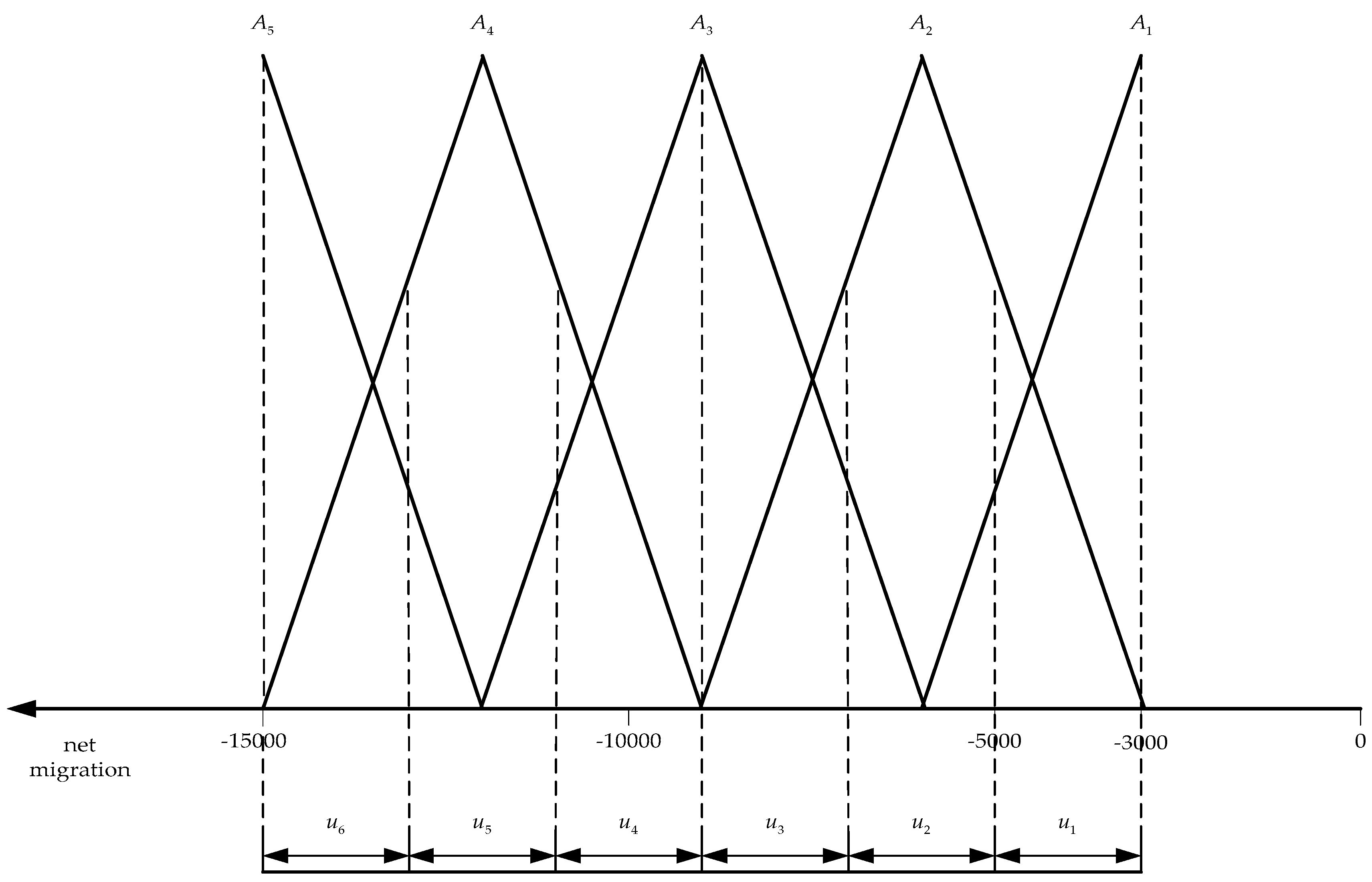
In this work, we use 6 intervals of the same length. These intervals are displayed at the bottom of
Figure 1.
- 3.
Formation of fuzzy linguistic categories.
We form 5 fuzzy linguistic categories
in the operating range. Graphs of membership functions of net migration values to these categories are presented in the upper part of
Figure 1.
In terms of the qualitative meanings of net migration, the fuzzy linguistic categories defined above are interpreted as follows:
—low;
—medium-low;
—medium;
—medium-high;
—high.
- 4.
Fuzzification of deterministic net migration values.
To perform this procedure for each historical net migration value, using the membership function plots in
Figure 1, we define that fuzzy category, the degree of belonging to which this historical value is maximum. For example, the net migration value −11,860 has the maximum degree of membership to the fuzzy linguistic category
. Therefore, the fuzzy category
is taken as the fuzzified value for the given net migration value.
The fuzzified net migration values thus determined are presented in the
column of
Table 1.
Relationships between fuzzy linguistic categories and intervals can be represented in the following form:
- 5.
Set formation of fuzzy logical connectives between fuzzified values of pure migration. These connectives display each consecutive pair of fuzzy linguistic categories from the 5th column of
Table 1.
- 6.
Grouping fuzzy logical connectives.
Let us group the fuzzy logical connectives in such a way that each group has connections the predecessor of which is one fuzzy logical connective. We have:
- 7.
Forecasting values at relevant points in a fuzzy time series.
In [
17], the following algorithm for calculating the forecasted values in the fuzzy time series is proposed.
If the fuzzy historical value at the moment of time is , and there is only one logical connective, for example , and the maximum membership value belongs to the interval , then the value at the midpoint of the interval is taken as the forecasted value at the time .
If there are logical connectives in the group that connect the fuzzy category with the categories , ,... , and the maximum membership values for these categories refer to the intervals ,, ..., , respectively, and the average values of these intervals are , , ..., , then the forecasted value at the moment of time is equal to the average of these values: .
Let the fuzzy value at the time be , and there is no logical connection for . If the maximum membership value for belongs to the interval , then the forecasted value at the moment of time is taken as the value of the midpoint of the interval .
As an example, let us perform calculations for fuzzy linguistic categories and .
- -
fuzzy linguistic category .
There is only one fuzzy logical connective in the corresponding group. Since the fuzzy linguistic category has the maximum degree of membership in the interval , then the forecasted value at the time point following the time point with the linguistic value of net migration equal to , should be taken as the midpoint of the interval : .
- -
fuzzy linguistic category .
There are three fuzzy logical connectives
,
,
in the corresponding group. The fuzzy category
has the maximum degree of membership on the interval
with the midpoint
. The fuzzy category
has the maximum degree of membership exactly on the boundary of the intervals
and
, therefore, we take the midpoint of the common interval as the midpoint:
:
. The fuzzy category
has the maximum degree of membership on the interval
with the midpoint
. The forecasted value at the time point
following the time point with the net migration linguistic value equal to
, is calculated as:
The remaining calculations are performed by analogy. The calculation results are presented in the 6-th column of
Table 1.
In the situation under consideration, a fuzzy linguistic category in 2020 has only one fuzzy logical connective , so the forecast for 2021 will be a fuzzy category . As this category corresponds to the range of net migration values we can forecast that the actual value of net migration in 2021 will be in this interval.
5.2. Forecasting Based on Method2
The second algorithm we use in this article is the one presented in [
23]. A distinctive feature of this method is that it uses a specific partition of the working range of values of the forecasted value into intervals, resulting in intervals of unequal length.
The method presented below involves performing the following procedures:
Using the previously obtained results, we have the following operating range: .
- 2.
Division of the operating range into a certain number of intervals of the same length.
Set the initial number of intervals to 2. We have the following intervals:
;
.
- 3.
Determination the number of data points that fall within each initial interval.
Using the historical data in the 4th column of
Table 1, we have the following distribution of data points over intervals:
interval : 6 data points;
interval : 3 data points.
- 4.
Division of initial intervals into subintervals.
The original paper [
23] recommended dividing the initial interval with the largest number of data points into 4 subintervals of the same length and the interval with the second largest number of data points into 3 subintervals of the same length. Let us divide the first initial interval into 4 subintervals of the same length and the second initial interval into 3 subintervals of the same length. As a result, we have the following set of operating intervals:
with the midpoint ;
with the midpoint ;
with the midpoint ;
with the midpoint ;
with the midpoint ;
with the midpoint ;
with the midpoint .
- 5.
Formation of fuzzy categories.
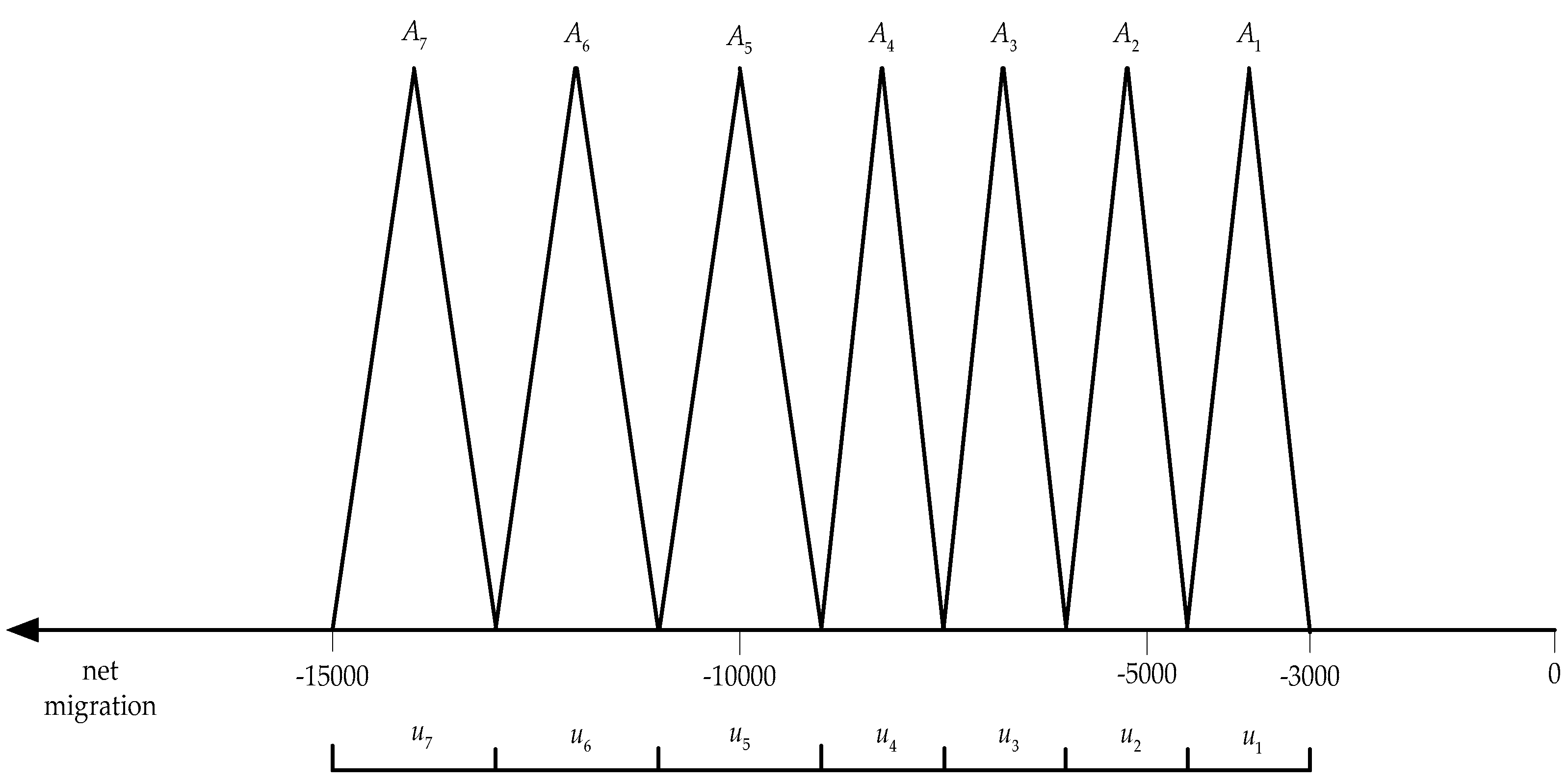
Let us form fuzzy categories on the formed intervals. Let us represent these categories in the form of triangular fuzzy numbers, the graphs of membership functions of which are shown in
Figure 2.
In our case, these fuzzy categories are formally formed on the intervals generated above and have nothing to do with subjective verbal assessments. Therefore, we will simply call them fuzzy categories. If desired, linguistic labels can be assigned to these categories, but this will not change the essence of the fuzzy forecasting method under consideration.
- 6.
Fuzzification of historical data.
Let us restore the historical data on net migration in Latvia in the 2nd column of
Table 2. For each data point, we determine its membership to the corresponding interval. Assign this data point a fuzzy category for this interval. Fuzzified historical data values are presented in the 3rd column of
Table 2.
- 7.
Formation of fuzzy categories groups.
For each of the groups of fuzzy categories in the 3rd column of
Table 2, we form the corresponding group of fuzzy categories based on the following rules:
- -
for an intermediate fuzzy category , the group includes fuzzy categories , , ;
- -
for the first fuzzy category , the group includes fuzzy categories , ;
- -
for the last fuzzy category , the group includes fuzzy categories , .
Groups of fuzzy categories formed on the base of these rules are presented in the 4th column of
Table 2.
- 8.
Calculation of predicted values.
To calculate the forecasted values of fuzzy time series in [
23], possible calculation expressions are used:
where
,
,
interval midpoints for fuzzy categories
,
,
, respectively.
As an example, let us calculate the forecasted value for the fuzzy category
in the first row of
Table 2.
The remaining calculations are performed by analogy. The calculation results are presented in the 5th column of
Table 2.
A feature of this method is that the calculation of the forecasted value is performed at the current point in the time sequence. Therefore, we cannot formally calculate the predicted value of net migration in 2021. Considering that in years 2019 and 2020 the values of net migration were estimated by the fuzzy category , we predict that in 2021 the expected value will also be estimated by the fuzzy category . Turning to numerical values, we can expect a net migration value in the interval .
5.3. Forecasting Based on Method3
This method is proposed in [
25]. The calculation procedures using this method are like to the calculation procedures using Method2. The difference between these methods is as follows: Method2 uses the original historical data as input data, Method3 uses the relative changes in the forecast value between two successive time periods as input data points, expressed as a percentage.
For historical data on net migration in Latvia, these relative changes are presented in the 3rd column of
Table 3. Changes are calculated as follows. Let in a year
the value of net migration be
, and in a year
−
. Then
Calculation of forecasted values of net migration includes the following sequence of procedures.
The maximum negative value of percent change is −39.3, the maximum positive value is 23.0. We have the following initial range: . To simplify subsequent calculations, we form the following operating range: .
- 2.
The initial division of the operating range into intervals.
At this step, we divide the operating range into two initial intervals:
Taking into account the specifics of new forecasted value and the large spread of its values, in order to increase the accuracy of the forecasting results, we form 8 subintervals of the same length in the initial interval and 4 subintervals of the same length in the initial interval . As a result, we have the following set of working intervals:
with the midpoint ;
with the midpoint ;
with the midpoint ;
with the midpoint ;
with the midpoint ;
with the midpoint ;
with the midpoint ;
with the midpoint ;
with the midpoint ;
with the midpoint ;
with the midpoint ;
with the midpoint .
- 3.
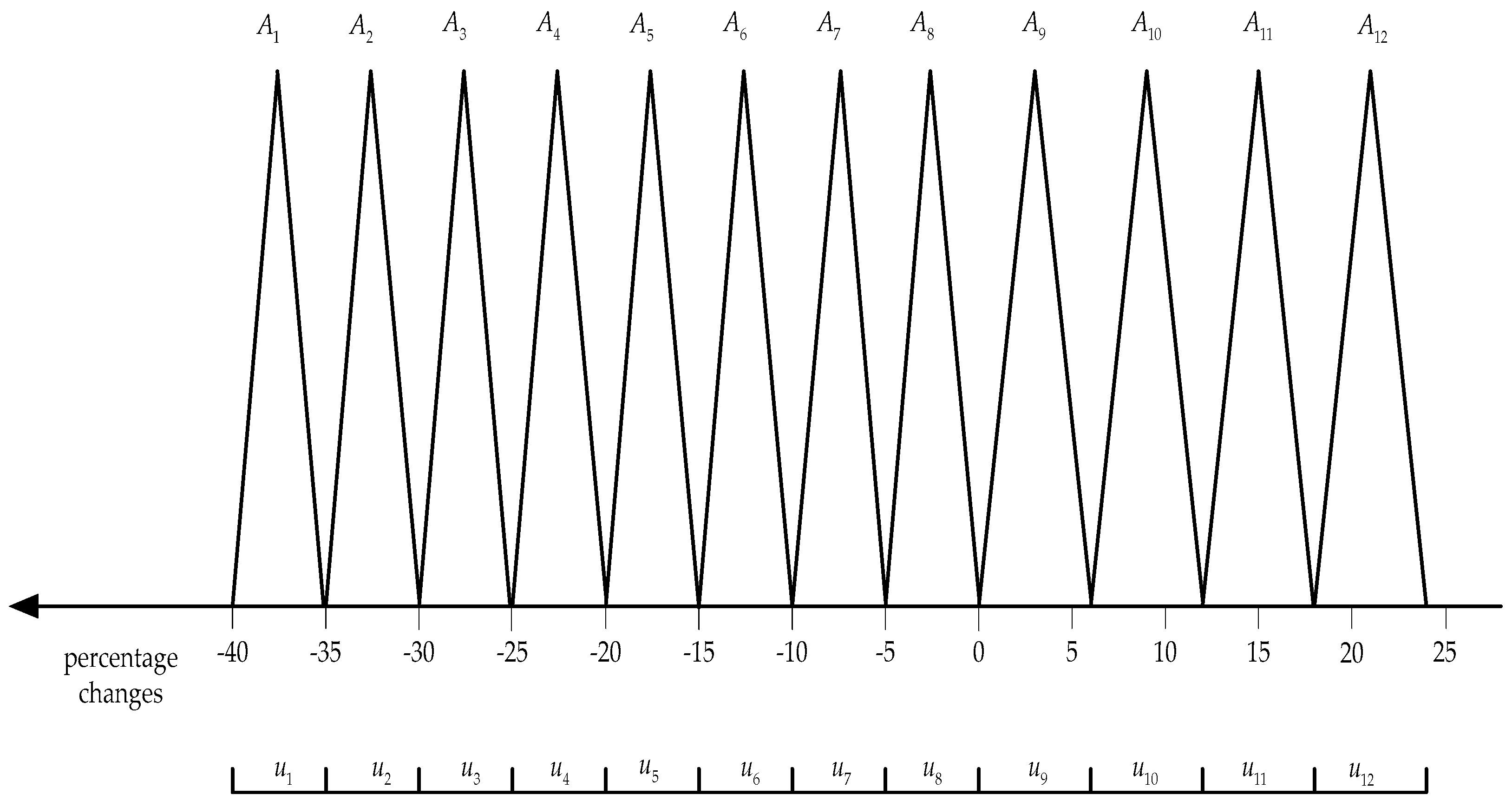
Formation of fuzzy categories.
We form fuzzy categories on each of the intervals of values of new forecasted variable. Let us represent each fuzzy category in the form of a triangular fuzzy number. Graphs of membership functions for all fuzzy categories are shown in
Figure 3.
- 4.
Fuzzification of initial data.
Let us attribute each value of the percentage change to the fuzzy category, in the interval of which the given value falls. Fuzzified change values are presented in the 5th column of
Table 3.
- 5.
Formation of fuzzy categories groups.
This procedure is exactly the same as when using Method2. The formed groups of categories are presented in the 6th column of
Table 3.
- 6.
Forecasting of percentage change values.
The calculation of the relevant predicted values is performed according to the expression (4). As an example, let us provide the calculation of the forecasted value
for the fuzzy category
in the first row of
Table 3.
The remaining calculations are performed by analogy. The calculation results are presented in the 7th column of
Table 3.
- 7.
Prediction of net migration values.
For the current value of net migration in a year
, this value is calculated based on the historical value of net migration in a year
and forecasted percentage change in net migration in a year
relative to the year
. The forecasted net migration values are presented in the 8th column of
Table 3.
How can we forecast the expected value of net migration in 2021? To do this, we assume that the percentage change in net migration relative to 2020 will belong to the fuzzy category , that is, it will be in the interval . From here, we can expect that the actual value of net migration in 2021 will be in the interval .
6. Evaluation and Analysis of Results
Let us evaluate the accuracy of the forecasting results. To do this, for each of the algorithms used, we calculate the absolute deviations
and relative absolute deviations
of the predicted values from the corresponding historical values. The results are presented in
Table 4,
Table 5 and
Table 6.
The largest average relative error occurs when using Method1: 0.31105 or 31%. When using Method2, this error is 0.04502 or 4.5%. The smallest average relative error occurs when using Method3: 0.01841 or 1.8%.
The large value of the average relative error when using Method1 is due to the underlying principle of calculating forecasted values. Let the fuzzy linguistic category of net migration be equal Aj in a year and in a year the fuzzy linguistic category of net migration be equal to . If, in addition to a fuzzy connection , a fuzzy linguistic category has fuzzy logical connectives with fuzzy linguistic categories , then the forecasted value of net migration in a year will depend on the midpoints of all intervals corresponding to fuzzy linguistic categories . If these fuzzy linguistic categories are far from the fuzzy linguistic category on the measurement scale of the forecasted variable, then the estimated forecasted value in the year may be significantly less or greater than its historical value. This leads to large forecasting errors.
This method is very sensitive to sudden changes in historical data values at close time points. The statistics on net migration in Latvia until 2012 are of just such a nature, so in this article, we limited ourselves to data on net migration in 2012–2020.
Chen’s algorithm [
17] was once proposed as an alternative to the original algorithm in [
15,
16,
17] in order to get rid of extremely large calculations. Although this goal has been achieved, the results of forecasting based on this algorithm are rather inaccurate. We used this archaic algorithm in this work only for the purpose of comparing its results with the results given by modern, more accurate algorithms.
It should be noted that Chen’s algorithm is indeed a forecasting method, since a fuzzy linguistic category in a year and its fuzzy logical connections with other fuzzy linguistic categories are used to calculate the predicted value in a year .
When using Method2 [
23], fuzzy categories of forecasted value are formed not in isolation from the intervals defined in the operating range of changes in this value, but directly on these intervals. This greatly simplifies the practical use of the method.
In general, fuzzy linguistic categories, as in Chen’s algorithm, appear to be rather artificial constructions since their main purpose is to link with operating intervals. The relevant calculations use the midpoints of these intervals. The use of fuzzy linguistic categories makes sense if the subjective assessment of historical data is possible only in terms of such categories, for example, the subjective assessment of the quality of weather or the mood of an individual. However, even in such very uncertain conditions, it is necessary to introduce some, for example, a point scale, for measuring a historical variable. This is required by the very essence of Chen’s algorithm.
An essential feature of Method2 is that each forecasted value is calculated at the current time point, so long as in essence, this method is a specific analogue of the method of smoothing deterministic time sequences based on the moving average. Therefore, to forecast the value of the relevant quantity outside the time sequence, some heuristic approach must be used.
The highest accuracy of forecasting results was achieved using Method3 [
25]. The following explanation can be offered for this. At the very beginning of the forecasting process, the original time sequence is transformed into another time sequence, the elements of which are net migration changes at two consecutive time points, expressed as a percentage. The new scale explicitly reflects exactly the successive changes in the original historical data at all time points. This transformation of historical data makes it possible to achieve high forecasting accuracy. Implicitly ignoring such changes in Method1 leads to inaccurate forecasting results.
Except the sensitivity to sudden changes in historical data values at close time points, all three methods give once relatively short-term reliable forecasts. Forecasting results using the first time points of prospect interval leadlead to fast coming the only one value.
In a broader context, all versions of the fuzzy time series forecasting methods proposed in literature use historical enrolment data from Alabama University. The results obtained, which are more accurate than those obtained by other methods, are interpreted by the authors as an advantage of their proposed method.
However, there are relatively few analyses in literature of forecasting parameters influence on the accuracy of its results. These analyses are mainly concerned with the effect of interval lengths on the accuracy of the results. Unfortunately, the authors of the article did not find any source in which a detailed analysis of the impact of sharp changes in the predicted value at various time points on the forecasting accuracy would be given. This problem may become a direction for further research.
7. Discussion
In this article, the fuzzy time series forecasting methods are used to forecast net migration in Latvia. The reason is the high degree of uncertainty in the initial data. These initial data are transformed in the form of linguistic categories. The forecasting procedures are implemented using these linguistic categories. The output data are deterministic numbers. These numbers can be transformed into intervals accordingly to relevant fuzzy categories for input data.
To evaluate and compare the forecasting results, the only criterion used was relative forecasting error; as far as computational complexity of all three methods, it is roughly identical.
Fuzzy time series forecasting methods have undeniable advantages when initial data have a high degree of uncertainty.
However, these methods have an important drawback: they give only short-term forecasts. For migration problems in Latvia, a short-term forecast is sufficient in order to make decisions for migration flow stabilization.
We can use traditional well-known deterministic forecasting methods for migration forecasting and receive deterministic results. These results have low reliability. Therefore, the use of effective fuzzy time series forecasting method for migration forecasting in Latvia seems theoretically and practically well founded.
8. General Conclusions
Using the results received in this work, it can be asserted that the fuzzy methods are suitable for migration flow forecasting in Latvia. This is due to the high degree of uncertainty in migration statistical data. In addition to official migration registration, there are considerable latent migration flows that are not reflected in statistical data. Therefore, the use of fuzzy time series forecasting for migration flows in Latvia seems completely well founded.
This article presents three alternative methods for predicting net migration in Latvia based on a fuzzy time series. In modern historical conditions, negative net migration in Latvia takes place from 1992 to 2020. Until 2012, changes in net migration were irregular and convulsive. In some years, the value of net migration was several times higher than its value in the previous year.
In the last decade, there has been some order in the successive values of net migration. In the last two years, there has been a steady decrease. It can be expected that negative net migration will change its sign to positive in the coming years. However, for this, the following conditions must be met: (1) an increase in the well-being of population in Latvia, which will lead to an increase in the flow of re-emigrants to Latvia; (2) for migration flow, the government needs to provide favorable conditions for residents of Latvia which should guarantee a high living level; and (3) more active involvement of workers and specialists from other countries.


