

Mid-Infrared Emissivity Retrieval from Nighttime Sentinel-3 SLSTR Images Combining Split-Window Algorithms and the Radiance Transfer Method


Abstract
1. Introduction
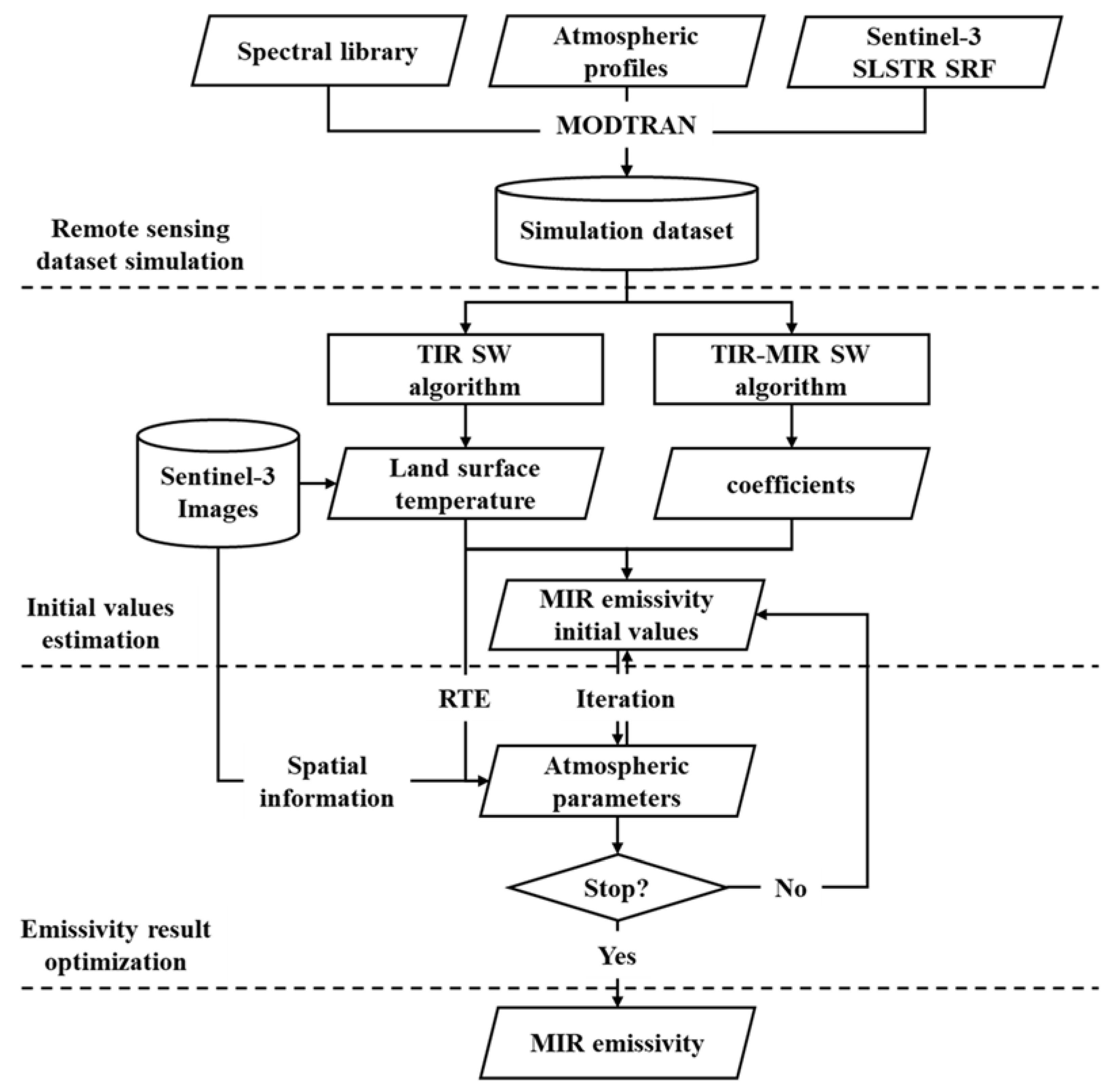
2. Data and Method
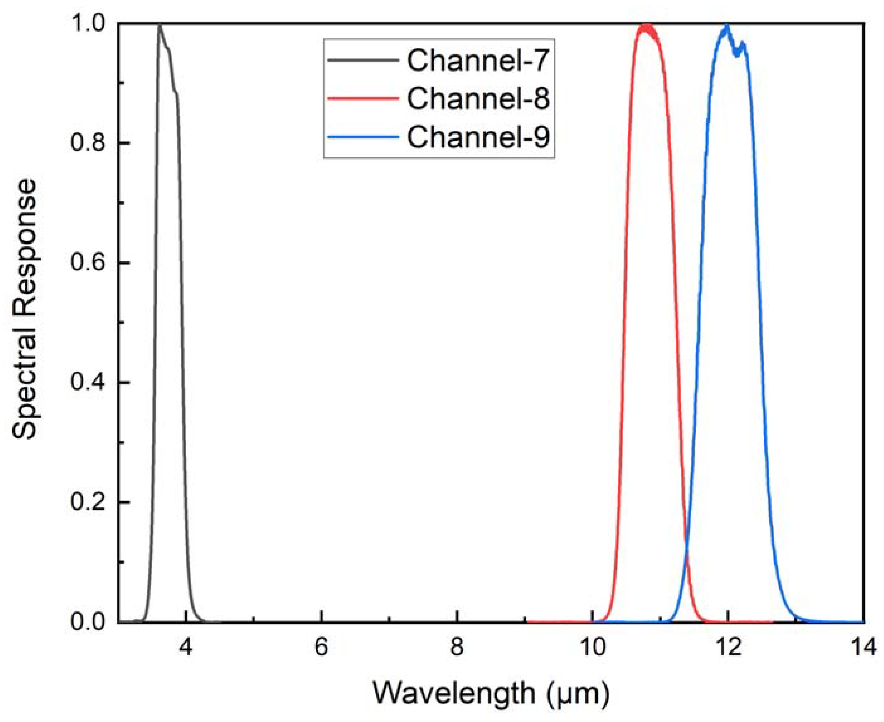
2.1. Remote Sensing Dataset Simulation
2.2. Initial Values Estimation
2.2.1. Development of SW Algorithms
2.2.2. MIR Emissivity Estimation
2.3. Emissivity Result Optimization
3. Experimental Results
3.1. Retrieval of the Simulation Dataset
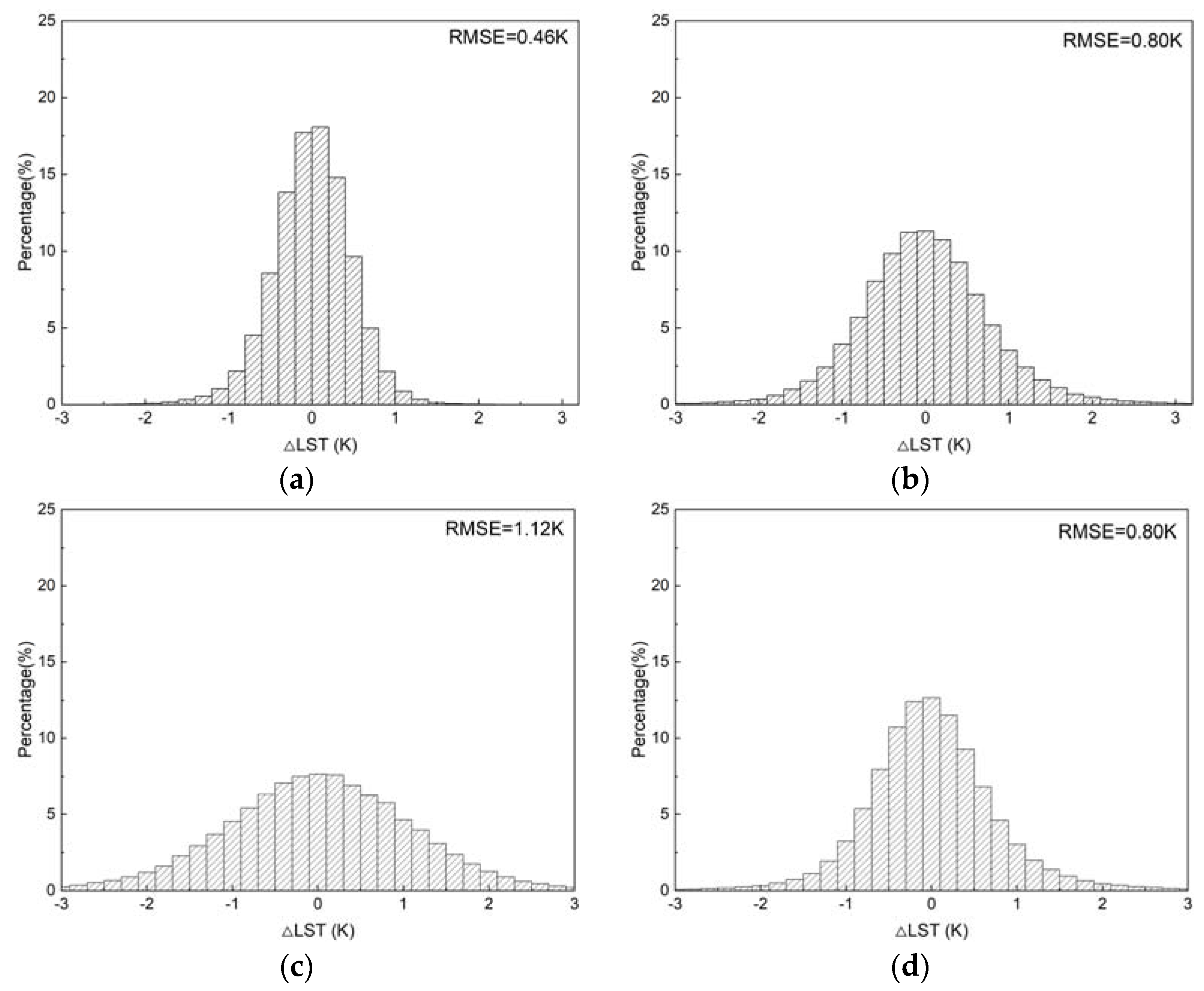
3.1.1. LST Retrieval Results
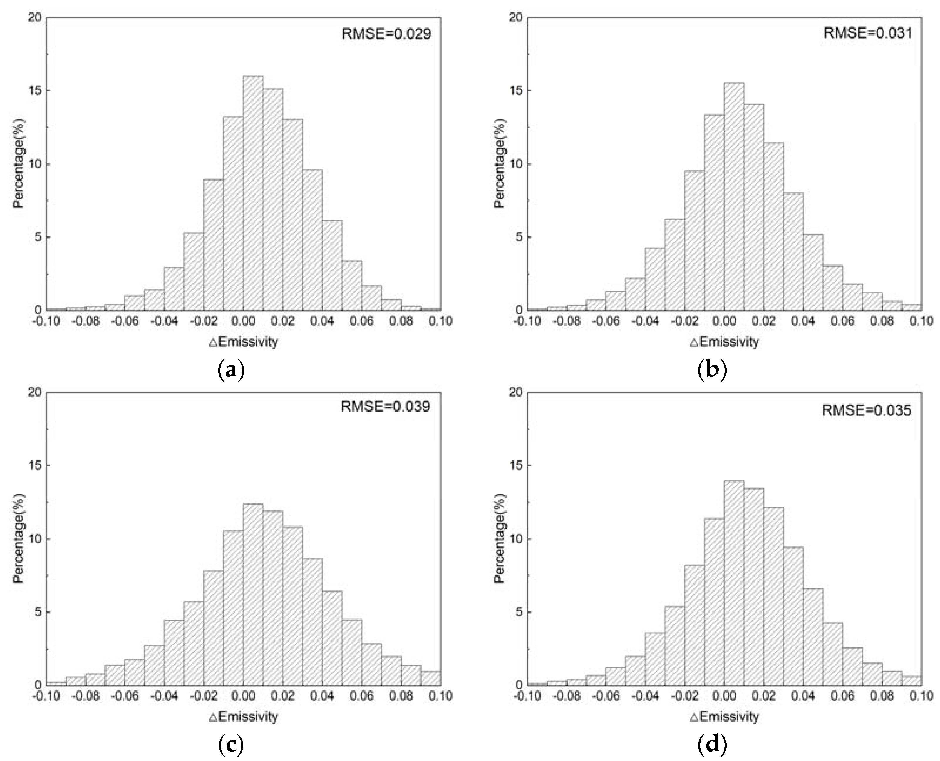
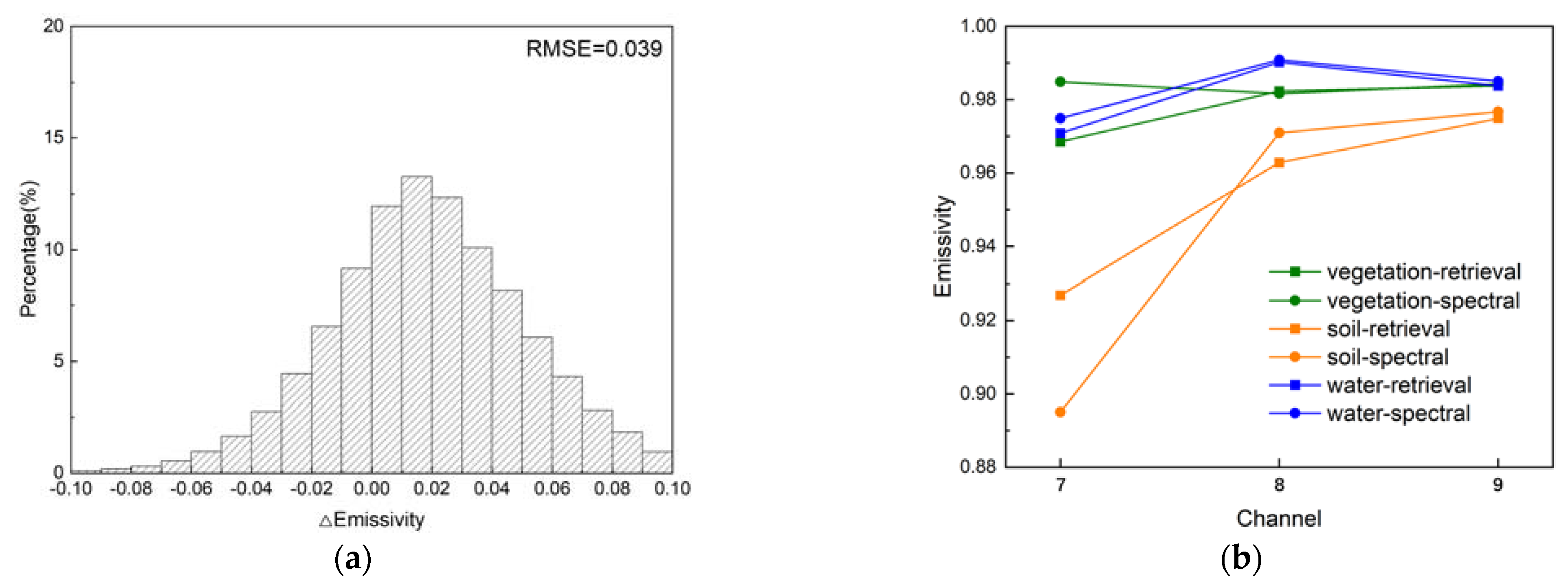
3.1.2. MIR Emissivity Results
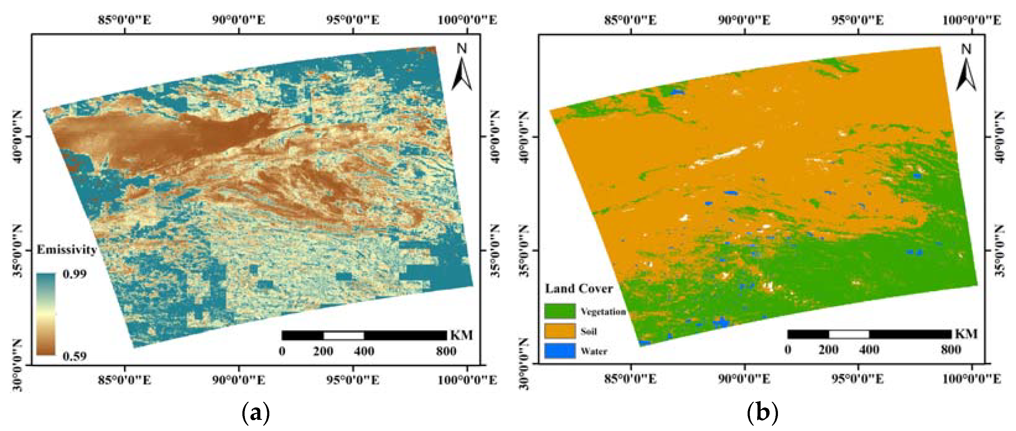
3.2. Sentinel-3 SLSTR Images Application
4. Discussions
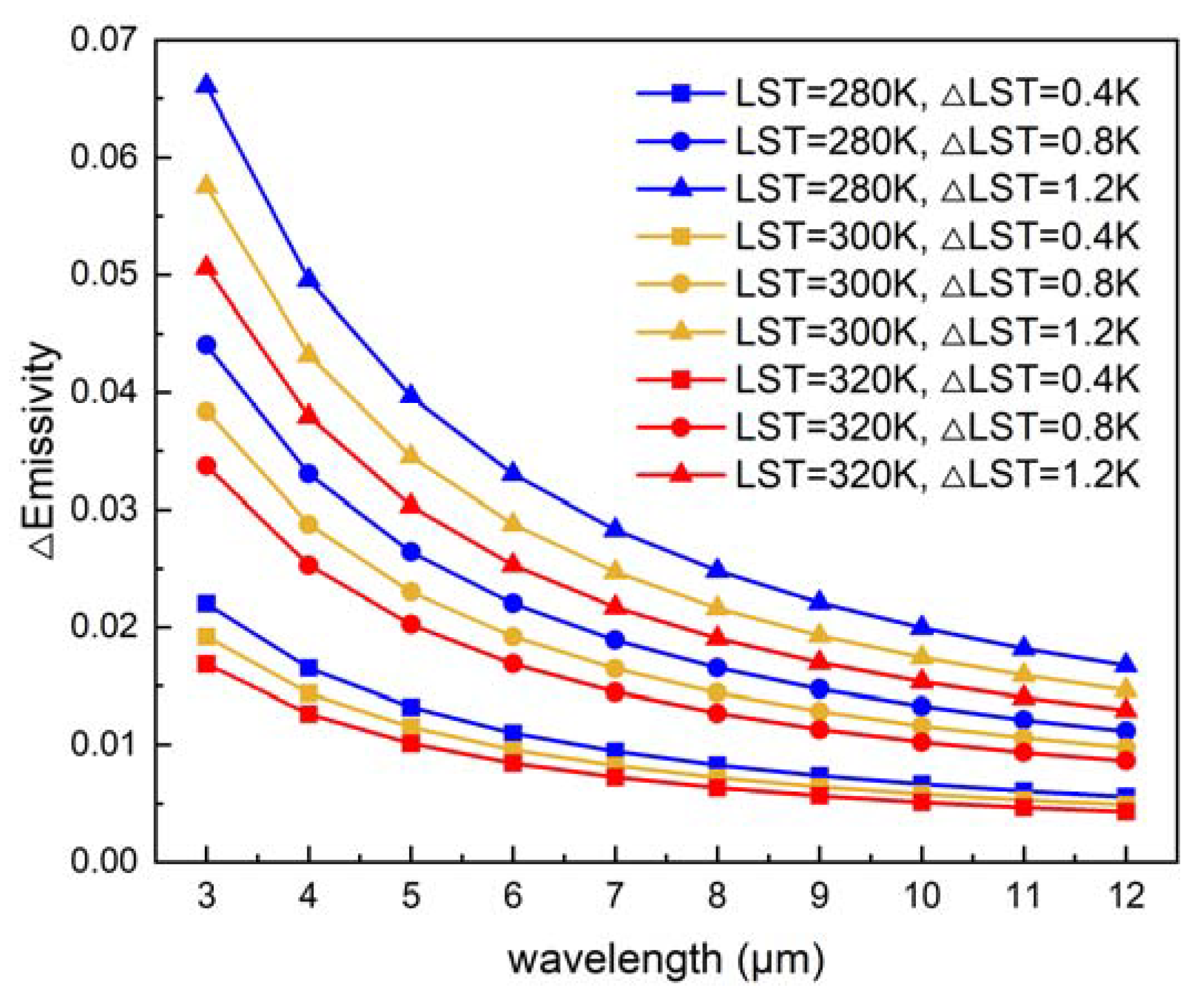
4.1. Relationship between the Errors of LSTs and Emissivity
4.2. Future Improvements of the Proposed Method
5. Conclusions
Author Contributions
Funding
Institutional Review Board Statement
Informed Consent Statement
Data Availability Statement
Acknowledgments
Conflicts of Interest
References
- Tang, B.-H.; Shao, K.; Li, Z.-L.; Wu, H.; Tang, R. An improved NDVI-based threshold method for estimating land surface emissivity using MODIS satellite data. Int. J. Remote Sens. 2015, 36, 4864–4878. [Google Scholar] [CrossRef]
- Xu, H.; Xu, D.; Chen, S.; Ma, W.; Shi, Z. Rapid Determination of Soil Class Based on Visible-Near Infrared, Mid-Infrared Spectroscopy and Data Fusion. Remote Sens. 2020, 12, 1512. [Google Scholar] [CrossRef]
- Boyd, D.S.; Wicks, T.E.; Curran, P.J. Use of middle infrared radiation to estimate the leaf area index of a boreal forest. Tree Physiol. 2000, 20, 755–760. [Google Scholar] [CrossRef] [PubMed]
- Boyd, D.S.; Duane, W.J. Exploring spatial and temporal variation in middle infrared reflectance (at 3.75 @m) measured from the tropical forests of west Africa. Int. J. Remote Sens. 2001, 22, 1861–1878. [Google Scholar] [CrossRef]
- Adab, H.; Kanniah, K.D.; Solaimani, K. Modeling forest fire risk in the northeast of Iran using remote sensing and GIS techniques. Natural Hazards 2012, 65, 1723–1743. [Google Scholar] [CrossRef]
- Qian, Y.G.; Wang, N.; Ma, L.L.; Liu, Y.K.; Wu, H.; Tang, B.H.; Tang, L.L.; Li, C.R. Land surface temperature retrieved from airborne multispectral scanner mid-infrared and thermal-infrared data. Opt. Express 2016, 24, A257–A269. [Google Scholar] [CrossRef]
- Tang, B.-H.; Wang, J. A Physics-Based Method to Retrieve Land Surface Temperature From MODIS Daytime Midinfrared Data. IEEE Trans. Geosci. Remote Sens. 2016, 54, 4672–4679. [Google Scholar] [CrossRef]
- Zheng, Y.; Ren, H.; Guo, J.; Ghent, D.; Tansey, K.; Hu, X.; Nie, J.; Chen, S. Land Surface Temperature Retrieval from Sentinel-3A Sea and Land Surface Temperature Radiometer, Using a Split-Window Algorithm. Remote Sens. 2019, 11, 650. [Google Scholar] [CrossRef]
- Qian, Y.-G.; Zhao, E.-Y.; Gao, C.; Wang, N.; Ma, L. Land Surface Temperature Retrieval Using Nighttime Mid-Infrared Channels Data From Airborne Hyperspectral Scanner. IEEE J. Sel. Top. Appl. Earth Obs. Remote Sens. 2015, 8, 1208–1216. [Google Scholar] [CrossRef]
- Libonati, R.; DaCamara, C.; Setzer, A.; Morelli, F.; Melchiori, A. An Algorithm for Burned Area Detection in the Brazilian Cerrado Using 4 µm MODIS Imagery. Remote Sens. 2015, 7, 15782–15803. [Google Scholar] [CrossRef]
- Li, Z.-L.; Wu, H.; Wang, N.; Qiu, S.; Sobrino, J.A.; Wan, Z.; Tang, B.-H.; Yan, G. Land surface emissivity retrieval from satellite data. Int. J. Remote Sens. 2013, 34, 3084–3127. [Google Scholar] [CrossRef]
- Jiang, G.-M.; Li, Z.-L. Intercomparison of two BRDF models in the estimation of the directional emissivity in MIR channel from MSG1-SEVIRI data. Opt. Express 2008, 16, 19310–19321. [Google Scholar] [CrossRef] [PubMed]
- Tang, B.-H.; Li, Z.-L.; Bi, Y. Estimation of land surface directional emissivity in mid-infrared channel around 4.0 μm from MODIS data. Opt. Express 2009, 17, 3173–3182. [Google Scholar]
- Becker, F.; Li, Z.-L. Temperature-Independent Spectral Indices in Thermal Infrared Bands. Remote Sens. Environ. 1990, 32, 17–33. [Google Scholar] [CrossRef]
- Françoise, N.; François, P.; Marc Philippe, S. Bidirectional Reflectivity in AVHRR Channel 3: Application to a Region in Northern Africa. Remote Sens. Environ. 1998, 66, 298–316. [Google Scholar] [CrossRef]
- Nie, J.; Ren, H.; Zheng, Y.; Ghent, D.; Tansey, K. Land Surface Temperature and Emissivity Retrieval From Nighttime Middle-Infrared and Thermal-Infrared Sentinel-3 Images. IEEE Geosci. Remote Sens. Lett. 2020, 18, 915–919. [Google Scholar] [CrossRef]
- Zeng, H.; Ren, H.; Nie, J.; Zhu, J.; Ye, X.; Jiang, C. Land Surface Temperature and Emissivity Retrieval from Nighttime Middle and Thermal Infrared Images of Chinese Fengyun-3D MERSI-II. IEEE J. Sel. Top. Appl. Earth Obs. Remote Sens. 2021, 14, 7724–7733. [Google Scholar] [CrossRef]
- Tang, B.-H.; Li, Z.-L. Retrieval of land surface bidirectional reflectivity in the mid-infrared from MODIS channels 22 and 23. Int. J. Remote Sens. 2008, 29, 4907–4925. [Google Scholar] [CrossRef]
- Li, Z.-L.; Becker, F. Feasibility of land surface temperature and emissivity determination from AVHRR data. Remote Sens. Environ. 1993, 43, 67–85. [Google Scholar] [CrossRef]
- Li, Z.-L.; Petitcolin, F.; Zhang, R. A physically based algorithm for land surface emissivity retrieval from combined mid-infrared and thermal infrared data. Sci. China Ser. E: Technol. Sci. 2000, 43, 23–33. [Google Scholar] [CrossRef]
- Gillespie, A.; Rokugawa, S.; Matsunaga, T.; Cothern, J.S.; Hook, S.; Kahle, A.B. A Temperature and Emissivity Separation Algorithm for Advanced Spaceborne Thermal Emission and Reflection Radiometer (ASTER) Images. IEEE Trans. Geosci. Remote Sens. 1998, 36, 1113–1126. [Google Scholar] [CrossRef]
- Li, Z.-L.; Tang, B.-H.; Wu, H.; Ren, H.; Yan, G.; Wan, Z.; Trigo, I.F.; Sobrino, J.A. Satellite-derived land surface temperature: Current status and perspectives. Remote Sens. Environ. 2013, 131, 14–37. [Google Scholar] [CrossRef]
- Ye, X.; Ren, H.; Liu, R.; Qin, Q.; Liu, Y.; Dong, J. Land Surface Temperature Estimate From Chinese Gaofen-5 Satellite Data Using Split-Window Algorithm. IEEE Trans. Geosci. Remote Sens. 2017, 55, 5877–5888. [Google Scholar] [CrossRef]
- Ren, H.; Liu, R.; Qin, Q.; Fan, W.; Yu, L.; Du, C. Mapping finer-resolution land surface emissivity using Landsat images in China. J. Geophys. Res. Atmos. 2017, 122, 6764–6781. [Google Scholar] [CrossRef]
- Baldridge, A.M.; Hook, S.J.; Grove, C.I.; Rivera, G. The ASTER spectral library version 2.0. Remote Sens. Environ. 2009, 113, 711–715. [Google Scholar] [CrossRef]
- William, C.S.; Wan, Z.; Zhang, Y.; Feng, Y. Thermal Infrared (3–14 μm) bidirectional reflectance measurements of sands and soils. Remote Sens. Environ. 1997, 60, 101–109. [Google Scholar] [CrossRef]
- Chevallier, F.; Chéruy, F.; Scott, N.A.; Chédin, A. A Neural Network Approach for a Fast and Accurate Computation of a Longwave Radiative Budget. J. Appl. Meteorol. 1998, 37, 1385–1397. [Google Scholar] [CrossRef]
- Ye, X.; Ren, H.; Zhu, J.; Fan, W.; Qin, Q. Split-Window Algorithm for Land Surface Temperature Retrieval From Landsat-9 Remote Sensing Images. IEEE Geosci. Remote Sens. Lett. 2022, 19, 7507205. [Google Scholar] [CrossRef]
- Wan, Z. New refinements and validation of the collection-6 MODIS land-surface temperature/emissivity product. Remote Sens. Environ. 2014, 140, 36–45. [Google Scholar] [CrossRef]
- Becker, F.; Li, Z.-L. Towards a local split window method over land surfaces. Int. J. Remote Sens. 1990, 11, 369–393. [Google Scholar] [CrossRef]
- Wan, Z.; Dozier, J. A generalized split-window algorithm for retrieving land-surface temperature from space. IEEE Trans. Geosci. Remote Sens. 1996, 34, 892–905. [Google Scholar] [CrossRef]
- Du, C.; Ren, H.; Qin, Q.; Meng, J.; Zhao, S. A Practical Split-Window Algorithm for Estimating Land Surface Temperature from Landsat 8 Data. Remote Sens. 2015, 7, 647–665. [Google Scholar] [CrossRef]
- Ye, X.; Ren, H.; Liang, Y.; Zhu, J.; Guo, J.; Nie, J.; Zeng, H.; Zhao, Y.; Qian, Y. Cross-calibration of Chinese Gaofen-5 thermal infrared images and its improvement on land surface temperature retrieval. Int. J. Appl. Earth Obs. Geoinf. 2021, 101, 102357. [Google Scholar] [CrossRef]
- Duan, S.-B.; Li, Z.-L.; Li, H.; Göttsche, F.-M.; Wu, H.; Zhao, W.; Leng, P.; Zhang, X.; Coll, C. Validation of Collection 6 MODIS land surface temperature product using in situ measurements. Remote Sens. Environ. 2019, 225, 16–29. [Google Scholar] [CrossRef]
- Sun, D.; Pinker, R.T. Estimation of land surface temperature from a Geostationary Operational Environmental Satellite (GOES-8). J. Geophys. Res. 2003, 108, 4326. [Google Scholar] [CrossRef]
- Caselles, E.; Valor, E.; Abad, F.; Caselles, V. Automatic classification-based generation of thermal infrared land surface emissivity maps using AATSR data over Europe. Remote Sens. Environ. 2012, 124, 321–333. [Google Scholar] [CrossRef]
- Zhang, S.; Duan, S.-B.; Li, Z.-L.; Huang, C.; Wu, H.; Han, X.-J.; Leng, P.; Gao, M. Improvement of Split-Window Algorithm for Land Surface Temperature Retrieval from Sentinel-3A SLSTR Data Over Barren Surfaces Using ASTER GED Product. Remote Sens. 2019, 11, 3025. [Google Scholar] [CrossRef]
- Coppo, P.; Ricciarelli, B.; Brandani, F.; Delderfield, J.; Ferlet, M.; Mutlow, C.; Munro, G.; Nightingale, T.; Smith, D.; Bianchi, S.; et al. SLSTR: A high accuracy dual scan temperature radiometer for sea and land surface monitoring from space. J. Mod. Opt. 2010, 57, 1815–1830. [Google Scholar] [CrossRef]
- Kanani, K.; Poutier, L.; Nerry, F.; Stoll, M.P. Directional Effects Consideration to Improve out-doors Emissivity Retrieval in the 3–13 µm Domain. Opt. Express 2007, 15, 12464–12482. [Google Scholar] [CrossRef]
- Cheng, J.; Liang, S.; Liu, Q.; Li, X. Temperature and emissivity separation from ground-based MIR hyperspectral data. IEEE Trans. Geosci. Remote Sens. 2011, 49, 1473–1484. [Google Scholar] [CrossRef]
- Ren, H.; Yan, G.; Chen, L.; Li, Z. Angular effect of MODIS emissivity products and its application to the split-window algorithm. ISPRS J. Photogramm. Remote Sens. 2011, 66, 498–507. [Google Scholar] [CrossRef]
- Zheng, X.; Li, Z.-L.; Wang, T.; Huang, H.; Nerry, F. Determination of global land surface temperature using data from only five selected thermal infrared channels: Method extension and accuracy assessment. Remote Sens. Environ. 2022, 268, 112774. [Google Scholar] [CrossRef]
- Ren, H.; Ye, X.; Liu, R.; Dong, J.; Qin, Q. Improving Land Surface Temperature and Emissivity Retrieval From the Chinese Gaofen-5 Satellite Using a Hybrid Algorithm. IEEE Trans. Geosci. Remote Sens. 2018, 56, 1080–1090. [Google Scholar] [CrossRef]
- Ren, H.; Dong, J.; Liu, R.; Zheng, Y.; Guo, J.; Chen, S.; Nie, J.; Zhao, Y. New hybrid algorithm for land surface temperature retrieval from multiple-band thermal infrared image without atmospheric and emissivity data inputs. Int. J. Digital Earth 2020, 13, 1430–1453. [Google Scholar] [CrossRef]
- Zhao, E.; Qian, Y.; Gao, C.; Huo, H.; Jiang, X.; Kong, X. Land Surface Temperature Retrieval Using Airborne Hyperspectral Scanner Daytime Mid-Infrared Data. Remote Sens. 2014, 6, 12667–12685. [Google Scholar] [CrossRef]
- Ren, H.; Du, C.; Liu, R.; Qin, Q.; Yan, G.; Li, Z.-L.; Meng, J. Atmospheric water vapor retrieval from Landsat 8 thermal infrared images. J. Geophys. Res. Atmos. 2015, 120, 1723–1738. [Google Scholar] [CrossRef]


| Channel | c | e1 | e2 | e3 | e4 | e5 | e6 | RMSE |
|---|---|---|---|---|---|---|---|---|
| 7 | 1.0043 | −0.2230 | −1.0291 | 1.3553 | −0.2443 | 0.2590 | −0.9229 | 0.0572 |
| 8 | 0.9368 | 0.0721 | −0.2294 | 0.1593 | −0.0179 | 0.0646 | 0.0009 | 0.0174 |
| 9 | 0.9638 | 0.0674 | −0.2542 | 0.2387 | −0.0861 | 0.0369 | 0.0051 | 0.0085 |
| SW Algorithm | Polar | Mid-Latitude | Tropical | Overall |
|---|---|---|---|---|
| TIR | 0.46 | 0.80 | 1.12 | 0.80 |
| MIR-TIR | 0.44 | 0.70 | 0.89 | 0.75 |
| MIR Emissivity | Polar | Mid-Latitude | Tropical | Overall |
|---|---|---|---|---|
| Initial values | 0.053 | 0.045 | 0.048 | 0.055 |
| Optimized results | 0.029 | 0.031 | 0.039 | 0.035 |
Disclaimer/Publisher’s Note: The statements, opinions and data contained in all publications are solely those of the individual author(s) and contributor(s) and not of MDPI and/or the editor(s). MDPI and/or the editor(s) disclaim responsibility for any injury to people or property resulting from any ideas, methods, instructions or products referred to in the content. |
© 2022 by the authors. Licensee MDPI, Basel, Switzerland. This article is an open access article distributed under the terms and conditions of the Creative Commons Attribution (CC BY) license (https://creativecommons.org/licenses/by/4.0/).
Share and Cite
Ye, X.; Ren, H.; Wang, P.; Sun, Z.; Zhu, J. Mid-Infrared Emissivity Retrieval from Nighttime Sentinel-3 SLSTR Images Combining Split-Window Algorithms and the Radiance Transfer Method. Int. J. Environ. Res. Public Health 2023, 20, 37. https://doi.org/10.3390/ijerph20010037
Ye X, Ren H, Wang P, Sun Z, Zhu J. Mid-Infrared Emissivity Retrieval from Nighttime Sentinel-3 SLSTR Images Combining Split-Window Algorithms and the Radiance Transfer Method. International Journal of Environmental Research and Public Health. 2023; 20(1):37. https://doi.org/10.3390/ijerph20010037
Chicago/Turabian StyleYe, Xin, Huazhong Ren, Pengxin Wang, Zhongqiu Sun, and Jian Zhu. 2023. "Mid-Infrared Emissivity Retrieval from Nighttime Sentinel-3 SLSTR Images Combining Split-Window Algorithms and the Radiance Transfer Method" International Journal of Environmental Research and Public Health 20, no. 1: 37. https://doi.org/10.3390/ijerph20010037
APA StyleYe, X., Ren, H., Wang, P., Sun, Z., & Zhu, J. (2023). Mid-Infrared Emissivity Retrieval from Nighttime Sentinel-3 SLSTR Images Combining Split-Window Algorithms and the Radiance Transfer Method. International Journal of Environmental Research and Public Health, 20(1), 37. https://doi.org/10.3390/ijerph20010037