
Impact of “Three Red Lines” Water Policy (2011) on Water Usage Efficiency, Production Technology Heterogeneity, and Determinant of Water Productivity Change in China


Abstract
1. Introduction
2. Literature Review
2.1. Water Usage Efficiency and Regional Production Technology Heterogeneity
2.2. Water Usage Total Factor Productivity and Its Determinants
3. Methodology
3.1. Super-Efficiency SBM Model with Undesirable Outputs
3.2. DEA Meta-Frontier Model
3.3. Malmquist–Luenberger Index
3.4. Mann–Whitney U and Kruskal–Wallis Tests
4. Inputs-Outputs Selection and Data Sources
5. Results and Discussion
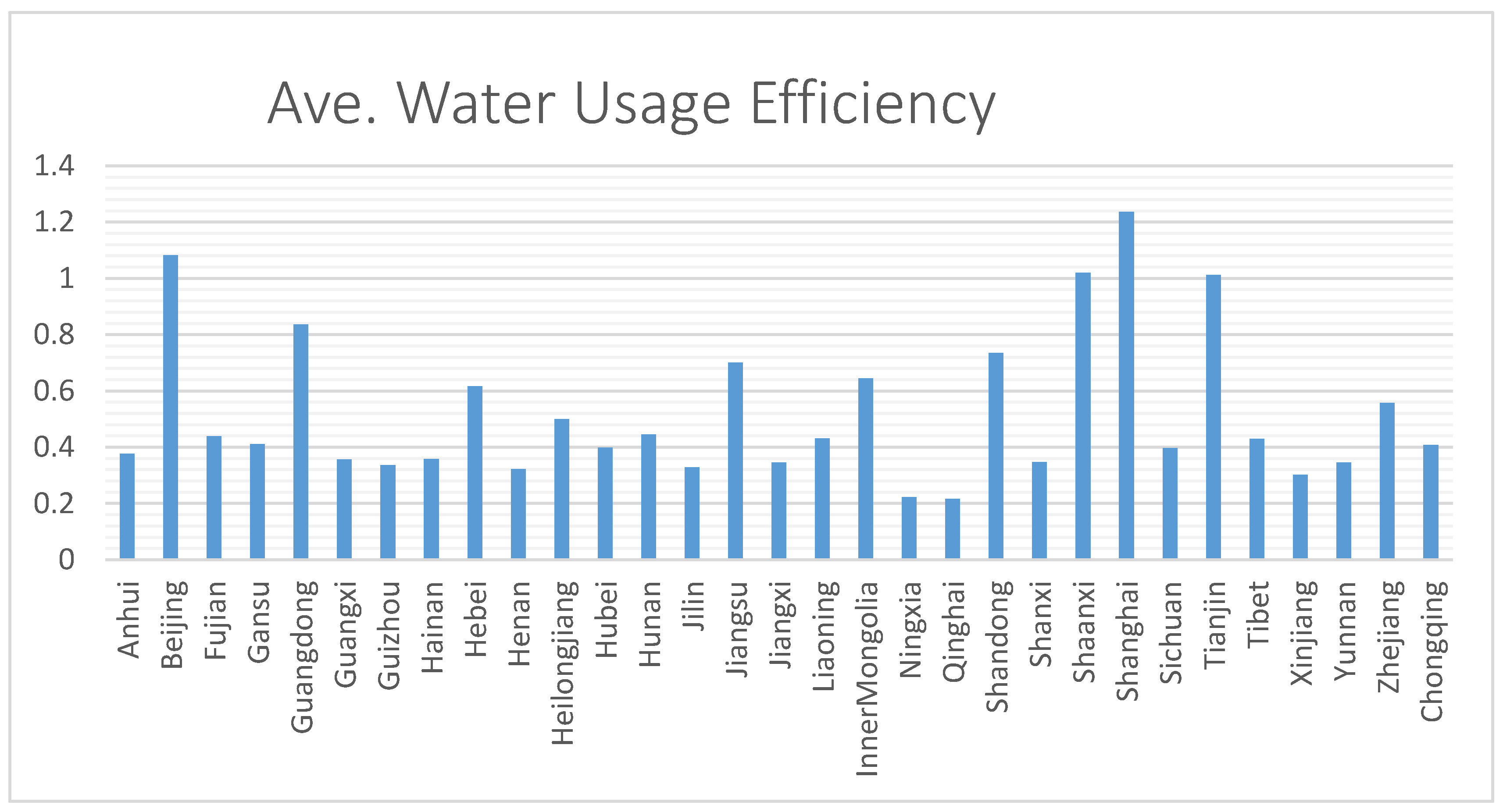
5.1. SBM-DEA Results
5.2. Meta-Frontier DEA Results
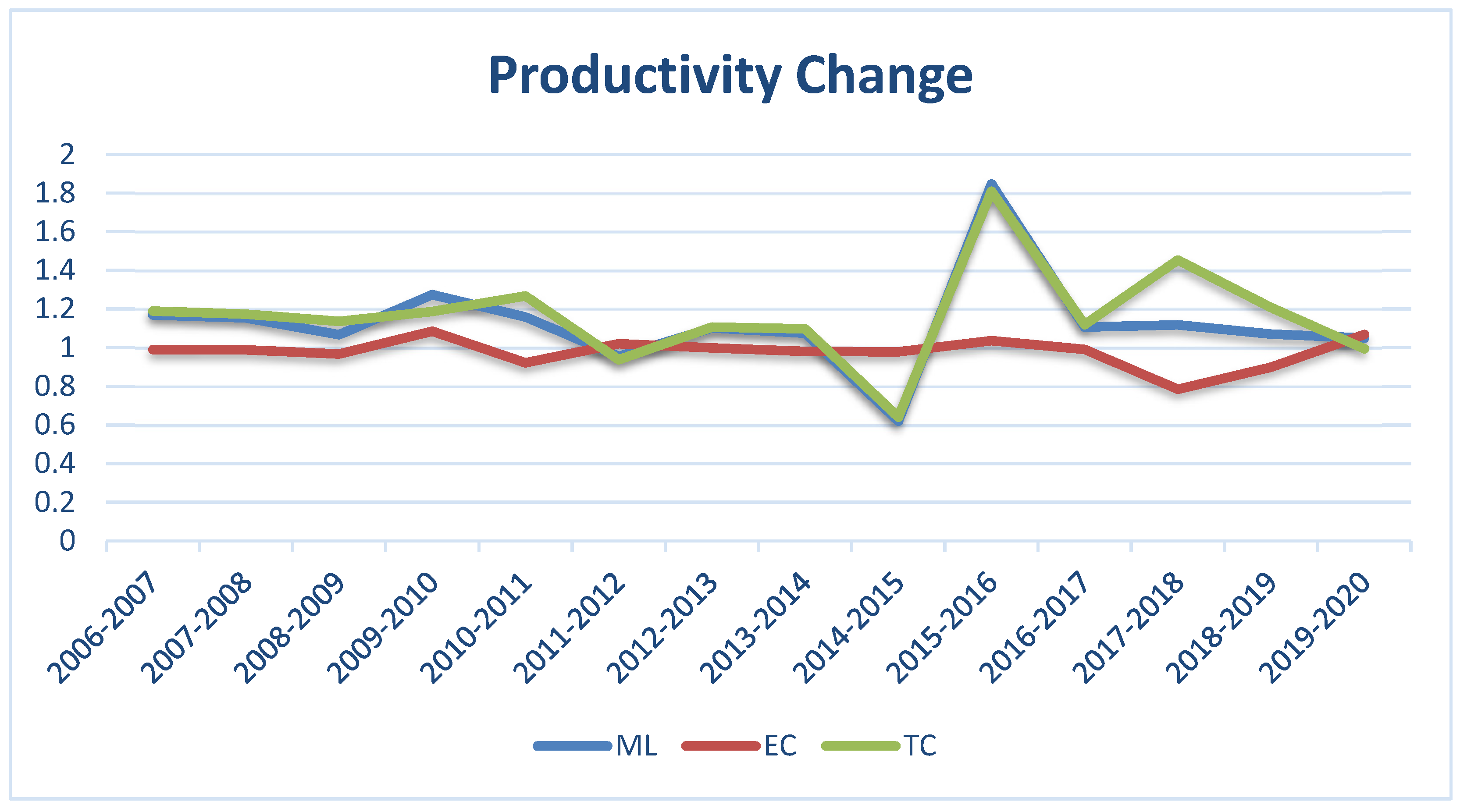
5.3. Malmquist–Luenberger Index Results
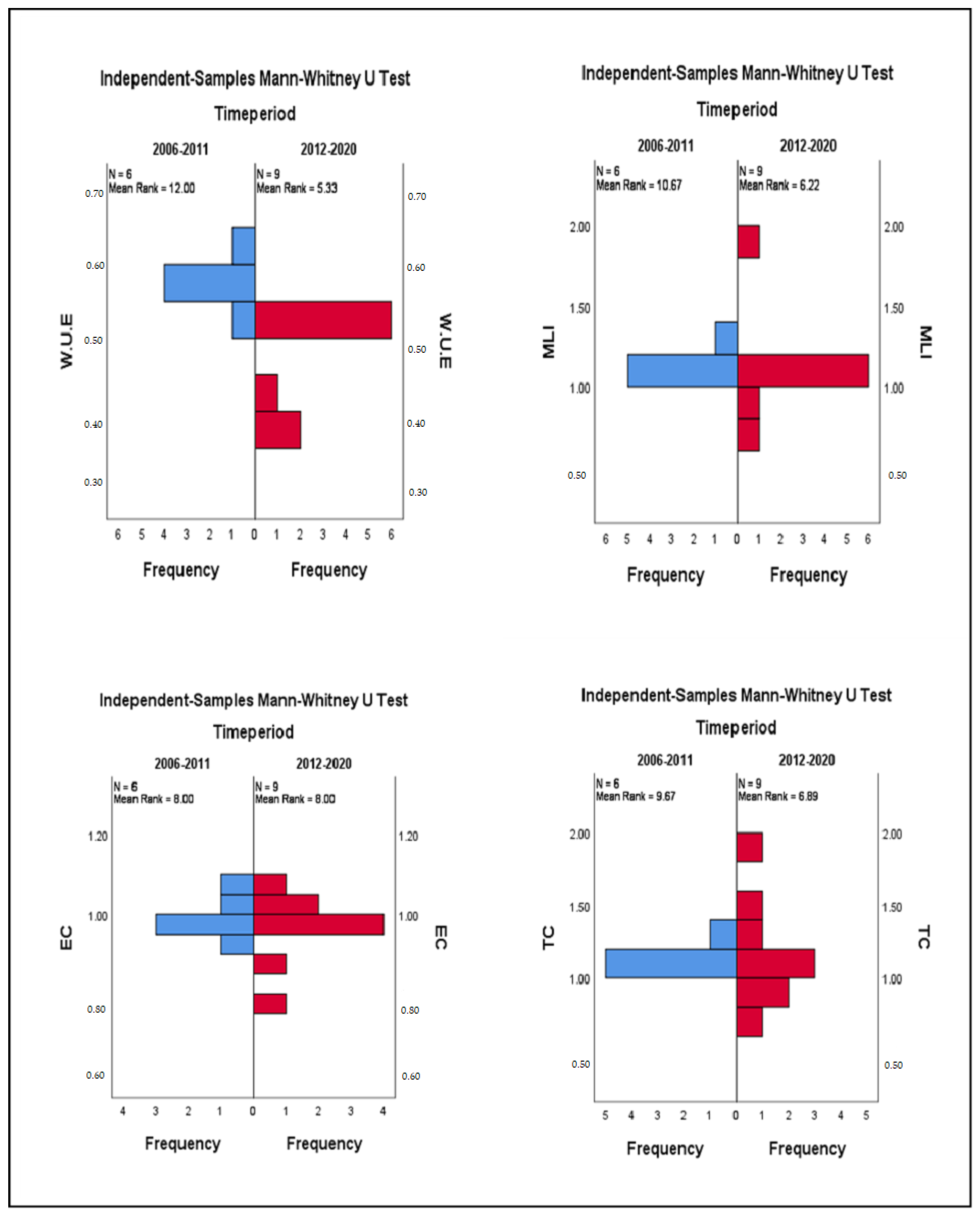
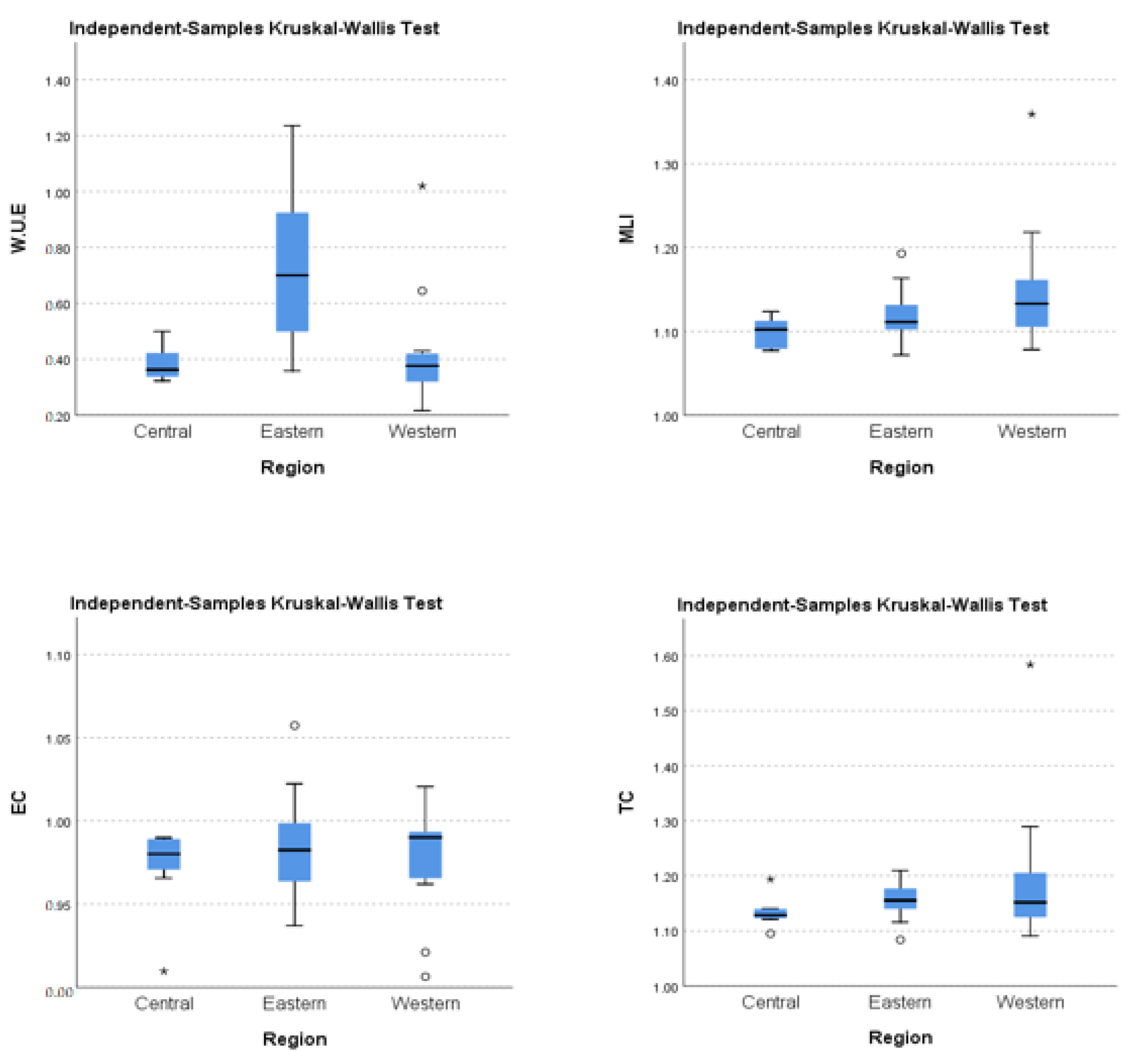
5.4. Mann–Whitney U and Kruskal–Wallis Test Results
6. Conclusions and Recommendations
Author Contributions
Funding
Institutional Review Board Statement
Informed Consent Statement
Data Availability Statement
Acknowledgments
Conflicts of Interest
Appendix A

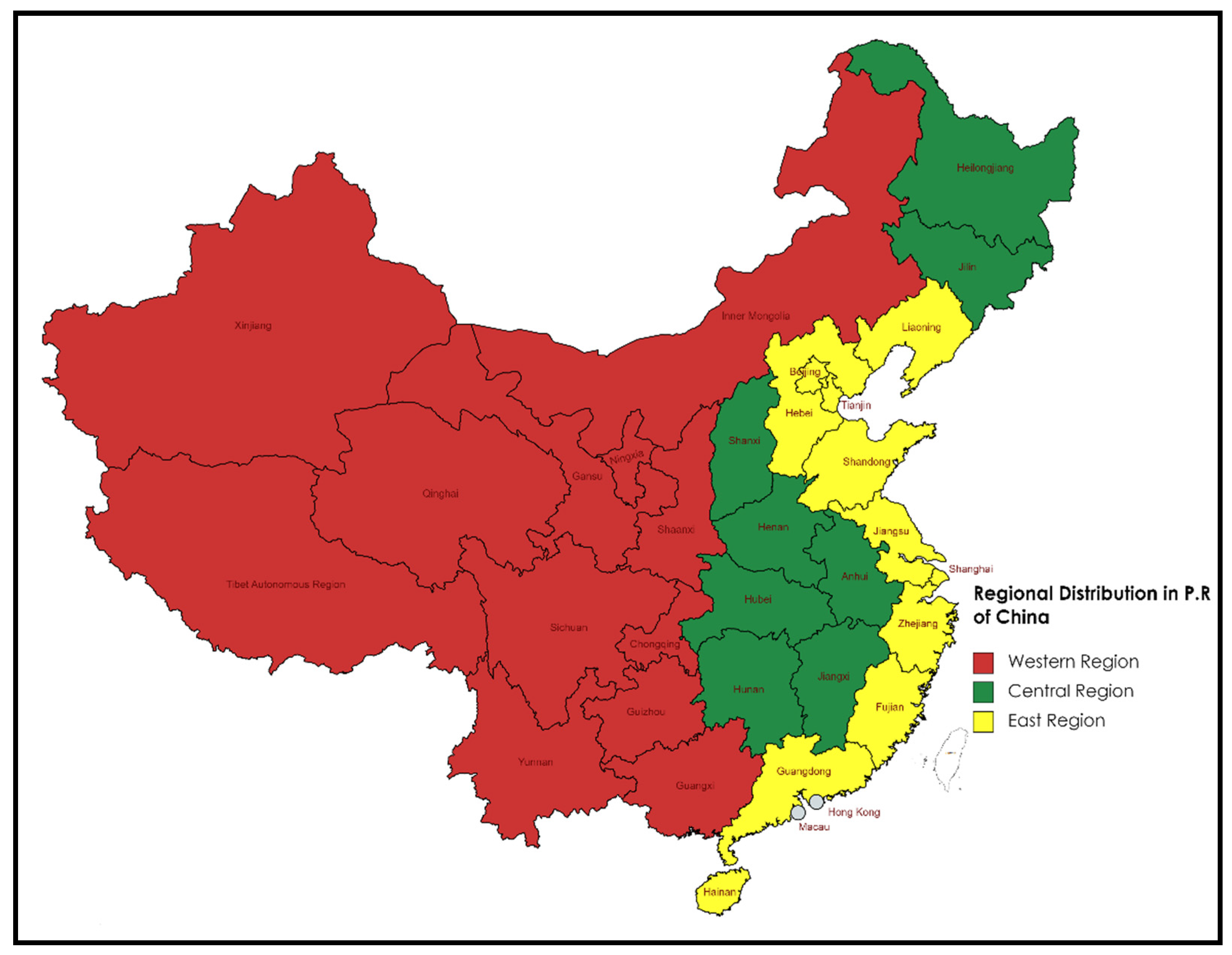
| East | Central | West |
|---|---|---|
| Beijing | Anhui | Gansu |
| Fujian | Henan | Guangxi |
| Guangdong | Heilongjiang | Guizhou |
| Hainan | Hubei | Inner Mongolia |
| Hebei | Hunan | Ningxia |
| Jiangsu | Jilin | Qinghai |
| Liaoning | Jiangxi | Shaanxi |
| Shandong | Shanxi | Sichuan |
| Shanghai | Tibet | |
| Tianjin | Xinjiang | |
| Zhejiang | Yunnan | |
| Chongqing |
| Year | East | Central | West |
|---|---|---|---|
| 2006 | 0.7959 | 0.4784 | 0.5273 |
| 2007 | 0.8019 | 0.4668 | 0.4988 |
| 2008 | 0.7876 | 0.4159 | 0.5256 |
| 2009 | 0.7857 | 0.3894 | 0.4661 |
| 2010 | 0.8414 | 0.4499 | 0.4328 |
| 2011 | 0.7511 | 0.3989 | 0.4203 |
| 2012 | 0.7424 | 0.3949 | 0.4457 |
| 2013 | 0.7475 | 0.3949 | 0.4395 |
| 2014 | 0.7341 | 0.3841 | 0.438 |
| 2015 | 0.8017 | 0.3698 | 0.4085 |
| 2016 | 0.7286 | 0.3906 | 0.4113 |
| 2017 | 0.7342 | 0.3899 | 0.3987 |
| 2018 | 0.6167 | 0.2893 | 0.3247 |
| 2019 | 0.4999 | 0.2626 | 0.3088 |
| 2020 | 0.5504 | 0.274 | 0.3164 |
| Avg. | 0.7279 | 0.3833 | 0.4242 |
| Year | East | Central | West |
|---|---|---|---|
| 2006 | 0.7968 | 0.7183 | 0.8995 |
| 2007 | 0.8022 | 0.7976 | 0.9073 |
| 2008 | 0.7876 | 0.8146 | 0.88 |
| 2009 | 0.7879 | 0.9444 | 0.852 |
| 2010 | 0.8461 | 0.9317 | 0.8688 |
| 2011 | 0.7557 | 0.9839 | 0.8015 |
| 2012 | 0.7453 | 0.985 | 0.7634 |
| 2013 | 0.7502 | 0.9618 | 0.7978 |
| 2014 | 0.7367 | 0.9535 | 0.7799 |
| 2015 | 0.8042 | 0.9399 | 0.7763 |
| 2016 | 0.7299 | 0.9267 | 0.7745 |
| 2017 | 0.7543 | 0.8924 | 0.8454 |
| 2018 | 0.6488 | 0.7938 | 0.8609 |
| 2019 | 0.5392 | 0.768 | 0.8788 |
| 2020 | 0.5504 | 0.7735 | 0.8552 |
| Avg. | 0.7357 | 0.879 | 0.8361 |

References
- Wu, J. Challenges for Safe and Healthy Drinking Water in China. Curr. Environ. Health Rep. 2020, 7, 292–302. [Google Scholar] [CrossRef] [PubMed]
- Jiang, Y. Economics of Water Scarcity in China. In Oxford Research Encyclopedia of Environmental Science; Oxford University Press: Oxford, UK, 2020. [Google Scholar] [CrossRef]
- Li, Y.; Shen, J.; Lu, L.; Luo, Y.; Wang, L.; Shen, M. Water environmental stress, rebound effect, and economic growth of China’s textile industry. PeerJ 2018, 6, e5112. [Google Scholar] [CrossRef] [PubMed]
- Yuan, B.; Li, C.; Xiong, X. Innovation and environmental total factor productivity in China: The moderating roles of economic policy uncertainty and marketization process. Environ. Sci. Pollut. Res. 2021, 28, 9558–9581. [Google Scholar] [CrossRef] [PubMed]
- China Water Use, Resources and Precipitation—Worldometer. Available online: https://www.worldometers.info/water/china-water/ (accessed on 9 October 2022).
- He, C.; Harden, C.P.; Liu, Y. Comparison of water resources management between China and the United States. Geogr. Sustain. 2020, 1, 98–108. [Google Scholar] [CrossRef]
- China Water Resources Bulletin 2011—Hydropower Knowledge Network. China Water Resources and Hydropower Press. Available online: http://waterpub.com.cn/shop/detail_523458.html (accessed on 9 October 2022).
- Me-Nsope, N.; Larkins, M. Regional and Sectoral Impacts of Water Redline Policy in China: Results from an Integrated Regional CGE Water Model. J. Gend. Agric. Food Secur. 2016, 1, 1–22. [Google Scholar]
- Emrouznejad, A.; Yang, G.L. A survey and analysis of the first 40 years of scholarly literature in DEA: 1978–2016. Socio-Econ. Plan. Sci. 2018, 61, 4–8. [Google Scholar] [CrossRef]
- Shah, W.U.H.; Hao, G.; Yasmeen, R.; Kamal, M.A.; Khan, A.; Padda, I.U.H. Unraveling the role of China’s OFDI, institutional difference and B&R policy on energy efficiency: A meta-frontier super-SBM approach. Environ. Sci. Pollut. Res. 2022, 29, 56454–56472. [Google Scholar] [CrossRef]
- Xu, T.; You, J.; Li, H.; Shao, L. Energy efficiency evaluation based on data envelopment analysis: A literature review. Energies 2020, 13, 3548. [Google Scholar] [CrossRef]
- di Liu, K.; Yang, G.L.; Yang, D.G. Industrial water-use efficiency in China: Regional heterogeneity and incentives identification. J. Clean. Prod. 2020, 258, 120828. [Google Scholar] [CrossRef]
- Wang, J.F.; Zhang, T.L.; Fu, B.J. A measure of spatial stratified heterogeneity. Ecol. Indic. 2016, 67, 250–256. [Google Scholar] [CrossRef]
- Azad, M.A.S.; Ancev, T.; Hernández-Sancho, F. Efficient Water Use for Sustainable Irrigation Industry. Water Resour. Manag. 2015, 29, 1683–1696. [Google Scholar] [CrossRef]
- Amit Kumar, T.K.T.; Mishra, S.; Bakshi, S.; Upadhyay, P. Response of eutrophication and water quality drivers on greenhouse gas emissions in lakes of China: A critical analysis. Ecohydrology 2022, e2483. [Google Scholar] [CrossRef]
- Kumar, A.; Palmate, S.S.; Shukla, R. Water Quality Modelling, Monitoring, and Mitigation. Appl. Sci. 2022, 12, 11403. [Google Scholar] [CrossRef]
- Hu, J.L.; Wang, S.C.; Yeh, F.Y. Total-factor water efficiency of regions in China. Resour. Policy 2006, 31, 217–230. [Google Scholar] [CrossRef]
- Rahman, M.T.; Nielsen, R.; Khan, M.A. Agglomeration externalities and technical efficiency: An empirical application to the pond aquaculture of Pangas and Tilapia in Bangladesh. Aquac. Econ. Manag. 2019, 23, 158–187. [Google Scholar] [CrossRef]
- Xu, H.; Yang, R.; Song, J. Agricultural water use efficiency and rebound effect: A study for China. Int. J. Environ. Res. Public Health 2021, 18, 7151. [Google Scholar] [CrossRef]
- Veettil, P.C.; Speelman, S.; van Huylenbroeck, G. Estimating the Impact of Water Pricing on Water Use Efficiency in Semi-arid Cropping System: An Application of Probabilistically Constrained Non-parametric Efficiency Analysis. Water Resour. Manag. 2013, 27, 55–73. [Google Scholar] [CrossRef]
- Guerrini, A.; Romano, G.; Campedelli, B. Economies of Scale, Scope, and Density in the Italian Water Sector: A Two-Stage Data Envelopment Analysis Approach. Water Resour. Manag. 2013, 27, 4559–4578. [Google Scholar] [CrossRef]
- Manjunatha, A.V.; Speelman, S.; Chandrakanth, M.G.; van Huylenbroeck, G. Impact of groundwater markets in India on water use efficiency: A data envelopment analysis approach. J. Environ. Manag. 2011, 92, 2924–2929. [Google Scholar] [CrossRef]
- Lombardi, G.V.; Stefani, G.; Paci, A.; Becagli, C.; Miliacca, M.; Gastaldi, M.; Giannetti, B.F. CMVB Almeida, The sustainability of the Italian water sector: An empirical analysis by DEA. J. Clean. Prod. 2019, 227, 1035–1043. [Google Scholar] [CrossRef]
- Zhao, F.; Wu, Y.; Ma, S.; Lei, X.; Liao, W. Increased Water Use Efficiency in China and Its Drivers During 2000–2016. Ecosystems 2022, 1–17. [Google Scholar] [CrossRef]
- Pan, Z.; Wang, Y.; Zhou, Y.; Wang, Y. Analysis of the water use efficiency using super-efficiency data envelopment analysis. Appl. Water Sci. 2020, 10, 139. [Google Scholar] [CrossRef]
- Deng, G.; Li, L.; Song, Y. Provincial water use efficiency measurement and factor analysis in China: Based on SBM-DEA model. Ecol. Indic. 2016, 69, 12–18. [Google Scholar] [CrossRef]
- Molinos-Senante, M.; Maziotis, A. Drivers of productivity change in water companies: An empirical approach for England and Wales. Int. J. Water Resour. Dev. 2020, 36, 972–991. [Google Scholar] [CrossRef]
- Zhong, S.; Li, A.; Wu, J. The total factor productivity index of freshwater aquaculture in China: Based on regional heterogeneity. Environ. Sci. Pollut. Res. 2022, 29, 15664–15680. [Google Scholar] [CrossRef]
- Ji, J.; Wang, P. Research on China’s aquaculture efficiency evaluation and influencing factors with undesirable outputs. J. Ocean Univ. China 2015, 14, 569–574. [Google Scholar] [CrossRef]
- Molinos-Senante, M.; Maziotis, A.; Sala-Garrido, R. Assessment of the Total Factor Productivity Change in the English and Welsh Water Industry: A Färe-Primont Productivity Index Approach. Water Resour. Manag. 2017, 31, 2389–2405. [Google Scholar] [CrossRef]
- Maziotis, A.; Sala-Garrido, R.; Mocholi-Arce, M.; Molinos-Senante, M. Total factor productivity assessment of water and sanitation services: An empirical application including quality of service factors. Environ. Sci. Pollut. Res. 2021, 28, 37818–37829. [Google Scholar] [CrossRef]
- Oulmane, A.; Chebil, A.; Frija, A.; Benmehaia, M.A. Water-Saving Technologies and Total Factor Productivity Growth in Small Horticultural Farms in Algeria. Agric. Res. 2020, 9, 585–591. [Google Scholar] [CrossRef]
- Luo, Y.; Yin, L.; Qin, Y.; Wang, Z.; Gong, Y. Evaluating water use efficiency in China’s western provinces based on a slacks-based measure (SBM)-undesirable window model and a malmquist productivity index. Symmetry 2018, 10, 301. [Google Scholar] [CrossRef]
- Koehuan, J.E.; Suharto, B.; Djoyowasito, G.; Susanawati, L.D. Water total factor productivity growth of rice and corn crops using data envelopment analysis—Malmquist index (West timor, indonesia). Agric. Eng. Int. CIGR J. 2020, 22, 20–30. [Google Scholar]
- Goh, K.H.; See, K.F. Measuring the productivity growth of Malaysia’s water sector: Implications for regulatory reform. Util. Policy 2021, 71, 101198. [Google Scholar] [CrossRef]
- Li, T.; Shi, Z.; Han, D. Research on the impact of energy technology innovation on total factor ecological efficiency. Environ. Sci. Pollut. Res. 2022, 29, 37096–37114. [Google Scholar] [CrossRef] [PubMed]
- Song, M.; Peng, L.; Shang, Y.; Zhao, X. Green technology progress and total factor productivity of resource-based enterprises: A perspective of technical compensation of environmental regulation. Technol. Forecast. Soc. Chang. 2022, 174, 121276. [Google Scholar] [CrossRef]
- Tone, K. A slacks-based measure of super-efficiency in data envelopment analysis. Eur. J. Oper. Res. 2002, 204, 694–697. [Google Scholar] [CrossRef]
- Tone, K. Dealing with Undesirable Outputs in DEA: A Slacks-Based Measure (SBM) Approach; GRIPS Research Report Series; GRIPS: Tokyo, Japan, 2003. [Google Scholar]
- Wang, N.; Chen, J.; Yao, S.; Chang, Y.C. A meta-frontier DEA approach to efficiency comparison of carbon reduction technologies on project level. Renew. Sustain. Energy Rev. 2018, 82, 2606–2612. [Google Scholar] [CrossRef]
- Hang, Y.; Sun, J.; Wang, Q.; Zhao, Z.; Wang, Y. Measuring energy inefficiency with undesirable outputs and technology heterogeneity in Chinese cities. Econ. Model. 2015, 49, 46–52. [Google Scholar] [CrossRef]
- Chiu, C.R.; Lu, K.H.; Tsang, S.S.; Chen, Y.F. Decomposition of meta-frontier inefficiency in the two-stage network directional distance function with quasi-fixed inputs. Int. Trans. Oper. Res. 2013, 20, 595–611. [Google Scholar] [CrossRef]
- Chung, Y.H.; Färe, R.; Grosskopf, S. Productivity and undesirable outputs: A directional distance function approach. J. Environ. Manag. 1997, 51, 229–240. [Google Scholar] [CrossRef]
- Mann, H.B.; Whitney, D.R. On a Test of Whether one of Two Random Variables is Stochastically Larger than the Other. Ann. Math. Stat. 1947, 18, 50–60. [Google Scholar] [CrossRef]
- Wilcoxon, F. Individual Comparisons by Ranking Methods. Biom. Bull. 1945, 1, 80–83. [Google Scholar] [CrossRef]
- Theodorsson-Norheim, E. Kruskal-Wallis test: BASIC computer program to perform non-parametric one-way analysis of variance and multiple comparisons on ranks of several independent samples. Comput. Methods Programs Biomed. 1986, 23, 57–62. [Google Scholar] [CrossRef] [PubMed]
- Peyrache, A.; Rose, C.; Sicilia, G. Variable selection in Data Envelopment Analysis. Eur. J. Oper. Res. 2020, 282, 644–659. [Google Scholar] [CrossRef]
- Tone, K. Dealing with undesirable outputs in DEA: A Slacks-Based Measure (SBM) approach. Oper. Res. Soc. Jpn. 2004, 44–45. [Google Scholar]
- Byrnes, J.; Crase, L.; Dollery, B.; Villano, R. The relative economic efficiency of urban water utilities in regional New South Wales and Victoria. Resour. Energy Econ. 2010, 32, 439–455. [Google Scholar] [CrossRef]
- Ali, M.K.; Klein, K.K. Water Use Efficiency and Productivity of the Irrigation Districts in Southern Alberta. Water Resour. Manag. 2014, 28, 2751–2766. [Google Scholar] [CrossRef]
- Linderson, M.L.; Iritz, Z.; Lindroth, A. The effect of water availability on stand-level productivity, transpiration, water use efficiency and radiation use efficiency of field-grown willow clones. Biomass Bioenergy 2007, 31, 460–468. [Google Scholar] [CrossRef]
- Chen, L.; Huang, Y.; Li, M.J.; Wang, Y.M. Meta-frontier analysis using cross-efficiency method for performance evaluation. Eur. J. Oper. Res. 2020, 280, 219–229. [Google Scholar] [CrossRef]
- Kang, L.; Wu, C.; Liao, X.; Wang, B. Safety performance and technology heterogeneity in China’s provincial construction industry. Saf. Sci. 2020, 121, 83–92. [Google Scholar] [CrossRef]
- Wang, R.M.; Tian, Z.; Ren, F.R. Energy efficiency in China: Optimization and comparison between hydropower and thermal power. Energy Sustain. Soc. 2021, 11, 36. [Google Scholar] [CrossRef]
- Wang, S.; Wang, H.; Zhang, L.; Dang, J. Provincial carbon emissions efficiency and its influencing factors in China. Sustainability 2019, 11, 2355. [Google Scholar] [CrossRef]
- Bwambale, E.; Abagale, F.K.; Anornu, G.K. Smart irrigation monitoring and control strategies for improving water use efficiency in precision agriculture: A review. Agric. Water Manag. 2022, 260, 107324. [Google Scholar] [CrossRef]
- Ding, N.; Liu, J.; Yang, J.; Lu, B. Water footprints of energy sources in China: Exploring options to improve water efficiency. J. Clean. Prod. 2018, 174, 1021–1031. [Google Scholar] [CrossRef]
- Kumar, A.; Mishra, S.; Taxak, A.K.; Pandey, R.; Yu, Z.G. Nature rejuvenation: Long-term (1989–2016) vs short-term memory approach based appraisal of water quality of the upper part of Ganga River. India. Environ. Technol. Innov. 2020, 20, 101164. [Google Scholar] [CrossRef]
- Zhang, Y.; Li, X.; Song, Y.; Jiang, F. Can green industrial policy improve total factor productivity? Firm-level evidence from China. Struct. Change Econ. Dyn. 2021, 59, 51–62. [Google Scholar] [CrossRef]
- Zhang, H.; Huang, L.; Zhu, Y.; Si, H.; He, X. Does low-carbon city construction improve total factor productivity? Evidence from a quasi-natural experiment in China. Int. J. Environ. Res. Public Health 2021, 18, 11974. [Google Scholar] [CrossRef]
- Fan, H.; Tao, S.; Hashmi, S.H. Does the construction of a water ecological civilization city improve green total factor productivity? Evidence from a quasi-natural experiment in China. Int. J. Environ. Res. Public Health 2021, 18, 11829. [Google Scholar] [CrossRef]
- Manouseli, D.; Kayaga, S.M.; Kalawsky, R. Evaluating the Effectiveness of Residential Water Efficiency Initiatives in England: Influencing Factors and Policy Implications. Water Resour. Manag. 2019, 33, 2219–2238. [Google Scholar] [CrossRef]
- Zaini, F.M.; Kwong, Q.J.; Jack, L.B. Water efficiency in Malaysian commercial buildings: A green initiative and cost–benefit approach. Int. J. Build. Pathol. Adapt. 2021, 39, 702–719. [Google Scholar] [CrossRef]
- Cheng, L.; Song, S.; Xie, Y. Evaluation of Water Resources Utilization Efficiency in Guangdong Province Based on the DEA–Malmquist Model. Front. Environ. Sci. 2022, 17, 819693. [Google Scholar] [CrossRef]
- Song, M.; Wang, R.; Zeng, X. Water resources utilization efficiency and influence factors under environmental restrictions. J. Clean. Prod. 2018, 184, 611–621. [Google Scholar] [CrossRef]
- Lu, W.; Liu, W.; Hou, M.; Deng, Y.; Deng, Y.; Zhou, B.; Zhao, K. Spatial-temporal evolution characteristics and influencing factors of agriculturalwater use efficiency in northwest China-based on a super-DEA model and a spatial panel econometric model. Water 2021, 13, 632. [Google Scholar] [CrossRef]
- Liu, X.; Han, X.; Zhang, X.; Wang, X.; Yang, L.; Chang, Z.; Liu, H. Using SEBAL Model and HJ Satellite Data to Calculate Regional Evapotranspiration and Irrigation Water Use Efficiency. J. Irrig. Drain. 2021, 40, 136–144. [Google Scholar] [CrossRef]
- Abu-Sharar, T.M.; Al-Karablieh, E.K.; Haddadin, M.J. Role of Virtual Water in Optimizing Water Resources Management in Jordan. Water Resour. Manag. 2012, 26, 3977–3993. [Google Scholar] [CrossRef]
- Xu, R.; Wu, Y.; Wang, G.; Zhang, X.; Wu, W.; Xu, Z. Evaluation of industrial water use efficiency considering pollutant discharge in China. PLoS ONE 2019, 6, e20592. [Google Scholar] [CrossRef] [PubMed]
- Zhang, W.; Du, X.; Huang, A.; Yin, H. Analysis and comprehensive evaluation of water use efficiency in China. Water 2019, 11, 2620. [Google Scholar] [CrossRef]
- Liu, Y.; Geng, J.; Zhang, L.; Jiang, X.; Fu, Y.; Lin, L. Analysis of Agricultural Water Use Efficiency in Shandong Province Based on DEA and Malmquist Model. IOP Conf. Ser. Earth Environ. Sci. 2020, 585, 012090. [Google Scholar] [CrossRef]
- Wang, S.; Tian, N.; Dai, Y.; Duan, H. Measurement of Resource Environmental Performance of Crop Planting Water Consumption Based on Water Footprint and Data Enveloped Analysis. Water Resour. Manag. 2022, 36, 641–658. [Google Scholar] [CrossRef]
- Zhou, X.; Xue, Z.; Seydehmet, J. An empirical study on industrial eco-efficiency in arid resource exploitation region of northwest China. Environ. Sci. Pollut. Res. 2021, 28, 53394–53411. [Google Scholar] [CrossRef]
- Yu, K.; Ying, J.; Gong, R.; Chang, Z. Preliminary discussion of agricultural cost effectiveness evaluation with drip irrigation. Custos E Agronegocio 2021, 17, 251–263. [Google Scholar]
- Zhou, Q.; Zhang, Y.; Wu, F. Evaluation of the most proper management scale on water use efficiency and water productivity: A case study of the Heihe River Basin, China. Agric. Water Manag. 2021, 246, 106671. [Google Scholar] [CrossRef]
- Li, C.; Jiang, T.T.; Luan, X.B.; Yin, Y.L.; Wu, P.T.; Wang, Y.B.; Sun, S.K. Determinants of agricultural water demand in China. J. Clean. Prod. 2021, 292, 126067. [Google Scholar] [CrossRef]
- Sun, B.; Yang, X.; Zhang, Y.; Chen, X. Evaluation of water use efficiency of 31 provinces and municipalities in China using multi-level entropy weight method synthesized indexes and data envelopment analysis. Sustainability 2019, 11, 4556. [Google Scholar] [CrossRef]


| Inputs | Outputs |
|---|---|
| Labor: Population (persons) aged 15–64 | Expected output Real GDP (CNY 100 million) |
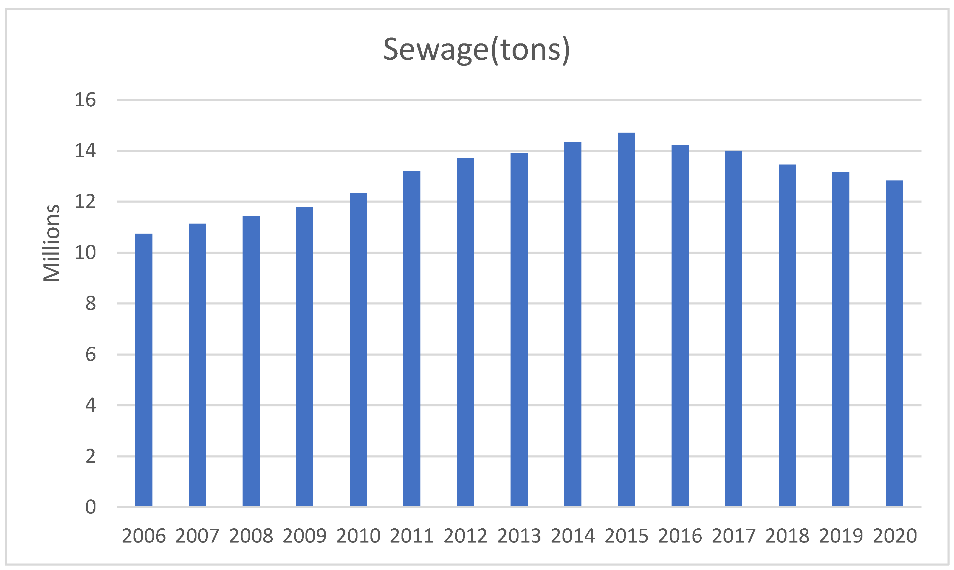
| Capital: Capital stock (CNY 10,000) | Sewage discharge of industrial and domestic waste water by region (10 000 tons): Undesired output |
| Water consumption: Water use (100 million cu. m) |
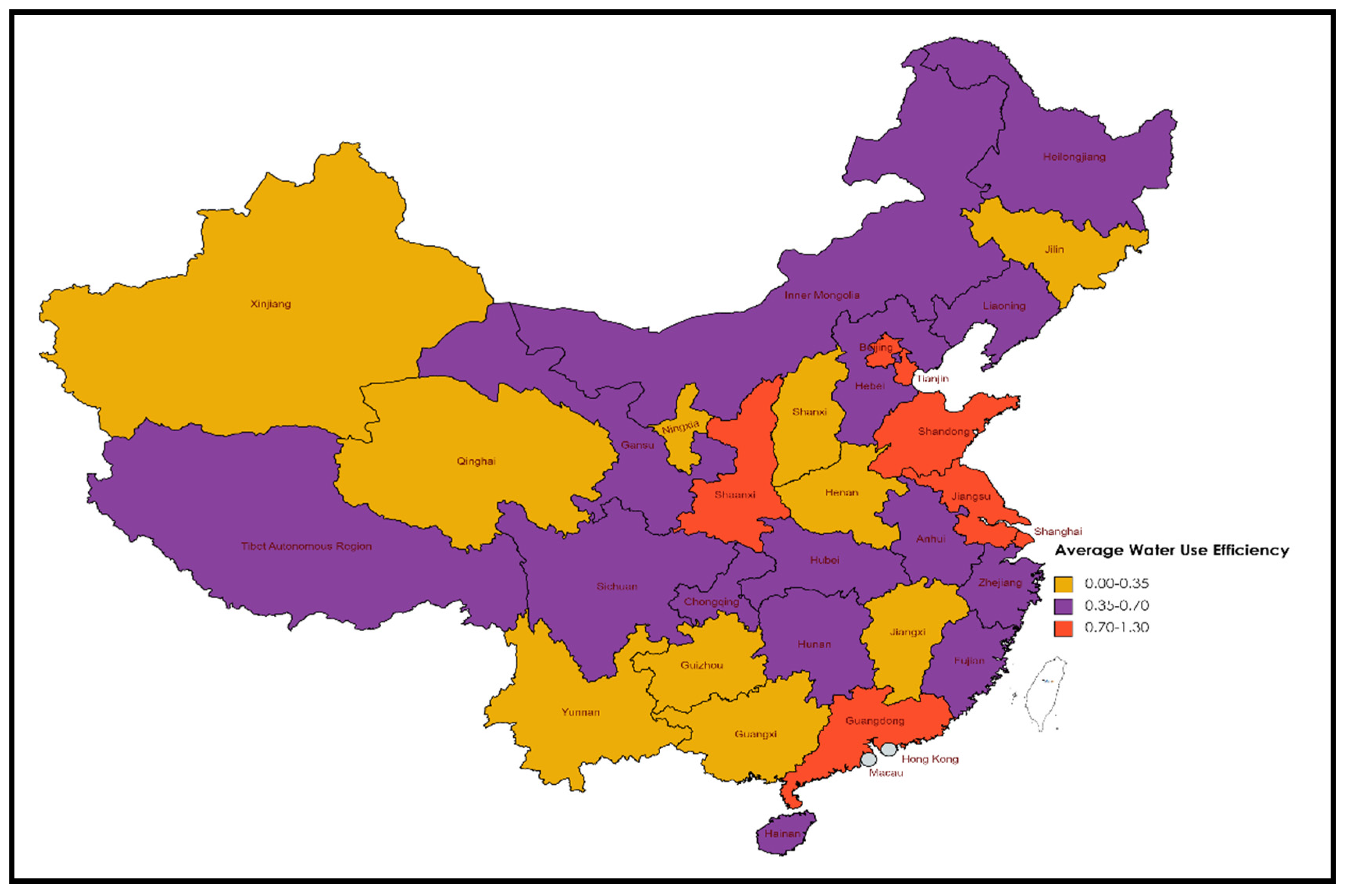
| Year | WUE |
|---|---|
| 2006 | 0.6100 |
| 2007 | 0.5981 |
| 2008 | 0.5902 |
| 2009 | 0.5597 |
| 2010 2011 | 0.5822 0.5321 |
| Avg. 2006–2011 | 0.5787 |
| 2012 | 0.5379 |
| 2013 | 0.5373 |
| 2014 | 0.5292 |
| 2015 | 0.538 |
| 2016 | 0.5186 |
| 2017 | 0.5155 |
| 2018 | 0.4192 |
| 2019 | 0.3647 |
| 2020 | 0.3885 |
| Avg. 2012–2020 | 0.4832 |
| Avg. 2006–2020 | 0.5214 |
| Province | GWE | MWE | TGR | |||
|---|---|---|---|---|---|---|
| Mean | S.D | Mean | S.D | Mean | S.D | |
| Anhui | 0.908 | 0.1744 | 0.377 | 0.0411 | 0.435 | 0.1228 |
| Beijing | 1.083 | 0.2551 | 1.083 | 0.2551 | 1 | 0 |
| Fujian | 0.44 | 0.046 | 0.44 | 0.046 | 1 | 0 |
| Gansu | 0.911 | 0.1604 | 0.41 | 0.0723 | 0.463 | 0.1091 |
| Guangdong | 0.904 | 0.1825 | 0.837 | 0.1985 | 0.933 | 0.1436 |
| Guangxi | 0.742 | 0.2268 | 0.356 | 0.0437 | 0.518 | 0.1473 |
| Guizhou | 0.718 | 0.201 | 0.337 | 0.0676 | 0.495 | 0.1258 |
| Hainan | 0.358 | 0.0395 | 0.358 | 0.0395 | 1 | 0 |
| Hebei | 0.619 | 0.176 | 0.616 | 0.1673 | 0.998 | 0.0097 |
| Henan | 0.649 | 0.0284 | 0.322 | 0.0513 | 0.497 | 0.0795 |
| Heilongjiang | 0.962 | 0.2499 | 0.5 | 0.2509 | 0.503 | 0.1528 |
| Hubei | 0.966 | 0.1642 | 0.399 | 0.0418 | 0.428 | 0.1006 |
| Hunan | 1.151 | 0.107 | 0.446 | 0.0447 | 0.393 | 0.0651 |
| Jilin | 0.884 | 0.2746 | 0.329 | 0.0784 | 0.39 | 0.0855 |
| Jiangsu | 0.7 | 0.1022 | 0.7 | 0.1022 | 1 | 0 |
| Jiangxi | 0.793 | 0.2032 | 0.346 | 0.0364 | 0.462 | 0.1259 |
| Liaoning | 0.432 | 0.0928 | 0.432 | 0.0928 | 1 | 0 |
| Inner Mongolia | 1.184 | 0.0776 | 0.644 | 0.2787 | 0.534 | 0.2078 |
| Ningxia | 0.413 | 0.0324 | 0.223 | 0.0375 | 0.542 | 0.0901 |
| Qinghai | 0.389 | 0.0659 | 0.216 | 0.0612 | 0.55 | 0.1139 |
| Shandong | 0.736 | 0.2141 | 0.735 | 0.2135 | 1 | 0.0012 |
| Shanxi | 0.721 | 0.1662 | 0.348 | 0.0702 | 0.49 | 0.0829 |
| Shaanxi | 1.49 | 0.045 | 1.02 | 0.1311 | 0.685 | 0.087 |
| Shanghai | 1.238 | 0.1853 | 1.236 | 0.1854 | 0.999 | 0.0055 |
| Sichuan | 1.015 | 0.0688 | 0.397 | 0.0401 | 0.393 | 0.0486 |
| Tianjin | 1.025 | 0.3383 | 1.012 | 0.331 | 0.99 | 0.0111 |
| Tibet | 0.944 | 0.2812 | 0.43 | 0.3236 | 0.509 | 0.349 |
| Xinjiang | 0.651 | 0.2091 | 0.302 | 0.064 | 0.483 | 0.1037 |
| Yunnan | 0.601 | 0.2029 | 0.346 | 0.0916 | 0.591 | 0.0935 |
| Zhejiang | 0.558 | 0.082 | 0.558 | 0.082 | 1 | 0 |
| Chongqing | 0.973 | 0.1878 | 0.408 | 0.0766 | 0.426 | 0.0638 |
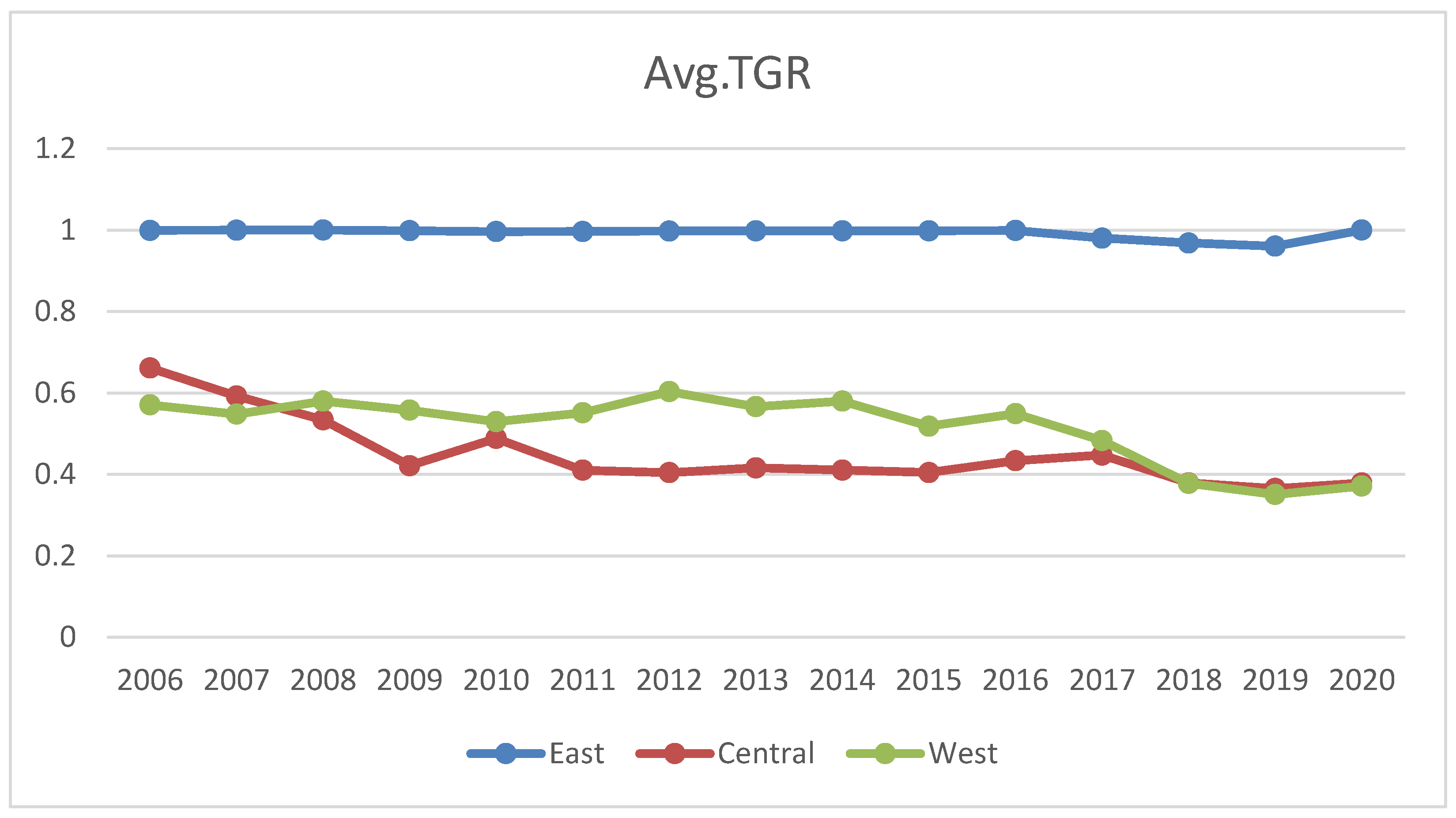
| Region | Province | MLI | EC | TC. |
|---|---|---|---|---|
| Central | Anhui | 1.1097 | 0.9899 | 1.125 |
| Central | Henan | 1.079 | 0.9656 | 1.1212 |
| Central | Heilongjiang | 1.0768 | 0.9096 | 1.1938 |
| Central | Hubei | 1.1235 | 0.9886 | 1.1396 |
| Central | Hunan | 1.1153 | 0.9843 | 1.1404 |
| Central | Jilin | 1.1096 | 0.9758 | 1.1324 |
| Central | Jiangxi | 1.0792 | 0.9895 | 1.0951 |
| Central | Shanxi | 1.0944 | 0.9759 | 1.1255 |
| Ave. Central | 1.0984 | 0.9724 | 1.1341 | |
| East | Beijing | 1.1214 | 1.0573 | 1.1527 |
| East | Fujian | 1.1317 | 0.996 | 1.1438 |
| East | Guangdong | 1.0996 | 0.9548 | 1.1554 |
| East | Hainan | 1.1045 | 0.9825 | 1.1364 |
| East | Hebei | 1.1633 | 0.9879 | 1.1812 |
| East | Jiangsu | 1.1927 | 1.0012 | 1.2098 |
| East | Liaoning | 1.0793 | 0.9753 | 1.116 |
| East | Shandong | 1.111 | 0.937 | 1.2029 |
| East | Shanghai | 1.1063 | 1.0223 | 1.084 |
| East | Tianjin | 1.0715 | 0.9409 | 1.1734 |
| East | Zhejiang | 1.1313 | 0.9724 | 1.1689 |
| Ave. East | 1.1193 | 0.9843 | 1.1568 | |
| West | Gansu | 1.1218 | 0.9689 | 1.1683 |
| West | Guangxi | 1.1167 | 0.9909 | 1.1255 |
| West | Guizhou | 1.1501 | 0.9891 | 1.1654 |
| West | Inner Mongolia | 1.1725 | 0.921 | 1.2896 |
| West | Ningxia | 1.0947 | 0.9934 | 1.094 |
| West | Qinghai | 1.0782 | 0.9935 | 1.091 |
| West | Shaanxi | 1.2182 | 1.0206 | 1.2287 |
| West | Sichuan | 1.1155 | 0.9927 | 1.1302 |
| West | Tibet | 1.359 | 0.9064 | 1.5836 |
| West | Xinjiang | 1.0806 | 0.962 | 1.1245 |
| West | Yunnan | 1.1464 | 0.9787 | 1.1823 |
| West | Chongqing | 1.1439 | 1.0182 | 1.1384 |
| Ave. West | 1.1498 | 0.9779 | 1.1935 |
| Hypothesis Test Summary | ||||
|---|---|---|---|---|
| Null Hypothesis | Test | Sig. | Decision | |
| 1 | The distribution of Avg. WUE is identical for both time periods. | Independent-Samples Mann–Whitney U Test | 0.003 a | Reject the null hypothesis. |
| 2 | The distribution of Avg. MLI is identical for both time periods. | Independent-Samples Mann–Whitney U Test | 0.066 a | Retain the null hypothesis. |
| 3 | The distribution of Avg. TC is identical for both time periods. | Independent-Samples Mann–Whitney U Test | 0.234 a | Retain the null hypothesis |
| 4 | The distribution of Avg. EC is identical for both time periods. | Independent-Samples Mann–Whitney U Test | 0.278 a | Retain the null hypothesis |
| Hypothesis Test Summary | ||||
|---|---|---|---|---|
| Null Hypothesis | Test | Sig. | Decision | |
| 1 | The distribution of Avg. WUE is identical across China’s three distinct regions. | Independent-Samples Kruskal–Wallis Test | 0.002 | Reject the null hypothesis. |
| 2 | The distribution of Avg. MI change is identical across China’s three distinct regions. | Independent-Samples Kruskal–Wallis Test | 0.000 | Reject the null hypothesis |
| 3 | The distribution of Avg. Technology is identical across China’s three distinct regions. | Independent-Samples Kruskal–Wallis Test | 0.007 | Reject the null hypothesis |
| 4 | The distribution of Avg. Efficiency change is identical across China’s three distinct regions. | Independent-Samples Kruskal–Wallis Test | 0.350 | Retain the null hypothesis |
Publisher’s Note: MDPI stays neutral with regard to jurisdictional claims in published maps and institutional affiliations. |
© 2022 by the authors. Licensee MDPI, Basel, Switzerland. This article is an open access article distributed under the terms and conditions of the Creative Commons Attribution (CC BY) license (https://creativecommons.org/licenses/by/4.0/).
Share and Cite
Shah, W.U.H.; Lu, Y.; Hao, G.; Yan, H.; Yasmeen, R. Impact of “Three Red Lines” Water Policy (2011) on Water Usage Efficiency, Production Technology Heterogeneity, and Determinant of Water Productivity Change in China. Int. J. Environ. Res. Public Health 2022, 19, 16459. https://doi.org/10.3390/ijerph192416459
Shah WUH, Lu Y, Hao G, Yan H, Yasmeen R. Impact of “Three Red Lines” Water Policy (2011) on Water Usage Efficiency, Production Technology Heterogeneity, and Determinant of Water Productivity Change in China. International Journal of Environmental Research and Public Health. 2022; 19(24):16459. https://doi.org/10.3390/ijerph192416459
Chicago/Turabian StyleShah, Wasi Ul Hassan, Yuting Lu, Gang Hao, Hong Yan, and Rizwana Yasmeen. 2022. "Impact of “Three Red Lines” Water Policy (2011) on Water Usage Efficiency, Production Technology Heterogeneity, and Determinant of Water Productivity Change in China" International Journal of Environmental Research and Public Health 19, no. 24: 16459. https://doi.org/10.3390/ijerph192416459
APA StyleShah, W. U. H., Lu, Y., Hao, G., Yan, H., & Yasmeen, R. (2022). Impact of “Three Red Lines” Water Policy (2011) on Water Usage Efficiency, Production Technology Heterogeneity, and Determinant of Water Productivity Change in China. International Journal of Environmental Research and Public Health, 19(24), 16459. https://doi.org/10.3390/ijerph192416459