New Fixed Assets Investment Project Environmental Performance and Influencing Factors—An Empirical Analysis in China’s Optics Valley

Abstract
1. Introduction
2. Literature Review
2.1. Environmental Performance Definition
2.2. Environmental Performance Evaluation
2.3. Factors Affecting Environmental Performance
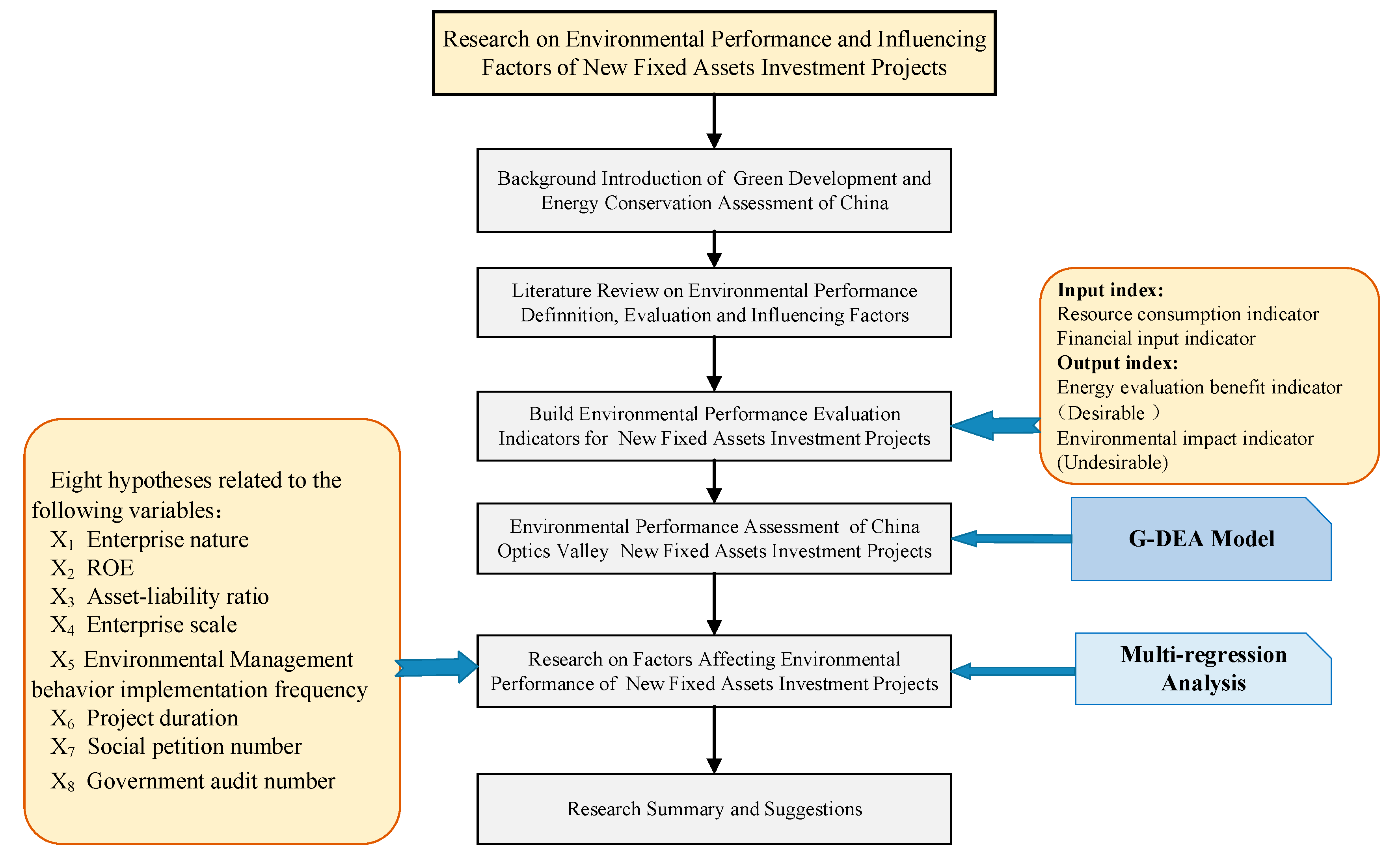
3. New Fixed Assets Investment Project Environmental Performance Measurements
3.1. Generalized DEA Model with Undesirable Output
3.2. Model Construction and Validity Judgment
3.3. Screening of Environmental Performance Evaluation Indicators for New Fixed Assets Investment Projects
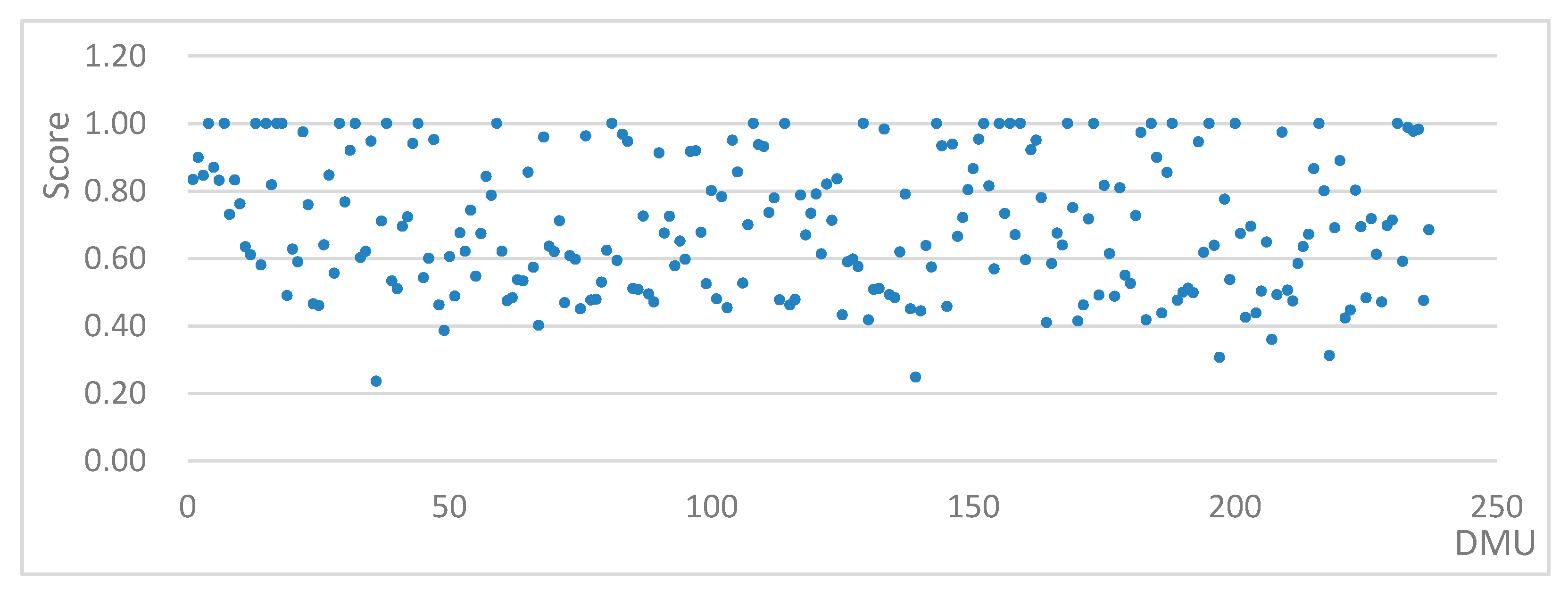
3.4. Environmental Performance Assessment Process and Results Analysis
4. Factors Affecting the Environmental Performance of New Fixed Assets Investment Projects
4.1. Research Hypothesis
4.2. Variable Design
- (1)
- The nature of the enterprise (Is it a listed company? Yes = 1; no = 0);
- (2)
- Corporate profitability (return on net assets, indicating the ability of the net assets to generate profits);
- (3)
- Financial status (the asset-liability ratio is an effective indicator for evaluating the financial health of enterprises, and is also an indicator that can measure the ability of enterprises to use creditor funds for reasonable business activities);
- (4)
- Enterprise scale (registered capital of the enterprise, <10 million CNY = 1, 10–50 million CNY = 2, 50–100 million CNY = 3, 100–500 million CNY = 4, 500 million–1 billion CNY = 5, >1 billion CNY = 6);
- (5)
- Implementation frequency of environmental management behavior (based on the relevant national environmental policies, regulations, and standards (Table 3);
- (6)
- Construction period (the time span from the start of construction to the completion of the project, by month).
- (7)
- The number of letters and visits from social groups;
- (8)
- The number of supervisory actions taken by the government.
4.3. Data Sources
4.4. Model Selection and Result Analysis
4.4.1. Descriptive Statistical Analysis
4.4.2. Statistical Tests and Regression Analyses
4.4.3. Discussion
5. Conclutions
Author Contributions
Funding
Conflicts of Interest
References
- Chevallier, J.; Goutte, S. Estimation of Lévy-driven Ornstein–Uhlenbeck processes: Application to modeling of CO2 and fuel-switching. Ann. Oper. Res. 2017, 255, 169–197. [Google Scholar] [CrossRef]
- Cai, Y.; Lu, Y.; Stegman, A.; Newth, D. Simulating emissions intensity targets with energy economic models: Algorithm and application. Ann. Oper. Res. 2017, 255, 141–155. [Google Scholar] [CrossRef]
- Mikko, P.; Pasi, P.; Marko, T.; Jouni, T. Perspectives to Performance of Environment and Health Assessments and Modelsâ—From Outputs to Outcomes? Int. J. Environ. Res. Public Health 2013, 10, 2621–2642. [Google Scholar]
- Suasana, I.G.A.K.G.; Ekawati, N.W. Environmental commitment and green innovation reaching success new products of creative industry in Bali. J. Bus. Retail Manag. Res. 2018, 12. [Google Scholar] [CrossRef]
- Zehir, C.; Balak, D. Market Dynamism and Firm Performance Relation: The Mediating Effects of Positive Environment Conditions and Firm Innovativeness. EMAJ Emerg. Mark. J. 2018, 8, 45–51. [Google Scholar] [CrossRef]
- Dües, C.M.; Tan, K.H.; Lim, M. Green as the new Lean: How to use Lean practices as a catalyst to greening your supply chain. J. Clean. Prod. 2013, 40, 93–100. [Google Scholar] [CrossRef]
- Qiu, Y.; Shaukat, A.; Tharyan, R. Environmental and social disclosures: Link with corporate financial performance. Br. Account. Rev. 2016, 48, 102–116. [Google Scholar] [CrossRef]
- Braam, G.J.; de Weerd, L.U.; Hauck, M.; Huijbregts, M.A. Determinants of corporate environmental reporting: The importance of environmental performance and assurance. J. Clean. Prod. 2016, 129, 724–734. [Google Scholar] [CrossRef]
- Chuang, S.-P.; Huang, S.-J. The effect of environmental corporate social responsibility on environmental performance and business competitiveness: The mediation of green information technology capital. J. Bus. Ethics 2018, 150, 991–1009. [Google Scholar] [CrossRef]
- Latan, H.; Jabbour, C.J.C.; de Sousa Jabbour, A.B.L.; Wamba, S.F.; Shahbaz, M. Effects of environmental strategy, environmental uncertainty and top management’s commitment on corporate environmental performance: The role of environmental management accounting. J. Clean. Prod. 2018, 180, 297–306. [Google Scholar] [CrossRef]
- Brooks, C.; Oikonomou, I. The effects of environmental, social and governance disclosures and performance on firm value: A review of the literature in accounting and finance. Br. Account. Rev. 2018, 50, 1–15. [Google Scholar] [CrossRef]
- Koskela, M.; Vehmas, J. Defining eco-efficiency: A case study on the Finnish forest industry. Bus. Strategy Environ. 2012, 21, 546–566. [Google Scholar] [CrossRef]
- Ruf, B.M.; Muralidhar, K.; Brown, R.M.; Janney, J.J.; Paul, K. An empirical investigation of the relationship between change in corporate social performance and financial performance: A stakeholder theory perspective. J. Bus. Ethics 2001, 32, 143–156. [Google Scholar] [CrossRef]
- Carroll, A.B. A commentary and an overview of key questions on corporate social performance measurement. Bus. Soc. 2000, 39, 466–478. [Google Scholar] [CrossRef]
- Lankoski, L. Determinants of Environmental Profit: An Analysis of the Firm-Level Relationship between Environmental Performance and Economic Performance; Helsinki University of Technology: Espoo, Finland, 2000. [Google Scholar]
- Wood, D.J. Measuring corporate social performance: A review. Int. J. Manag. Rev. 2010, 12, 50–84. [Google Scholar] [CrossRef]
- Wang, J.; Wang, R.; Zhu, Y.; Li, J. Life cycle assessment and environmental cost accounting of coal-fired power generation in China. Energy Policy 2018, 115, 374–384. [Google Scholar] [CrossRef]
- Wang, Q.; Yang, Z. Industrial water pollution, water environment treatment, and health risks in China. Environ. Pollut. 2016, 218, 358–365. [Google Scholar] [CrossRef]
- Wang, Z.; Yang, L. Delinking indicators on regional industry development and carbon emissions: Beijing–Tianjin–Hebei economic band case. Ecol. Indic. 2015, 48, 41–48. [Google Scholar] [CrossRef]
- Ye, F.F.; Yang, L.H.; Wang, Y.M. An interval efficiency evaluation model for air pollution management based on indicators integration and different perspectives. J. Clean. Prod. 2019, 118945. [Google Scholar] [CrossRef]
- Solarin, S.A.; Al-Mulali, U.; Musah, I.; Ozturk, I. Investigating the pollution haven hypothesis in Ghana: An empirical investigation. Energy 2017, 124, 706–719. [Google Scholar] [CrossRef]
- Song, M.-L.; Fisher, R.; Wang, J.-L.; Cui, L.-B. Environmental performance evaluation with big data: Theories and methods. Ann. Oper. Res. 2018, 270, 459–472. [Google Scholar] [CrossRef]
- Qu, S.; Zhou, Y.; Zhang, Y.; Wahab, M.; Zhang, G.; Ye, Y. Optimal strategy for a green supply chain considering shipping policy and default risk. Comput. Ind. Eng. 2019, 131, 172–186. [Google Scholar] [CrossRef]
- Huang, R.; Qu, S.; Yang, X.; Liu, Z. Multi-stage distributionally robust optimization with risk aversion. J. Ind. Manag. Optim. 2019, 13. [Google Scholar] [CrossRef]
- Freedman, M.; Patten, D.M. Evidence on the pernicious effect of financial report environmental disclosure. Account. Forum (Taylor Fr.) 2004, 28, 27–41. [Google Scholar]
- Hamilton, J.T. Pollution as news: Media and stock market reactions to the toxics release inventory data. J. Environ. Econ. Manag. 1995, 28, 98–113. [Google Scholar] [CrossRef]
- Arabi, B.; Doraisamy, S.M.; Emrouznejad, A.; Khoshroo, A. Eco-efficiency measurement and material balance principle: An application in power plants Malmquist Luenberger Index. Ann. Oper. Res. 2017, 255, 221–239. [Google Scholar] [CrossRef]
- Tyteca, D. On the Measurement of the Environmental Performance of Firms—A Literature Review and a Productive Efficiency Perspective. J. Environ. Manag. 1996, 46, 281–308. [Google Scholar] [CrossRef]
- Charnes, A.; Cooper, W.W.; Rhodes, E. Measuring the efficiency of decision making units. Eur. J. Oper. Res. 1978, 2, 429–444. [Google Scholar] [CrossRef]
- Ramanathan, R.; Ramanathan, U.; Bentley, Y. The debate on flexibility of environmental regulations, innovation capabilities and financial performance—A novel use of DEA. Omega 2018, 75, 131–138. [Google Scholar] [CrossRef]
- Park, Y.S.; Lim, S.H.; Egilmez, G.; Szmerekovsky, J. Environmental efficiency assessment of US transport sector: A slack-based data envelopment analysis approach. Transp. Res. Part D Transp. Environ. 2018, 61, 152–164. [Google Scholar] [CrossRef]
- Sueyoshi, T.; Goto, M.; Ueno, T. Performance analysis of US coal-fired power plants by measuring three DEA efficiencies. Energy Policy 2010, 38, 1675–1688. [Google Scholar] [CrossRef]
- Hu, Q. Research on Correlation between Environmental Performance and Financial Performance of Listed Companies. China’s Popul. Resour. Environ. 2012, 6, 25–34. [Google Scholar]
- Zhou, H.; Li, Z. Environmental Management System Certification Improves Environmental Management Performance. Environ. Sustain. Dev. 2013, 2, 102–105. [Google Scholar]
- Lin, W.L.; Ho, J.A.; Sambasivan, M. Impact of Corporate Political Activity on the Relationship Between Corporate Social Responsibility and Financial Performance: A Dynamic Panel Data Approach. Sustainability 2018, 11, 60. [Google Scholar] [CrossRef]
- Yin, H.; Ma, C. International integration: A hope for a greener China? Int. Mark. Rev. 2009, 26, 348–367. [Google Scholar] [CrossRef]
- Dawkins, C.E.; Fraas, J.W. Erratum to: Beyond acclamations and excuses: Environmental performance, voluntary environmental disclosure and the role of visibility. J. Bus. Ethics 2011, 99, 383–397. [Google Scholar] [CrossRef]
- Xiao, C.; Wang, Q.; van der Vaart, T.; van Donk, D.P. When does corporate sustainability performance pay off? The impact of country-level sustainability performance. Ecol. Econ. 2018, 146, 325–333. [Google Scholar] [CrossRef]
- Pineiro-Chousa, J.; Romero-Castro, N.; Vizcaíno-González, M. Inclusions in and Exclusions from the S&P 500 Environmental and Socially Responsible Index: A Fuzzy-Set Qualitative Comparative Analysis. Sustainability 2019, 11, 1211. [Google Scholar]
- Farooq, O.; Farooq, M.; Reynaud, E. Does Employees’ Participation in Decision Making Increase the level of Corporate Social and Environmental Sustainability? An Investigation in South Asia. Sustainability 2019, 11, 511. [Google Scholar] [CrossRef]
- Chen, Y.; Yang, Y.; Du, D. Research on Performance Evaluation of Provincial Ecological Environment Based on Cloud Model. Soft Sci. 2018, 1, 100–103. [Google Scholar]
- Long, J.; Pan, J.; Feng, T. Research on the Influence of Lean Production and Enterprise Environmental Management on the Sustainable Development Performance of Manufacturing Industry. Soft Sci. 2018, 4, 68–71. [Google Scholar]
- Haihua, Z.; Shuanglong, W. Community environmental pressure, environmental information communication and environmental performance. Soft Sci. 2018, 32, 80–83. [Google Scholar]
- Jin, Y.; Zheng, S.; Tang, D.; Feng, Q. Environmental Performance Evaluation of New Fixed Assets Investment Projects—Taking Wuhan East Lake High-Tech Development Zone as an Example. In International Conference on Management Science and Engineering Management; Springer: Cham, Switzerland, 2018; pp. 1327–1340. [Google Scholar]
- Petrash, J.M.; Cooper III, W.S.; Baskerville, S.L.; Blanton, M.S. Report of the Legislation and Regulatory Reform Committee. Energy Law J. 2007, 28, 375. [Google Scholar]
- James, P. Business environmental performance measurement. Bus. Strategy Environ. 1994, 3, 59–67. [Google Scholar] [CrossRef]
- Zheng, S.; Jin, Y.; Zhang, J. Investigation and Study on the Influencing Factors of Enterprise Environmental Management Behavior under the Background of Two-oriented Society—Taking Wuhan East Lake High-tech Development Zone (China’s Optical Valley) as an Example. Sci. Technol. Prog. Policy 2015, 11, 83–88. [Google Scholar]
- Du, X.; Weng, J.; Zeng, Q.; Chang, Y.; Pei, H. Do Lenders Applaud Corporate Environmental Performance? Evidence from Chinese Private-Owned Firms. J. Bus. Ethics 2017, 143, 179–207. [Google Scholar] [CrossRef]


| Target Layer | Input/Output Indicator | Specific Indicators | ||
|---|---|---|---|---|
| Environmental impact indicators | Input index | Resource consumption indicators | Power consumption | |
| Water Consumption | ||||
| Steam consumption | ||||
| Natural gas consumption | ||||
| Financial input indicator | Total investment | |||
| Output index | Desirable output | Energy evaluation benefit indicator | Energy saving quantity | |
| Undesirable output | Environmental impact indicators | Carbon dioxide emissions | ||
| Sulfur dioxide emissions | ||||
| DMU | Score | DMU | Score | DMU | Score | DMU | Score | DMU | Score | DMU | Score |
|---|---|---|---|---|---|---|---|---|---|---|---|
| 1 | 0.83403 | 41 | 0.69529 | 81 | 1 | 121 | 0.61373 | 161 | 0.92160 | 201 | 0.67344 |
| 2 | 0.89979 | 42 | 0.72310 | 82 | 0.59394 | 122 | 0.82040 | 162 | 0.95035 | 202 | 0.42593 |
| 3 | 0.84619 | 43 | 0.94080 | 83 | 0.96806 | 123 | 0.71306 | 163 | 0.78017 | 203 | 0.69537 |
| 4 | 1 | 44 | 1 | 84 | 0.94723 | 124 | 0.83562 | 164 | 0.41045 | 204 | 0.43802 |
| 5 | 0.87032 | 45 | 0.54297 | 85 | 0.51122 | 125 | 0.43246 | 165 | 0.58532 | 205 | 0.50311 |
| 6 | 0.83144 | 46 | 0.60018 | 86 | 0.50787 | 126 | 0.58977 | 166 | 0.67552 | 206 | 0.64870 |
| 7 | 1 | 47 | 0.95178 | 87 | 0.72552 | 127 | 0.59848 | 167 | 0.63967 | 207 | 0.35988 |
| 8 | 0.73059 | 48 | 0.46232 | 88 | 0.49472 | 128 | 0.57591 | 168 | 1 | 208 | 0.49269 |
| 9 | 0.83246 | 49 | 0.38664 | 89 | 0.47128 | 129 | 1 | 169 | 0.75094 | 209 | 0.97435 |
| 10 | 0.76183 | 50 | 0.60499 | 90 | 0.91254 | 130 | 0.41780 | 170 | 0.41471 | 210 | 0.50609 |
| 11 | 0.63478 | 51 | 0.48843 | 91 | 0.67503 | 131 | 0.50822 | 171 | 0.46198 | 211 | 0.47409 |
| 12 | 0.61079 | 52 | 0.67561 | 92 | 0.72500 | 132 | 0.51113 | 172 | 0.71713 | 212 | 0.58472 |
| 13 | 1 | 53 | 0.62132 | 93 | 0.57777 | 133 | 0.98343 | 173 | 1 | 213 | 0.63503 |
| 14 | 0.58068 | 54 | 0.74319 | 94 | 0.65162 | 134 | 0.49273 | 174 | 0.49167 | 214 | 0.67161 |
| 15 | 1 | 55 | 0.54714 | 95 | 0.59773 | 135 | 0.48347 | 175 | 0.81647 | 215 | 0.86567 |
| 16 | 0.81828 | 56 | 0.67385 | 96 | 0.91689 | 136 | 0.61918 | 176 | 0.61432 | 216 | 1 |
| 17 | 1.00000 | 57 | 0.84309 | 97 | 0.91936 | 137 | 0.79036 | 177 | 0.48824 | 217 | 0.80032 |
| 18 | 1 | 58 | 0.78713 | 98 | 0.67761 | 138 | 0.45114 | 178 | 0.80943 | 218 | 0.31238 |
| 19 | 0.48971 | 59 | 1 | 99 | 0.52481 | 139 | 0.24850 | 179 | 0.55034 | 219 | 0.69154 |
| 20 | 0.62746 | 60 | 0.62164 | 100 | 0.80127 | 140 | 0.44438 | 180 | 0.52532 | 220 | 0.88936 |
| 21 | 0.59018 | 61 | 0.47440 | 101 | 0.48057 | 141 | 0.63795 | 181 | 0.72654 | 221 | 0.42359 |
| 22 | 0.97459 | 62 | 0.48341 | 102 | 0.78251 | 142 | 0.57442 | 182 | 0.97385 | 222 | 0.44712 |
| 23 | 0.75880 | 63 | 0.53685 | 103 | 0.45369 | 143 | 1 | 183 | 0.41826 | 223 | 0.80231 |
| 24 | 0.46537 | 64 | 0.53311 | 104 | 0.95014 | 144 | 0.93345 | 184 | 1 | 224 | 0.69384 |
| 25 | 0.46057 | 65 | 0.85563 | 105 | 0.85613 | 145 | 0.45773 | 185 | 0.89982 | 225 | 0.48331 |
| 26 | 0.64031 | 66 | 0.57385 | 106 | 0.52725 | 146 | 0.93844 | 186 | 0.43862 | 226 | 0.71790 |
| 27 | 0.84698 | 67 | 0.40228 | 107 | 0.69964 | 147 | 0.66554 | 187 | 0.85442 | 227 | 0.61203 |
| 28 | 0.55617 | 68 | 0.95948 | 108 | 1 | 148 | 0.72128 | 188 | 1 | 228 | 0.47119 |
| 29 | 1 | 69 | 0.63619 | 109 | 0.93713 | 149 | 0.80350 | 189 | 0.47609 | 229 | 0.69730 |
| 30 | 0.76708 | 70 | 0.61983 | 110 | 0.93170 | 150 | 0.86606 | 190 | 0.49977 | 230 | 0.71354 |
| 31 | 0.92010 | 71 | 0.71120 | 111 | 0.73578 | 151 | 0.95307 | 191 | 0.51154 | 231 | 1 |
| 32 | 1 | 72 | 0.46924 | 112 | 0.77910 | 152 | 1 | 192 | 0.49861 | 232 | 0.59157 |
| 33 | 0.60245 | 73 | 0.60836 | 113 | 0.47749 | 153 | 0.81464 | 193 | 0.94534 | 233 | 0.98787 |
| 34 | 0.62087 | 74 | 0.59793 | 114 | 1 | 154 | 0.56920 | 194 | 0.61785 | 234 | 0.97681 |
| 35 | 0.94771 | 75 | 0.45065 | 115 | 0.46239 | 155 | 1 | 195 | 1 | 235 | 0.98257 |
| 36 | 0.23667 | 76 | 0.96320 | 116 | 0.47798 | 156 | 0.73294 | 196 | 0.63867 | 236 | 0.47521 |
| 37 | 0.71091 | 77 | 0.47641 | 117 | 0.78758 | 157 | 1 | 197 | 0.30682 | 237 | 0.68523 |
| 38 | 1 | 78 | 0.47882 | 118 | 0.66981 | 158 | 0.67038 | 198 | 0.77594 | ||
| 39 | 0.53313 | 79 | 0.53002 | 119 | 0.73356 | 159 | 1 | 199 | 0.53735 | ||
| 40 | 0.51001 | 80 | 0.62453 | 120 | 0.79115 | 160 | 0.59592 | 200 | 1 |
| No. | Environmental Management Examples | Relevant Legal Basis |
|---|---|---|
| 1 | The enterprise regularly conducts environmental training for employees | Environmental protection law of the People’s Republic of China; Environmental impact assessment law of the People’s Republic of China; Law of the People’s Republic of China on energy conservation; Regulations on the administration of environmental protection for construction projects. |
| 2 | Pollutant emissions enterprise system monitoring indicators | |
| 3 | The enterprise regularly publishes environmental reports | |
| 4 | The enterprise has implemented an environmental plan | |
| 5 | The enterprise has clear environmental requirements for the raw materials and suppliers. | |
| 6 | Extensive publicity and education on environmental protection and energy saving | |
| 7 | The enterprise’s products have an ISO9001 quality management system certification. | |
| 8 | The enterprise’s products have an ISO14001 environmental management system certification. | |
| 9 | The enterprise has a dedicated department or dedicated staff responsible for environmental management | |
| 10 | The enterprise has established an environmental management system with the supplier | |
| 11 | The enterprise purchases environmentally friendly equipment | |
| 12 | The enterprise evaluates environmental performance based on policy objectives and seeks reasonable improvements | |
| 13 | The enterprise has a clean production audit | |
| 14 | The enterprise has a documented environmental policy to guide environmental management | |
| 15 | The enterprise’s products have obtained GB/T18001 occupational health and safety management system certification |
| Variable Type | Variable | Variable Indicator Selection | Abbeviation |
|---|---|---|---|
| Dependent variable | Environmental performance | (0, 1] | Y |
| Independent variable | Enterprise nature | Listing = 1, no listing = 0 | X1 |
| ROE | Roe = net profit/net assets | X2 | |
| Asset-liability ratio | Asset-liability ratio = total liabilities/total assets | X3 | |
| Enterprise scale | Registered capital | X4 | |
| Environmental Management behavior implementation frequency | IFEMB, the data comes from questionnaire statistics | X5 | |
| Project duration | The length of months from the start of construction to completion | X6 | |
| Social petition number | Number of complaints and letters from residents of surrounding communities | X7 | |
| Government audit number | Number of times the enterprise was audited by the environment during the project construction period | X8 |
| Variable | N | Minimum Value | Maximum | Mean | Standard Deviation |
|---|---|---|---|---|---|
| Y Environmental performance | 237 | 0.23667 | 1.000 | 0.69759 | 0.198500 |
| X1 Enterprise nature | 237 | 0 | 1 | 0.03 | 0.170 |
| X2 ROE | 237 | −1.25 | 2.68 | 0.1598 | 0.36811 |
| X3 Asset-liability ratio | 237 | 0.011 | 1.211 | 0.48746 | 0.255657 |
| X4 Enterprise scale | 237 | 1 | 6 | 3.18 | 1.336 |
| X5 Environmental management behavior implementation frequency | 237 | 3 | 37 | 19.36 | 7.556 |
| X6 Project duration | 237 | 2 | 83 | 28.05 | 13.240 |
| X7 Social petition number | 237 | 0 | 8 | 2.56 | 1.842 |
| X8 Government audit number | 237 | 1 | 5 | 3.31 | 1.117 |
| Valid N (list state) | 237 |
| Y | X1 | X2 | X3 | X4 | X5 | X6 | X7 | X8 | |
|---|---|---|---|---|---|---|---|---|---|
| Y | 1 | ||||||||
| X1 | 0.127 * | 1 | |||||||
| X2 | 0.119 * | −0.041 | 1 | ||||||
| X3 | −0.129 * | −0.050 | 0.052 | 1 | |||||
| X4 | −0.019 * | −0.062 | 0.015 | 0.047 | 1 | ||||
| X5 | 0.175 ** | 0.127 | −0.107 | −0.033 | −0.141 ** | 1 | |||
| X6 | −0.088 ** | −0.103 | −0.023 | −0.031 | 0.459 ** | −0.182 ** | 1 | ||
| X7 | −0.216 ** | −0.067 | 0.102 | 0.036 | 0.112 ** | −0.047 ** | 0.169 ** | 1 | |
| X8 | 0.155 ** | 0.019 | −0.155 | −0.049 | −0.054 * | 0.295 ** | −0.148 | −0.315 ** | 1 |
| Model | R | R Square | Adjust R Square | Standard Estimated Error |
|---|---|---|---|---|
| 1 | 0.633 a | 0.401 | 0.349 | 5.85059 |
| Model | Sum of Square | Df | Mean Square | F | Sig. | |
|---|---|---|---|---|---|---|
| 1 | Regression | 8.073 | 8 | 1.009 | 187.677 | 0.000 a |
| Residual | 1.226 | 228 | 0.005 | |||
| Total | 9.299 | 236 | ||||
| MODEL | Non-Standardized Coefficient | Standard Coefficient | t | Sig. | Collinear Statistic | ||
|---|---|---|---|---|---|---|---|
| B | Standard error | trial version | Tolerance | VIF | |||
| (constant) | 0.392 | 0.037 | 10.512 | 0.000 | |||
| X1 Enterprise nature | 0.126 | 0.029 | 0.122 | 2.899 | 0.027 | 0.953 | 1.050 |
| X2 ROE | 0.101 | 0.021 | 0.133 | 3.625 | 0.032 | 0.969 | 1.032 |
| X3 Asset-liability ratio | −0.010 | 0.019 | −0.012 | −2.015 | 0.007 | 0.988 | 1.012 |
| X4 Enterprise scale | −0.005 | 0.004 | −0.034 | −1.148 | 0.252 | 0.654 | 1.529 |
| X5 Environmental management behavior implementation frequency | 0.010 | 0.001 | 0.381 | 8.397 | 0.000 | 0.281 | 3.560 |
| X6 Project duration | −0.33 | 0.055 | −0.059 | 3.506 | 0.712 | 0.777 | 1.287 |
| X7 Social petition number | −0.030 | 0.004 | −0.279 | −7.449 | 0.000 | 0.411 | 2.433 |
| X8 Government audit number | 0.060 | 0.008 | 0.340 | 8.010 | 0.000 | 0.321 | 3.118 |
© 2019 by the authors. Licensee MDPI, Basel, Switzerland. This article is an open access article distributed under the terms and conditions of the Creative Commons Attribution (CC BY) license (http://creativecommons.org/licenses/by/4.0/).
Share and Cite
Deng, F.; Jin, Y.; Ye, M.; Zheng, S. New Fixed Assets Investment Project Environmental Performance and Influencing Factors—An Empirical Analysis in China’s Optics Valley. Int. J. Environ. Res. Public Health 2019, 16, 4891. https://doi.org/10.3390/ijerph16244891
Deng F, Jin Y, Ye M, Zheng S. New Fixed Assets Investment Project Environmental Performance and Influencing Factors—An Empirical Analysis in China’s Optics Valley. International Journal of Environmental Research and Public Health. 2019; 16(24):4891. https://doi.org/10.3390/ijerph16244891
Chicago/Turabian StyleDeng, Fumin, Yanan Jin, Meng Ye, and Shuangyi Zheng. 2019. "New Fixed Assets Investment Project Environmental Performance and Influencing Factors—An Empirical Analysis in China’s Optics Valley" International Journal of Environmental Research and Public Health 16, no. 24: 4891. https://doi.org/10.3390/ijerph16244891
APA StyleDeng, F., Jin, Y., Ye, M., & Zheng, S. (2019). New Fixed Assets Investment Project Environmental Performance and Influencing Factors—An Empirical Analysis in China’s Optics Valley. International Journal of Environmental Research and Public Health, 16(24), 4891. https://doi.org/10.3390/ijerph16244891