Few-Shot Learning with Collateral Location Coding and Single-Key Global Spatial Attention for Medical Image Classification

Abstract

Humans are born with the ability to learn quickly by discerning objects from a few samples, to acquire new skills in a short period of time, and to make decisions based on limited prior experience and knowledge. The existing deep learning models for medical image classification often rely on a large number of labeled training samples, whereas the fast learning ability of deep neural networks has failed to develop. In addition, it requires a large amount of time and computing resource to retrain the model when the deep model encounters classes it has never seen before. However, for healthcare applications, enabling a model to generalize new clinical scenarios is of great importance. The existing image classification methods cannot explicitly use the location information of the pixel, making them insensitive to cues related only to the location. Besides, they also rely on local convolution and cannot properly utilize global information, which is essential for image classification. To alleviate these problems, we propose a collateral location coding to help the network explicitly exploit the location information of each pixel to make it easier for the network to recognize cues related to location only, and a single-key global spatial attention is designed to make the pixels at each location perceive the global spatial information in a low-cost way. Experimental results on three medical image benchmark datasets demonstrate that our proposed algorithm outperforms the state-of-the-art approaches in both effectiveness and generalization ability.

1. Introduction

Medicine was previously a purely artisan profession, which was highly dependent on the skills and experience of the doctors, rather than seeking to establish a standardized process for diagnosing and treating patients. On the one hand, manual analysis of large medical image datasets is a very time-consuming task [1]. On the other hand, erroneous interpretations may arise due to large smooth grayscale changes, which are imperceptible to the human eyes. Details that may be missed due to the above factors can negatively impact the treatment procedure. In recent years, the situation has begun to change because technologies such as evidence-based medicine and precision medicine have tried to inject more rigorous and data-driven methods into the this field [2].

With the increase of computing resources and data volumes, artificial intelligence has been applied in various fields, such as remote sensing image analysis [3,4,5], automatic driving [6,7,8], and privacy protection [9,10,11]. In the aspect of medical image analysis, deep learning has been shown to be a powerful diagnostic tool that can provide healthcare workers and patients with the exact information they need. This could give remote community health workers access to purified world medical knowledge, and it could allow physicians to greatly improve their efficiency and accuracy, while giving patients and families greater control and visibility of their healthcare. Medical image classification plays a vital role in the diagnosis process by assigning appropriate labels to certain attributes in the image. Medical image classifiers can distinguish different types of diseases in specific organs, such as breast biopsies, liver lesions, brain tissue, the lungs, and rectal cancers.

Many excellent research works have greatly advanced the field of medical image classification. Semi-supervised support vector machine was used to solve the problem of brain MRI image classification with mild cognitive impairment [12]. Peikari et al. [13] performed cluster analysis on semi-supervised learning to improve the classification performance of pathological images. In addition, several studies have explored the Generative-Adversarial-Network (GAN)-based methods, which show strong applicability in the automatic detection of retinal diseases [14], skin diseases [15], and cardiac diseases [16]. However, there are still several serious problems in the research of medical image classification. The existing deep models for medical image classification rely on a large number of labeled training samples, and their generalization performance for unseen categories is either unsatisfactory or otherwise depends on a time-consuming retraining process. Humans are very good at recognizing a new object through a very small number of samples. For example, a child only needs some pictures in a book to recognize what a “zebra” is and what a “rhinoceros” is. Inspired by the rapid learning ability of human beings, researchers seek for deep learning models to learn a new category quickly with only a small number of samples after learning a large amount of data in a certain category.

Overall, the existing deep models for medical image classification rely on a large number of labeled training samples and have poor generalization performance for unseen categories, requiring much time and computing resources to retrain. Morever, the classification information of an image is not only related to the color of the pixel, but also to the location of the pixel, for example the location of a lesion is related to whether it is a malignant disease or not [17], while current image classification methods cannot explicitly use the location information of the pixel, making them insensitive to cues related only to the location. We propose a collateral location coding to help the network explicitly utilize the location information of each pixel to make it easier for the network to recognize cues related to location only. In addition, existing algorithms rely on local convolution and cannot properly utilize global information, which is essential for image classification. To solve this problem, we propose a single-key global spatial attention that allows each pixel in the feature map to obtain information about all features and use it as a basis for feature importance measurement.

The contributions of this paper are summarized as follows:

(1)

A complete classification framework is presented for few-shot learning of medical images, which achieves excellent performance compared with the well-known few-shot learning algorithms.

(2)

A collateral location coding is proposed to help the network explicitly utilize the location information.

(3)

A single-key global spatial attention is designed to make the pixels at each location perceive the global spatial information in a low-cost way.

(4)

Experimental results on three medical image datasets demonstrate the compelling performance of our algorithms in the few-shot task.

The remainder of this paper is structured as follows. Section 2 briefly reviews some related work in medical image classification and few-shot learning. In Section 3, our method is introduced in detail. Section 4 gives the experimental settings and the analysis of the experimental results. Finally, the conclusions and future works are described in Section 5.

2. Related Work

2.1. Medical Image Classification

Computer-Aided Diagnosis (CAD) is an important research field, and excellent algorithms can improve the efficiency of diagnosis and reduce the chance of misdiagnosis. For example, tumors or lesions may be very small and easily missed by radiologists in the early stages, but the number of false negatives can be reduced by automatically highlighting by medical image processing.

Recently, many research works have achieved promising results in medical image classification as an important part of CAD. Annotating medical images in the real world is often time-consuming, especially when consensus is required among multiple experts. References [18,19] designed semi-supervised learning in medical image classification; the pseudo-labels were created by training a model on labeled data and then using the trained model to predict labels on unlabeled data. Furthermore, the label data and the newly generated pseudo-label data were combined as new training data. In addition, the data distribution of medical image datasets tends to be very skewed due to a large number of negative disease cases versus a small number of positive disease cases. To alleviate this problem, modified loss functions [20], cost-sensitive learning [21], oversampling or undersampling methods [22], and decision threshold shifting [23] have been designed to solve skewed class distributions.

For specific medical problems, Li et al. [24] proposed a semi-supervised graph-based algorithm to address the tongue diagnosis problem, which leverages random graph sampling techniques and label consistency modeling. De Herrera et al. [12] and Csurka et al. [25] employed semi-supervised methods to expand the training set. They first employed support vector machine (SVM) or the K-nearest neighbor (KNN) classifier trained with other multimodal (e.g., visual and textual) information to generate confidence scores for unlabeled data and then expanded the training set by manual visual retrieval. In addition, GANs were used in [16] to address the scarcity of labeled data and data domain differences in chest X-ray classification. To process high-resolution retinal fundus images for diabetic retinopathy classification, Lecouat et al. [14] proposed a patch-based classification framework and a semi-supervised GAN. Su et al. [26] proposed a local mean teacher-based self-supervised learning method that solves the kernel classification problem by enforcing local and global consistency.

2.2. Few-Shot Learning

The current mainstream few-shot learning algorithms can be divided into three categories based on the data augmentation, metric learning, and meta-learning methods.

The methods based on data augmentation focus on the problem of too few samples in few-shot learning, and enhance the data themselves through a series of means, thereby transforming few-shot learning into ordinary machine learning problems. This kind of methods is mainly studied from two directions: original data enhancement and feature enhancement. The generative adversarial network proposed by Goodfellow et al. [27] employs the idea of game theory to map a certain noise distribution (generally, a Gaussian distribution) to a true distribution close to the data and realizes data enhancement from the perspective of data characteristics. On this basis, Antoniou et al. [28] proposed a data augmentation generative adversarial network to improve the quality of the model by generating data with an approximate sample distribution. Chen et al. [29] explored semantic information to design a semantic auto-encoder for higher-level data enhancement and used the image block combination method to fuse the original features of the image and the transformed features, so as to achieve the purpose of data enhancement.

The methods based on metric learning map the original data into deep features through a neural network, and the features can be used as a representation of a certain type of sample after further processing. The classification can be completed by calculating the similarity between a given sample and the representation. It usually consists of a feature embedding module, a category representation module, and a similarity measurement module. The matching network [30] employs the attention mechanism and storage memory to complete the encoding of the support set and query set samples, measures the matching degree of the two through the cosine distance, and finally, obtains the label of a given sample by the weighted average method. Moreover, for the samples that do not appear in the training, the original model does not need to be changed, and only a small amount of data can be used to complete the identification of the new category. Snell et al. [31] proposed the prototype network, which can be regarded as a general framework for deep metric learning. It represents the original data as a feature vector with feature embedding, takes the mean value of the vector of the same category as the prototype of the category, and completes the classification task by calculating the distance between the new sample and the prototype. The covariance metric network [32] takes into account the second-order features of the data, calculates the covariance to better represent the data, and achieves good performance on benchmark datasets.

Meta-learning can independently choose certain strategies to complete the learning of different tasks and study how to use previous experience to guide the existing learning, also known as “learning how to learn”. Finn et al. [33] proposed a Model-Agnostic Meta-Learning (MAML) for the fast adaptation of deep networks. MAML empowers the model to independently determine the initialization of parameters with the selection of the network architecture and the optimization strategy. It obtains a global optimal value by training on the auxiliary set, which is used as the initialization value of the model on different tasks, and only needs a small number of iterations to converge on a small amount of data in a given support set. In addition, Ravi et al. [34] employed Long Short-Term Memory (LSTM) as a meta-learner to learn by taking the gradient information and the learning rate of the model as the state of the LSTM. Cheng et al. [35] proposed a meta-metric learner to integrate the matching network and LSTM.

Overall, the research on few-shot learning is still in its infancy. The breakthrough of existing algorithms in model accuracy is very dependent on deeper networks, and more emphasis is placed on experiments, which is still very much lacking in theoretical research and practical application.

3. Method

3.1. Overview

The whole dataset was divided into a training set, a validation set, and a test set, where the training set was used to train the image classifier, while the test set was further divided into support sets and query sets, where the support sets contain the few-shot labels and the query sets do not contain labels. During training, the images are first processed by the proposed collateral location coding and then fed to the feature extractor, which contains the proposed single-key global spatial attention. In the testing phase, we fixed the parameters of the feature extractor and used it to extract the image features of the support set and the query set, and finally, we used the nearest class mean for classification. The training and testing processes of our method are shown in Figure 1 and Figure 2, respectively.

Figure 1. Training stage of our method. Our method follows the classical routine of training a classifier during training.

Figure 2. Testing stage of our method. We fix the feature extractor and use the nearest class mean method to classify the image during testing.

3.2. Collateral Location Coding

When determining what kind of disease a medical image contains, the location of the lesion often has a strong correlation with the type of disease, for example the location of a lung nodule correlates with its possible development into cancer [17]. Most malignant nodules are located in the upper lobe of the lung, more commonly in the upper lobe of the right lung. Approximately two-thirds of metastases are located in the lower lobe of the lung, and approximately $60\%$ of isolated pulmonary nodules are located in the peripheral regions of the lung. Non-calcified pulmonary nodules near the lung fissures have a lower probability of malignancy. Subpleural nodules, especially those located in the middle or lower lobe of the lung, are likely to be intrapulmonary lymph nodes. Technically, different medical images may have similarly shaped anomalies in them, but the locations of these anomalies greatly affect the classes of these medical images, so ignoring the location of the abnormalities based only on their appearance is not conducive to accurate classification. Reference [36] found that neural networks implicitly learn coarse positional information by means of padding, but existing image classification algorithms usually feed only a single RGB image into a deep neural network, which means that this process does not explicitly make use of the exact positional information of each pixel, especially considering that most classification networks end up using global pooling to eliminate spatial information, in which the average pooling will produce the same result regardless of where the key features are located.

Existing work [37] has attempted to stitch the coordinate information of the image together with the RGB image; however, the location information may be corrupted in the process due to some downsampling by the network during the convolution process; in addition, directly stitching the original coordinates is not necessarily the most helpful way for the neural network to utilize the location information, because the original coordinate information has too much difference from the color information distribution of the RGB image.

Inspired by recent advances in depth estimation [38], we propose a collateral location coding to allow the model to perceive the coordinate information of each pixel, while ensuring that the downsampling process does not corrupt the position information and allowing to reduce the difference between the position information and the distribution of RGB color information.

From any input image, we first obtain a coordinate map $p=(x,y)$ to record the position of each pixel, which is a two-channel map, recording the x-axis coordinate and the y-axis coordinate, respectively.

This coordinate map p will then be coded as:

$$F_{clc}\left(p\right)=a_2·GELU(a_1·p+b_1)+b_2$$

(1)

where $a_1,b_1,a_2$, and $b_2$ are linear transformation coefficients, $GELU$ is the Gaussian error linear units [39], and the linear operation of $a·p+b$ can be implemented by a $1\times 1$ convolution.

The input image will be spliced with the location feature $F_{clc}$ and then fed into the network. When the features advancing in the network encounter downsampling (e.g., pooling layer), the above process will be repeated, i.e., the features will be spliced with a location feature matching their own resolution and then sent to the next layer for processing.

3.3. Single-Key Global Spatial Attention

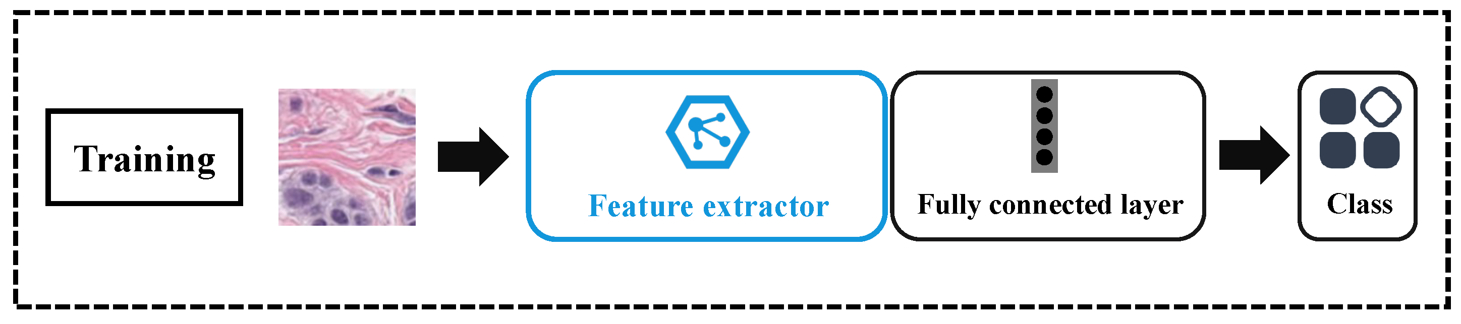
One of the drawbacks of convolutional networks is that they can only fuse local information and each pixel can only perceive its neighbors in local spatial locations, while it is more difficult to capture remote dependencies. Self-attention is a widely adopted approach for establishing non-local connections in deep learning; yet, its huge amount of operations is still a computational burden. Inspired by recent detached attention [40], we propose a lightweight single-key global spatial attention. The process of this part is shown in Figure 3. As shown in the bottom path in the figure, the input x firstly passes through a $1\times 1$ convolutional layer, which does not change the number of channels, then the global pooling downsizes the spatial dimension, after another $1\times 1$ convolutional layer, which does not change the number of channels, and the key of the input feature is finally obtained, i.e.,

$$K=Con{v}_K^{\left(2\right)}(AvgPool(Con{v}_K^{\left(1\right)}\left(x\right)))$$

(2)

Figure 3. Single-key global spatial attention. We utilize a similar idea to self-attention, but the difference is that the spatial dimension of the key collapses in our approach, and each spatially located feature has to interact with only one feature instead of interacting with all features as in self-attention. We use the idea of weighting similar to SE attention [41] to weight the important features, instead of the feature generation method in self-attention.

The middle path in Figure 3 means that passing x through a $1\times 1$ convolutional layer that allows inter-channel information exchange provides the query of the input features, i.e.,

$$Q=Con{v}_Q\left(x\right)$$

(3)

We multiply Q and K and feed the result into the Sigmoid layer to obtain the weight W for each spatial location, i.e.,

$$W=Q\times K^T$$

(4)

where T denotes the matrix transpose.

The final weighting for x is accomplished by multiplying the weight matrix W with the input features x, i.e.,

$$Out=W·x$$

(5)

In the above process, we utilized a similar idea to self-attention, but the difference is that the spatial dimension of the key collapses in our approach, and our approach does not consume huge computational resources as self-attention does, because each spatially located feature has to interact with only one feature instead of interacting with all features as in self-attention.

In addition, we used the input features themselves as the value matrix, similar to that in self-attention; however, we did not introduce the convolution for the value, which further reduces the computational effort, and we used the idea of weighting similar to SE attention [41] to weight the important features, instead of the feature generation method in self-attention.

3.4. Classification

3.4.1. Training

For training, we used cross-entropy as the loss function, i.e.,

$$L({\zeta }_i,{\widehat{\zeta }}_i)=-\sum _{i=1}^N({\zeta }_i\log {\widehat{\zeta }}_i)$$

(6)

where N is the number of categories, ${\zeta }_i$ is the ground truth distribution of the i-th category, and ${\widehat{\zeta }}_i$ is the predicted distribution of the i-th category.

3.4.2. Testing

We denote the feature extractor as $\varphi$, the feature of an input image I as $F_I=\varphi \left(I\right)$, and ${\delta }_i$ as the set of the features of the i-th category in the support set. We used the nearest class mean to obtain a center for each category, i.e.,

$${\overline{ϵ}}_j=\frac{1}{|{\delta }_i|}\sum _{FI\in {\delta }_i}{F}_I$$

(7)

The predicted category of each sample in the query set can be obtained as:

$$Category\left(F_I\right)=\arg \underset{i}{min}\left|\right|F_I-{\overline{ϵ}}_i{\left|\right|}_2$$

(8)

4. Experimental Results and Analysis

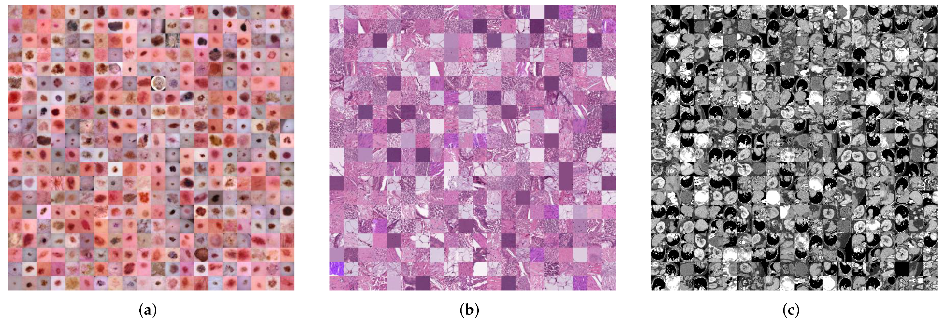
4.1. Dataset Description

The datasets employed in this paper are all from MedMNIST [42,43], which is available at https://medmnist.com/ (accessed on 31 December 2021). As a large-scale lightweight benchmark dataset for two-dimensional and three-dimensional biomedical image classification, MedMNIST has been widely used in research on medical image classification. Specifically, three datasets in MedMNIST were employed in the experiments of this paper, where the details of these datasets are presented in Figure 4 and Table 1.

Figure 4. Medical image classification datasets. (a) DermaMNIST. (b) PathMNIST. (c) OrganMNIST (Axial).

Table 1. The details of three medical image classification hldatasets.

Datasets	Classes	Training	Validation	Test	Image Modality
DermaMNIST [44,45]	7	7007	1003	2005	Dermatoscope
PathMNIST [46]	9	89,996	10,004	7180	Pathology
OrganMNIST (Axial) [47,48]	11	34,581	6491	17,778	Abdominal CT

DermaMNIST is based on HAM10000 [44,45], which is a collection of multi-source dermoscopic images of large common pigmented skin lesions. The source images with $3\times 600\times 450$ pixels were resized to $3\times 28\times 28$ pixels. The dataset consists of 10,015 dermoscopic images, which are divided into seven different diseases to form a multi-class classification task. The images were divided into a training set, verification set, and test set in the ratio of 7:1:2.

PathMNIST is based on a prior study [46] and is mainly used to predict survival in colorectal cancer histological sections. The source images with $3\times 224\times 224$ pixels were resized to $3\times 28\times 28$ pixels. In [46], a dataset (NCT-CRC-HE-100K) containing 100,000 non-overlapping image patches from hematoxylin- and eosin-stained histological images were split as 9:1 into a training set and verification set. In addition, a dataset (CRC-VAL-HE-7K) with 7180 image patches from different clinical centers was treated as the test set. The PathMNIST dataset consists of nine types of organizations, which allows for multiple classification tasks.

OrganMNIST(Axial) is the axial acquisition from 3D Computed Tomography (CT) in the Liver Tumor Segmentation Benchmark (LiTS) [47]. The organ labels in OrganMNIST (Axial) were obtained from boundary box annotations of 11 body organs in another study [48]. The original image was resized to $1\times 28\times 28$ pixels, which classifies 11 body organs into multiple categories. In detail, the training and validation set were selected from 115 and 16 CT scans in the source training set, respectively. The test set was constructed with 70 CT scans from the source test set.

4.2. Experimental Setup

For the sake of fairness, all experiments in this paper were implemented on the PyTorch framework in an NVIDIA GeForce RTX 3090. In the practical implementation, we randomly selected three categories as the training set, two categories as the validation set, and the remaining two categories as the test set in DermaMNIST, so 2-way 1-shot and 2-way 5-shot were performed in the comparative experiments. For PathMNIST, we randomly selected three categories as the training set, three categories as the validation set, and the remaining three categories as the test set. For OrganMNIST, we randomly selected five categories as the training set, three categories as the validation set, and the remaining three categories as the test set. In addition, 3-way 1-shot and 3-way 5-shot were performed in the PathMNIST and OrganMNIST. We used ResNet18 [49] as the backbone, where we added the proposed single-key global spatial attention module at the end of each convolution block. We adopted the optimizer of SGD with a momentum of 0.9. The learning rate was 0.1. We also report the $95\%$ confidence interval, and the performances were averaged over 1000 generated classification tasks.

4.3. Comparing with State-of-the-Art Algorithms

In order to quantify the superiority of our proposed algorithm, five well-known few-shot learning algorithms were selected as the comparison algorithms, including the MatchingNet [30], MAML [33], Prototype Net [31], Relation Net [50], and Transductive Propagation Network (TPN) [51].

For DermaMNIST, as can be seen from the experimental results in Table 2, our method achieved the best results on 2-way 1-shot and 5-shot. Specifically, our method outperformed the state-of-the-art method by $3.25\%$ and $1.86\%$ in 1-shot and 5-shot, respectively. We also show the loss curve and the validation accuracy curve of the proposed method on the DermaMNIST dataset, in Figure 5 and Figure 6, respectively.

Table 2. The accuracy comparison of different methods on the DermaMNIST dataset.

Method	2-Way
	1-Shot	5-Shot
MatchingNet	$55.52\pm 1.14\%$	$61.91\pm 1.57\%$
MAML	$56.14\pm 0.97\%$	$63.27\pm 1.12\%$
PrototypeNet	$56.84\pm 0.88\%$	$62.74\pm 1.18\%$
Relation Net	$58.74\pm 0.84\%$	$63.82\pm 1.20\%$
TPN	$60.12\pm 0.86\%$	$67.52\pm 1.14\%$
Ours	63.37 ± 0.80%	69.38 ± 1.03%

Figure 5. Validation accuracy curve on the DermaMNIST dataset.

Figure 6. Loss curve on the DermaMNIST dataset.

Table 3 shows the experimental results on the PathMNIST dataset; our method outperformed all existing methods. The results on the OrganMNIST dataset are shown in Table 4; our method achieved the best performance with the highest accuracy and the lowest confidence interval.

Table 3. The accuracy comparison of different methods on the PathMNIST dataset.

Method	3-Way
	1-Shot	5-Shot
MatchingNet	$46.38\pm 0.82\%$	$53.28\pm 1.29\%$
MAML	$51.58\pm 0.81\%$	$58.39\pm 0.92\%$
PrototypeNet	$51.29\pm 0.77\%$	$59.19\pm 0.82\%$
elation Net	$53.48\pm 0.81\%$	$60.73\pm 0.87\%$
TPN	$52.91\pm 0.83\%$	$59.29\pm 0.84\%$
Ours	54.82 ± 0.78%	61.92 ± 0.81%

Table 4. The accuracy comparison of different methods on the OrganMNIST dataset.

Method	3-Way
	1-Shot	5-Shot
MatchingNet	$44.59\pm 0.96\%$	$50.84\pm 1.12\%$
MAML	$48.47\pm 0.87\%$	$56.86\pm 0.96\%$
PrototypeNet	$49.39\pm 0.83\%$	$57.83\pm 0.72\%$
Relation Net	$50.93\pm 0.84\%$	$58.61\pm 0.89\%$
TPN	$51.86\pm 0.87$%	$57.35\pm 0.85\%$
Ours	53.48 ± 0.81%	59.38 ± 0.84%

4.4. Ablation Experiments

In this subsection, the ablation experiments are performed to demonstrate the effectiveness of our innovation. The ablation results on DermaMNIST, PathMNIST, and OrganMNIST are shown in Table 5, Table 6 and Table 7, respectively. Both of the proposed contributions improved the performance because collateral-type location coding allows the model to exploit feature information related to location only, while single-key global spatial attention allows the model to make each pixel in the feature map perceive global information in a cost-effective manner.

Table 5. Ablation on the DermaMNIST dataset.

Method	2-Way
	1-Shot	5-Shot
Baseline	$59.28\pm 1.01\%$	$63.81\pm 1.29\%$
+ Collateral Location Coding	$61.27\pm 0.98\%$	$65.72\pm 1.21\%$
+ Single-Key Global Spatial Attention	$62.79\pm 0.91\%$	$65.14\pm 1.18\%$
Full	63.37 ± 0.80%	69.38 ± 1.03%

Table 6. Ablation on the PathMNIST dataset.

Method	3-Way
	1-Shot	5-Shot
Baseline	$49.91\pm 0.95\%$	$56.28\pm 1.04\%$
+ Collateral Location Coding	$51.39\pm 0.91\%$	$58.21\pm 0.97\%$
+ Single-Key Global Spatial Attention	$52.96\pm 0.84\%$	$58.49\pm 0.89\%$
Full	54.82 ± 0.78%	61.92 ± 0.81%

Table 7. Ablation on the OrganMNIST dataset.

Method	3-Way
	1-Shot	5-Shot
Baseline	$50.48\pm 0.98\%$	$55.71\pm 1.07\%$
+ Collateral Location Coding	$51.41\pm 0.93\%$	$57.39\pm 0.91\%$
+ Single-Key Global Spatial Attention	$51.83\pm 0.88\%$	$57.57\pm 0.89\%$
Full	53.48 ± 0.81%	59.38 ± 0.84%

5. Conclusions

In this paper, we proposed a few-shot learning framework for medical image classification, in which we specifically proposed a collateral location encoding to help the network recognize only location-dependent features, and we proposed a single-key global spatial attention that allows the model to perceive global spatial information in a cost-effective manner. Experiments on three publicly available medical datasets confirmed the effectiveness of our algorithm. Noticing that a large amount of valuable medical data is underused, we find it urgent to fuse various medical classification data sources seeking a further boost in performance. Therefore, in our future work, we will focus on how to embed unannotated samples from different medical data sources into a few-shot learning framework to further improve model effectiveness.

References

1. Wu, Y.; Ma, W.; Gong, M.; Su, L.; Jiao, L. A novel point-matching algorithm based on fast sample consensus for image registration. IEEE Geosci. Remote Sens. Lett. 2014, 12, 43–47. [Google Scholar] [CrossRef]
2. Wu, Y.; Li, J.; Yuan, Y.; Qin, A.; Miao, Q.G.; Gong, M.G. Commonality autoencoder: Learning common features for change detection from heterogeneous images. IEEE Trans. Neural Netw. Learn. Syst. 2021, 1–14. [Google Scholar] [CrossRef] [PubMed]
3. Li, J.; Li, H.; Liu, Y.; Gong, M. Multi-fidelity evolutionary multitasking optimization for hyperspectral endmember extraction. Appl. Soft Comput. 2021, 111, 107713. [Google Scholar] [CrossRef]
4. Gong, M.; Liang, Y.; Shi, J.; Ma, W.; Ma, J. Fuzzy c-means clustering with local information and kernel metric for image segmentation. IEEE Trans. Image Process. 2012, 22, 573–584. [Google Scholar] [CrossRef] [PubMed]
5. Gong, M.; Zhou, Z.; Ma, J. Change detection in synthetic aperture radar images based on image fusion and fuzzy clustering. IEEE Trans. Image Process. 2011, 21, 2141–2151. [Google Scholar] [CrossRef]
6. Gong, M.; Feng, K.y.; Fei, X.; Qin, A.K.; Li, H.; Wu, Y. An Automatically Layer-wise Searching Strategy for Channel Pruning Based on Task-driven Sparsity Optimization. IEEE Trans. Circ. Syst. Video Technol. 2022, 1. [Google Scholar] [CrossRef]
7. Wu, Y.; Liu, J.W.; Zhu, C.Z.; Bai, Z.F.; Miao, Q.G.; Ma, W.P.; Gong, M.G. Computational intelligence in remote sensing image registration: A survey. Int. J. Autom. Comput. 2021, 18, 1–17. [Google Scholar] [CrossRef]
8. Wu, Y.; Mu, G.; Qin, C.; Miao, Q.; Ma, W.; Zhang, X. Semi-supervised hyperspectral image classification via spatial-regulated self-training. Remote Sens. 2020, 12, 159. [Google Scholar] [CrossRef] [Green Version]
9. Wu, Y.; Xiao, Z.; Liu, S.; Miao, Q.; Ma, W.; Gong, M.; Xie, F.; Zhang, Y. A Two-Step Method for Remote Sensing Images Registration Based on Local and Global Constraints. IEEE J. Sel. Top. Appl. Earth Obs. Remote Sens. 2021, 14, 5194–5206. [Google Scholar] [CrossRef]
10. Li, H.; Li, J.; Zhao, Y.; Gong, M.; Zhang, Y.; Liu, T. Cost-Sensitive Self-Paced Learning With Adaptive Regularization for Classification of Image Time Series. IEEE J. Sel. Top. Appl. Earth Obs. Remote Sens. 2021, 14, 11713–11727. [Google Scholar] [CrossRef]
11. Wang, Z.; Li, J.; Liu, Y.; Xie, F.; Li, P. An Adaptive Surrogate-Assisted Endmember Extraction Framework Based on Intelligent Optimization Algorithms for Hyperspectral Remote Sensing Images. Remote Sens. 2022, 14, 892. [Google Scholar] [CrossRef]
12. García Seco de Herrera, A.; Markonis, D.; Joyseeree, R.; Schaer, R.; Foncubierta-Rodríguez, A.; Müller, H. Semi–supervised learning for image modality classification. In International Workshop on Multimodal Retrieval in the Medical Domain; Springer: Berlin, Germany, 2015. [Google Scholar]
13. Peikari, M.; Salama, S.; Nofech-Mozes, S.; Martel, A.L. A cluster-then-label semi-supervised learning approach for pathology image classification. Sci. Rep. 2018, 8, 7193. [Google Scholar] [CrossRef] [PubMed] [Green Version]
14. Lecouat, B.; Chang, K.; Foo, C.S.; Unnikrishnan, B.; Brown, J.M.; Zenati, H.; Beers, A.; Chandrasekhar, V.; Kalpathy-Cramer, J.; Krishnaswamy, P. Semi-supervised deep learning for abnormality classification in retinal images. arXiv 2018, arXiv:1812.07832. [Google Scholar]
15. Springenberg, J.T. Unsupervised and semi-supervised learning with categorical generative adversarial networks. arXiv 2015, arXiv:1511.06390. [Google Scholar]
16. Madani, A.; Moradi, M.; Karargyris, A.; Syeda-Mahmood, T. Semi-supervised learning with generative adversarial networks for chest X-ray classification with ability of data domain adaptation. In Proceedings of the 2018 IEEE 15th International Symposium on Biomedical Imaging (ISBI 2018), Washington, DC, USA, 4–7 April 2018; pp. 1038–1042. [Google Scholar]
17. Armato, S.G.; Li, F.; Giger, M.L.; MacMahon, H.; Sone, S.; Doi, K. Lung cancer: Performance of automated lung nodule detection applied to cancers missed in a CT screening program. Radiology 2002, 225, 685–692. [Google Scholar] [CrossRef] [PubMed]
18. Liu, Q.; Yu, L.; Luo, L.; Dou, Q.; Heng, P.A. Semi-Supervised Medical Image Classification With Relation-Driven Self-Ensembling Model. IEEE Trans. Med. Imaging 2020, 39, 3429–3440. [Google Scholar] [CrossRef]
19. Gyawali, P.K.; Ghimire, S.; Bajracharya, P.; Li, Z.; Wang, L. Semi-supervised medical image classification with global latent mixing. In International Conference on Medical Image Computing and Computer-Assisted Intervention; Springer: Cham, Switzerland, 2020; pp. 604–613. [Google Scholar]
20. Phan, H.; Krawczyk-Becker, M.; Gerkmann, T.; Mertins, A. DNN and CNN with weighted and multi-task loss functions for audio event detection. arXiv 2017, arXiv:1708.03211. [Google Scholar]
21. Khan, S.H.; Hayat, M.; Bennamoun, M.; Sohel, F.A.; Togneri, R. Cost-sensitive learning of deep feature representations from imbalanced data. IEEE Trans. Neural Netw. Learn. Syst. 2017, 29, 3573–3587. [Google Scholar]
22. Han, W.; Huang, Z.; Li, S.; Jia, Y. Distribution-sensitive unbalanced data oversampling method for medical diagnosis. J. Med Syst. 2019, 43, 1–10. [Google Scholar] [CrossRef]
23. Yu, H.; Sun, C.; Yang, X.; Yang, W.; Shen, J.; Qi, Y. ODOC-ELM: Optimal decision outputs compensation-based extreme learning machine for classifying imbalanced data. Knowl. Based Syst. 2016, 92, 55–70. [Google Scholar] [CrossRef]
24. Li, C.H.; Yuen, P.C. Semi-supervised learning in medical image database. In Pacific-Asia Conference on Knowledge Discovery and Data Mining; Springer: Berlin, Germany, 2001; pp. 154–160. [Google Scholar]
25. Cubuk, E.D.; Zoph, B.; Shlens, J.; Le, Q.V. Randaugment: Practical automated data augmentation with a reduced search space. In Proceedings of the IEEE/CVF Conference on Computer Vision and Pattern Recognition Workshops, Seattle, WA, USA, 14–19 June 2020; pp. 702–703. [Google Scholar]
26. Su, H.; Shi, X.; Cai, J.; Yang, L. Local and global consistency regularized mean teacher for semi-supervised nuclei classification. In International Conference on Medical Image Computing and Computer-Assisted Intervention; Springer: Cham, Switzerland, 2019; pp. 559–567. [Google Scholar]
27. Goodfellow, I.; Pouget-Abadie, J.; Mirza, M.; Xu, B.; Warde-Farley, D.; Ozair, S.; Courville, A.; Bengio, Y. Generative adversarial nets. In Proceedings of the 28th Conference on Neural Information Processing Systems (NIPS 2014), Montreal, QC, Canada, 8–13 December 2014; p. 27. [Google Scholar]
28. Antoniou, A.; Storkey, A.; Edwards, H. Data augmentation generative adversarial networks. arXiv 2017, arXiv:1711.04340. [Google Scholar]
29. Chen, Z.; Fu, Y.; Chen, K.; Jiang, Y.G. Image block augmentation for one-shot learning. Proc. AAAI Conf. Artif. Intell. 2019, 33, 3379–3386. [Google Scholar] [CrossRef] [Green Version]
30. Vinyals, O.; Blundell, C.; Lillicrap, T.; Wierstra, D. Matching networks for one shot learning. In Proceedings of the 30th Conference on Neural Information Processing Systems (NIPS 2016), Barcelona, Spain, 5–10 December 2016; p. 29. [Google Scholar]
31. Snell, J.; Swersky, K.; Zemel, R. Prototypical networks for few-shot learning. In Proceedings of the 31st Conference on Neural Information Processing Systems (NIPS 2017), Long Beach, CA, USA, 4–9 December 2017; p. 30. [Google Scholar]
32. Li, W.; Xu, J.; Huo, J.; Wang, L.; Gao, Y.; Luo, J. Distribution consistency based covariance metric networks for few-shot learning. Proc. AAAI Conf. Artif. Intell. 2019, 33, 8642–8649. [Google Scholar] [CrossRef]
33. Finn, C.; Abbeel, P.; Levine, S. Model-agnostic meta-learning for fast adaptation of deep networks. In Proceedings of the 34th International Conference on Machine Learning, Sydney, Australia, 6–11 August 2017; pp. 1126–1135. [Google Scholar]
34. Ravi, S.; Larochelle, H. Optimization as a model for few-shot learning. In Proceedings of the 34th International Conference on Machine Learning, Sydney, Australia, 6–11 August 2017; pp. 1–11. [Google Scholar]
35. Cheng, Y.; Yu, M.; Guo, X.; Zhou, B. Few-shot learning with meta metric learners. arXiv 2019, arXiv:1901.09890. [Google Scholar]
36. Islam, M.A.; Jia, S.; Bruce, N.D. How much position information do convolutional neural networks encode? arXiv 2020, arXiv:2001.08248. [Google Scholar]
37. Wang, X.; Kong, T.; Shen, C.; Jiang, Y.; Li, L. Solo: Segmenting objects by locations. In European Conference on Computer Vision; Springer: Berlin, Germany, 2020; pp. 649–665. [Google Scholar]
38. Gonzalez, J.L.; Kim, M. PLADE-Net: Towards Pixel-Level Accuracy for Self-Supervised Single-View Depth Estimation with Neural Positional Encoding and Distilled Matting Loss. In Proceedings of the IEEE/CVF Conference on Computer Vision and Pattern Recognition, Nashville, TN, USA, 20–25 June 2021; pp. 6851–6860. [Google Scholar]
39. Hendrycks, D.; Gimpel, K. Gaussian error linear units (gelus). arXiv 2016, arXiv:1606.08415. [Google Scholar]
40. Liu, H.; Liu, F.; Fan, X.; Huang, D. Polarized self-attention: Towards high-quality pixel-wise regression. arXiv 2021, arXiv:2107.00782. [Google Scholar]
41. Hu, J.; Shen, L.; Sun, G. Squeeze-and-excitation networks. In Proceedings of the IEEE Conference on Computer Vision and Pattern Recognition, Salt Lake City, UT, USA, 18–23 June 2018; pp. 7132–7141. [Google Scholar]
42. Yang, J.; Shi, R.; Ni, B. MedMNIST Classification Decathlon: A Lightweight AutoML Benchmark for Medical Image Analysis. In Proceedings of the 2021 IEEE 18th International Symposium on Biomedical Imaging (ISBI), Nice, France, 13–16 April 2021; pp. 191–195. [Google Scholar]
43. Yang, J.; Shi, R.; Wei, D.; Liu, Z.; Zhao, L.; Ke, B.; Pfister, H.; Ni, B. MedMNIST v2: A Large-Scale Lightweight Benchmark for 2D and 3D Biomedical Image Classification. arXiv 2021, arXiv:2110.14795. [Google Scholar]
44. Tschandl, P.; Rosendahl, C.; Kittler, H. The HAM10000 dataset, a large collection of multi-source dermatoscopic images of common pigmented skin lesions. Sci. Data 2018, 5, 180161. [Google Scholar] [CrossRef]
45. Codella, N.; Rotemberg, V.; Tschandl, P.; Celebi, M.E.; Dusza, S.; Gutman, D.; Helba, B.; Kalloo, A.; Liopyris, K.; Marchetti, M.; et al. Skin lesion analysis toward melanoma detection 2018: A challenge hosted by the international skin imaging collaboration (isic). arXiv 2019, arXiv:1902.03368. [Google Scholar]
46. Kather, J.N.; Krisam, J.; Charoentong, P.; Luedde, T.; Herpel, E.; Weis, C.A.; Gaiser, T.; Marx, A.; Valous, N.A.; Ferber, D.; et al. Predicting survival from colorectal cancer histology slides using deep learning: A retrospective multicenter study. PLoS Med. 2019, 16, e1002730. [Google Scholar] [CrossRef] [PubMed]
47. Bilic, P.; Christ, P.F.; Vorontsov, E.; Chlebus, G.; Chen, H.; Dou, Q.; Fu, C.W.; Han, X.; Heng, P.A.; Hesser, J.; et al. The liver tumor segmentation benchmark (lits). arXiv 2019, arXiv:1901.04056. [Google Scholar]
48. Xu, X.; Zhou, F.; Liu, B.; Fu, D.; Bai, X. Efficient Multiple Organ Localization in CT Image Using 3D Region Proposal Network. IEEE Trans. Med. Imaging 2019, 38, 1885–1898. [Google Scholar] [CrossRef] [PubMed]
49. He, K.; Zhang, X.; Ren, S.; Sun, J. Deep residual learning for image recognition. In Proceedings of the IEEE Conference on Computer Vision and Pattern Recognition, Las Vegas, NV, USA, 27–30 June 2016; pp. 770–778. [Google Scholar]
50. Sung, F.; Yang, Y.; Zhang, L.; Xiang, T.; Torr, P.H.; Hospedales, T.M. Learning to compare: Relation network for few-shot learning. In Proceedings of the IEEE Conference on Computer Vision and Pattern Recognition, Salt Lake City, UT, USA, 18–23 June 2018; pp. 1199–1208. [Google Scholar]
51. Liu, Y.; Lee, J.; Park, M.; Kim, S.; Yang, E.; Hwang, S.J.; Yang, Y. Learning to propagate labels: Transductive propagation network for few-shot learning. In Proceedings of the International Conference on Learning Representations, New Orleans, LA, USA, 6–9 May 2019; pp. 1–14. [Google Scholar]
Publisher’s Note: MDPI stays neutral with regard to jurisdictional claims in published maps and institutional affiliations.
Article Metrics
Citations
Article Access Statistics
Multiple requests from the same IP address are counted as one view.