
Evolutionary Optimization Based Set Joint Integrated Probabilistic Data Association Filter


Abstract
:1. Introduction
- (1)
- Although the JIPDA filter is effective for automatic MTT, few improvements have been proposed to overcome its coalescence problem. We propose to optimize the posterior density of the JIPDA filter using the RFS theory, when target identity is irrelevant.
- (2)
- To the best of our knowledge, this is the first work to use the computational intelligence technique to improve the performance of the data association based filter. We model the optimization of the posterior density as an evolutionary optimization problem, improving the accuracy of the state estimation.
- (3)
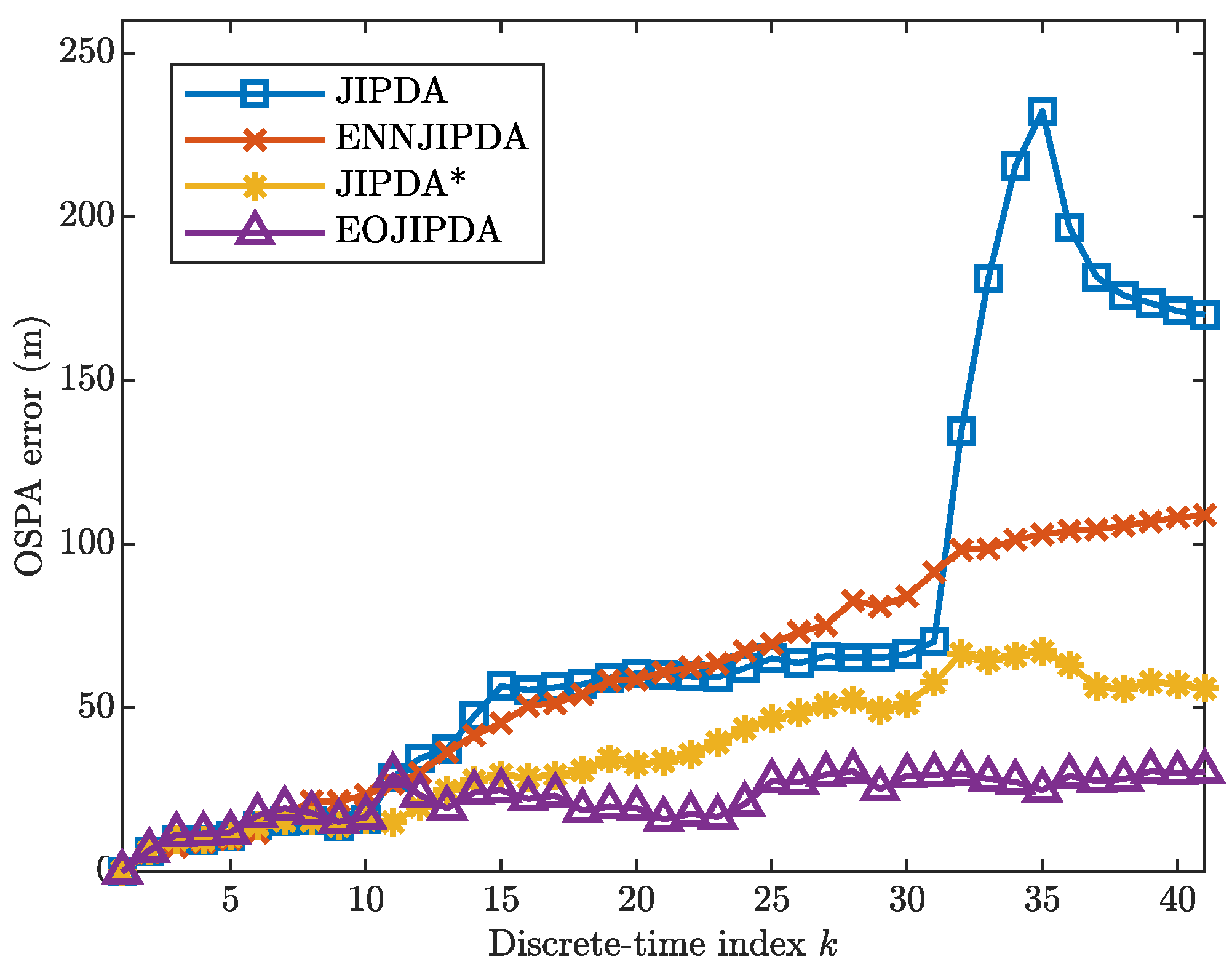
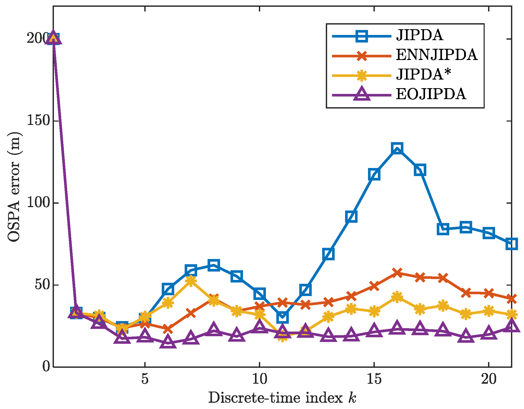
- The illustrative example shows that the EOJIPDA filter can effectively improve the accuracy of the state estimation. Simulation results obtained from two challenging MTT scenarios demonstrate the effectiveness of the EOJIPDA filter in terms of the optimal sub-pattern assignment (OSPA) multi-target miss distance.
2. Related Work
3. Background
3.1. Target and Measurement Assumptions
3.2. Joint Integrated Probabilistic Data Association Filter
- Step 1: Predicting the target state , the covariance , and the probability of target existence for each track t.
- Step 2: The tracking gate is generated for each target to select the validated measurements.
- Step 3: Association hypothesis events are formed by associating the validated measurements with the tracks.
- Step 4: The target existence probability, the target state, and the error covariance for track is approximated as [11]
4. Evolutionary-Optimization-Based Joint Integrated Probabilistic Data Association
4.1. Motivations
4.2. Evolutionary Optimization of the Posterior Density
- Step 1: It is necessary to generate the initial population for the evolutionary optimization.
- Step 2: The value of the cost function forms the fitness value for each solution.
- Step 3: The offspring solutions are generated using the selection, crossover and mutation operators.
- Step 4: Back to Step 3 and the cycle repeats.
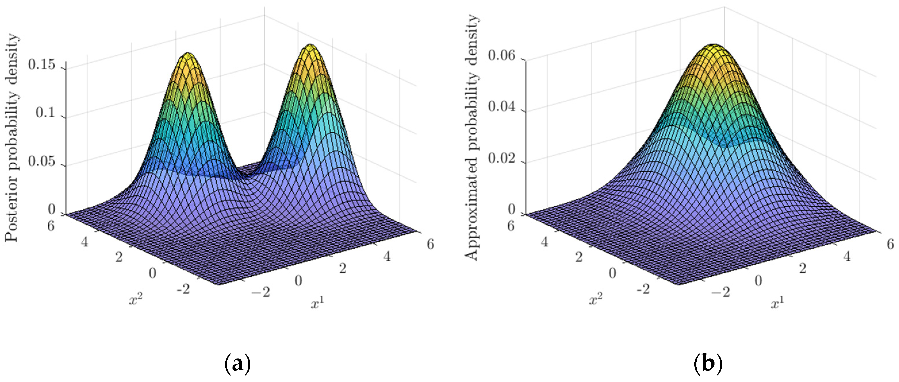
4.3. Illustrative Example
5. Numerical Simulation and Results
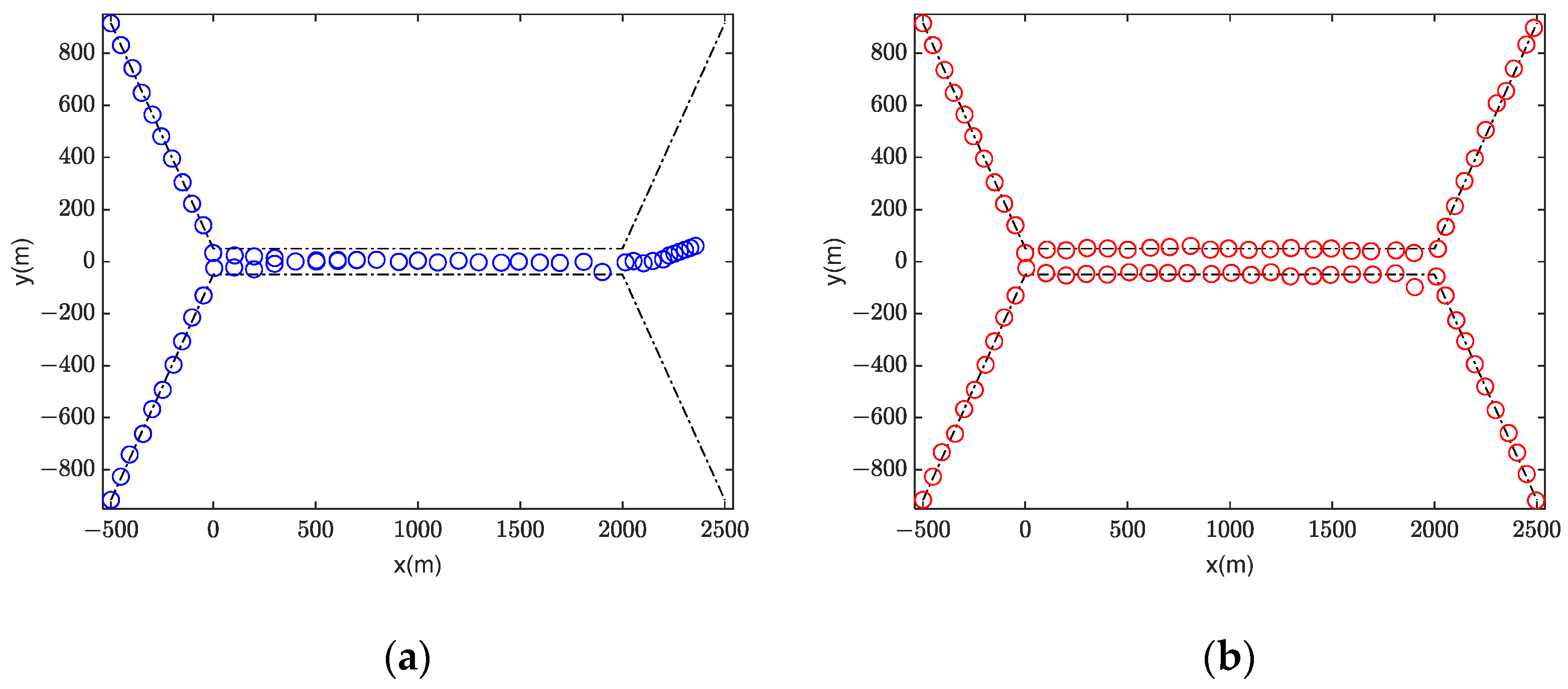
5.1. Scenario 1
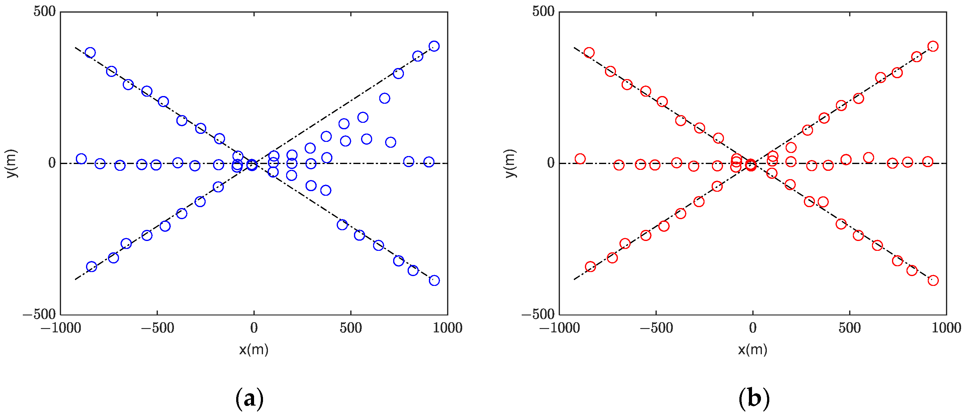
5.2. Scenario 2
6. Conclusions
Author Contributions
Funding
Data Availability Statement
Acknowledgments
Conflicts of Interest
Abbreviations
| MTT | multi-target tracking |
| MHT | multiple hypothesis tracking |
| JPDA | joint probabilistic data association |
| ENNJPDA | exact nearest-neighbor JPDA |
| ENNJIPDA | exact nearest-neighbor JIPDA |
| SJPDA | set JPDA |
| NNSJPDA | nearest-neighbor SJPDA |
| JIPDA | joint integrated probabilistic data association |
| FISST | finite set statistics |
| PHD | probability hypothesis density |
| CPHD | cardinalized PHD |
| MB | multi-Bernoulli |
| LMB | label multi-Bernoulli |
| GLMB | generalized label multi-Bernoulli |
| RFS | random finite set |
| GM | Gaussian mixture |
| SMC | sequential Monte Carlo |
| EOJIPDA | joint integrated probabilistic data association |
| OSPA | optimal sub-pattern assignment |
| List of mathematical symbols | |
| state vector at time k | |
| transition matrix at time k | |
| Gaussian probability density with mean and covariance | |
| measurement vector at time k | |
| observation matrix at time k | |
| detection probability | |
| covariance matrix at time k | |
| target existence probability at time k | |
| , | Markov chain coefficients |
| predicted measurement vector from time k-1 to time k | |
| innovation covariance | |
| measurement dimension | |
| G | gating threshold |
| association hypothesis event | |
| gating probability | |
| cluster volume | |
| filter gain | |
| number of all association hypothesis events | |
| trace for the covariance matrix | |
References
- Anjos, J.C.S.D.; Gross, J.L.G.; Matteussi, K.J.; González, G.V.; Geyer, C.F.R. An algorithm to minimize energy consumption and elapsed time for IoT workloads in a hybrid architecture. Sensors 2021, 21, 2914. [Google Scholar] [CrossRef] [PubMed]
- Martins, J.A.; Ochôa, I.S.; Silva, L.A.; Mendes, A.S.; González, G.V.; Santana, J.D.; Leithardt, V.R.Q. PRIPRO: A comparison of classification algorithms for managing receiving notifications in smart environments. Appl. Sci. 2020, 10, 502. [Google Scholar] [CrossRef] [Green Version]
- Baser, E.; McDonald, M.; Kirubarajan, T.; Efe, M. A joint multitarget estimator for the joint target detection and tracking filter. IEEE Trans. Signal Process. 2015, 63, 3857–3871. [Google Scholar] [CrossRef]
- Mallick, M.; Vo, B.N.; Kirubarajan, T.; Arulampalam, S. Introduction to the issue on multitarget tracking. IEEE J. Sel. Top. Signal Process. 2013, 7, 373–375. [Google Scholar] [CrossRef]
- Severson, T.A.; Paley, D.A. Distributed multitarget search and track assignment with consensus based coordination. IEEE Sens. J. 2015, 15, 864–875. [Google Scholar] [CrossRef]
- Reid, D. An algorithm for tracking multiple targets. IEEE Trans. Autom. Cont. 1979, 24, 843–854. [Google Scholar] [CrossRef]
- Kurien, T. Issues in the design of practical multitarget tracking algorithms. In Multitarget-Multisensor Tracking: Advanced Applications; Bar-Shalom, Y., Ed.; Artech House: Norwood, MA, USA, 1990; pp. 43–83. [Google Scholar]
- Fortmann, T.E.; Bar-Shalom, Y.; Scheffe, M. Sonar tracking of multiple targets using joint probabilistic data association. IEEE J. Ocean. Eng. 1983, 8, 173–184. [Google Scholar] [CrossRef] [Green Version]
- Mušicki, D.; Evans, R. Joint integrated probabilistic data association: JIPDA. IEEE Trans. Aerosp. Electron. Syst. 2004, 40, 1093–1099. [Google Scholar] [CrossRef]
- Svensson, L.; Svensson, D.; Guerriero, M.; Willett, P. Set JPDA filter for multitarget tracking. IEEE Trans. Signal Process. 2011, 59, 4677–4691. [Google Scholar] [CrossRef] [Green Version]
- Zhu, Y.; Wang, J.; Liang, S.; Wang, J. Covariance control joint integrated probabilistic data association filter for multi-target tracking. IET Radar Sonar Nav. 2019, 13, 584–592. [Google Scholar] [CrossRef]
- Fitzgerald, R.J. Development of practical PDA logic for multitarget tracking by microprocessor. In Multitarget-Multisensor Tracking: Advanced Applications; Bar-Shalom, Y., Ed.; Artech House: Norwood, MA, USA, 1990; pp. 1–23. [Google Scholar]
- Blom, H.; Bloem, E. Probabilistic data association avoiding track coalescence. IEEE Trans. Autom. Cont. 2000, 45, 247–259. [Google Scholar] [CrossRef]
- Zhu, Y.; Wang, J.; Liang, S. Efficient joint probabilistic data association filter based on Kullback-Leibler divergence for multi-target tracking. IET Radar Sonar Nav. 2017, 11, 1540–1548. [Google Scholar] [CrossRef]
- Zhu, Y.; Liang, S.; Wu, X.J.; Yang, H.H. A random finite set based joint probabilistic data association filter with non-homogeneous Markov chain. Front. Inf. Technol. Electron. Eng. 2021, 22, 1114–1126. [Google Scholar] [CrossRef]
- Blom, H.; Bloem, E.; Mušicki, D. JIPDA*: Automatic target tracking avoiding track coalescence. IEEE Trans. Aerosp. Electron. Syst. 2015, 51, 962–974. [Google Scholar] [CrossRef]
- Mahler, R. Statistical Multisource Multitarget Information Fusion; Artech House: Norwood, MA, USA, 2007. [Google Scholar]
- Mahler, R. Multitarget Bayes filtering via first-order multitarget moments. IEEE Trans. Aerosp. Electron. Syst. 2003, 39, 1152–1178. [Google Scholar] [CrossRef]
- Mahler, R. PHD filters of higher order in target number. IEEE Trans. Aerosp. Electron. Syst. 2007, 43, 1523–1543. [Google Scholar] [CrossRef]
- Vo, B.T.; Vo, B.N.; Cantoni, A. The cardinality balanced multi-target multi-Bernoulli filter and its implementations. IEEE Trans. Signal Process. 2009, 57, 409–423. [Google Scholar] [CrossRef] [Green Version]
- Reuter, S.; Vo, B.T.; Vo, B.N.; Dietmayer, K. The labeled multi-Bernoulli filter. IEEE Trans. Signal Process. 2014, 62, 3246–3260. [Google Scholar] [CrossRef]
- Vo, B.N.; Vo, B.T.; Phung, D. Labeled random finite sets and the Bayes multi-target tracking filter. IEEE Trans. Signal Process. 2014, 62, 6554–6567. [Google Scholar] [CrossRef] [Green Version]
- Vo, B.T.; Vo, B.N. Labeled random finite sets and multi-target conjugate priors. IEEE Trans. Signal Process. 2013, 61, 3460–3475. [Google Scholar] [CrossRef]
- Blackman, S.; Popoli, R. Design and Analysis of Modern Tracking Systems; Artech House: Norwood, MA, USA, 1999. [Google Scholar]
- Breidt, F.J.; Carriquiry, A.L. Highest density gates for target tracking. IEEE Trans. Aerosp. Electron. Syst. 2000, 36, 47–55. [Google Scholar] [CrossRef]
- Abraham, A.; Nedjah, N.; Mourelle, L.M. Evolutionary computation: From genetic algorithms to genetic programming. In Genetic Systems Programming: Theory and Experiences; Springer: Berlin/Heidelberg, Germany, 2006; Volume 13, pp. 1–20. [Google Scholar] [CrossRef]
- Gong, M.G.; Li, H.; Meng, D.Y.; Miao, Q.G. Decomposition-Based Evolutionary Multi-objective Optimization to Self-paced Learning. IEEE Trans. Evolut. Comput. 2019, 23, 288–302. [Google Scholar] [CrossRef]
- Bar-Shalom, Y.; Chang, K.C.; Blom, H.A.P. Automatic Track Formation in Clutter with a Recursive Algorithm. Multitarget-Multisensor Tracking; Artech House: Norwood, MA, USA, 1990; pp. 25–42. [Google Scholar]
- Schuhmacher, D.; Vo, B.T.; Vo, B.N. A consistent metric for performance evaluation of multi-object filters. IEEE Trans. Signal Process. 2008, 56, 3447–3457. [Google Scholar] [CrossRef] [Green Version]
- Zhu, Y.; Wang, J.; Liang, S. Multi-Objective Optimization Based Multi-Bernoulli Sensor Selection for Multi-Target Tracking. Sensors 2019, 19, 980. [Google Scholar] [CrossRef] [PubMed] [Green Version]


| JPDA-Based Multi-Target Tracking | ||
| Reference | Filter | Characteristic |
| [8] | JPDA | The number of targets and their initial states are known a priori. The number of targets remains constant during tracking. |
| [12] | ENNJPDA | After a measurement-to-target assignment is performed, tracks are only updated by a single measurement. |
| [13] | JPDA* | The best data association hypothesis is chosen to calculate the measurement-to-target probabilities. |
| [10] | SJIPDA | When all hypotheses are combined together for full optimization, the computation burden can be huge. |
| [10] | KLSJPDA | The optimal Gaussian approximations are provided in the Kullback–Leibler sense. |
| [14] | MOJPDA | The cost function is a linear combination of multiple objective functions. |
| [15] | NNSJPDA | A pair selection criterion is used for the iterative optimization. |
| JIPDA-Based Multi-Target Tracking | ||
| Reference | Filter | Characteristic |
| [9] | JIPDA | The number of targets can be unknown and time-varying. Measurements are used to initiate tracks. |
| [16] | JIPDA* | It combines the JIPDA filter with the JPDA* scheme. The hypothesis events being pruned may contain some useful information. |
| [11] | CCJIPDA | It strongly depends on initializations and improper initializations may result in bad local minima. |
| RFS Based Algorithms | ||
| Reference | Filter | Characteristic |
| [18] | PHD | Moment approximation of the Bayes multi-target filter. It has no analytical expression for the posterior multi-target density. |
| [19] | CPHD | Besides the moment approximation, the filter also propogates the cardinality distribution. |
| [20] | MB | A set of multi-Bernoulli parameters are used to characterize the posterior multi-target RFS. |
| [21] | LMB | A generalization of the multi-Bernoulli filter. |
| [22,23] | GLMB | The GLMB density is closed under the multi-target prediction and update operations. |
| Clutter Rate | JIPDA | ENNJIPDA | JIPDA* | EOJIPDA |
|---|---|---|---|---|
| r = 3 | 241 | 287 | 293 | 299 |
| r = 6 | 238 | 281 | 290 | 297 |
| r = 9 | 230 | 279 | 283 | 294 |
Publisher’s Note: MDPI stays neutral with regard to jurisdictional claims in published maps and institutional affiliations. |
© 2022 by the authors. Licensee MDPI, Basel, Switzerland. This article is an open access article distributed under the terms and conditions of the Creative Commons Attribution (CC BY) license (https://creativecommons.org/licenses/by/4.0/).
Share and Cite
Liang, S.; Zhu, Y.; Li, H. Evolutionary Optimization Based Set Joint Integrated Probabilistic Data Association Filter. Electronics 2022, 11, 582. https://doi.org/10.3390/electronics11040582
Liang S, Zhu Y, Li H. Evolutionary Optimization Based Set Joint Integrated Probabilistic Data Association Filter. Electronics. 2022; 11(4):582. https://doi.org/10.3390/electronics11040582
Chicago/Turabian StyleLiang, Shuang, Yun Zhu, and Hao Li. 2022. "Evolutionary Optimization Based Set Joint Integrated Probabilistic Data Association Filter" Electronics 11, no. 4: 582. https://doi.org/10.3390/electronics11040582
APA StyleLiang, S., Zhu, Y., & Li, H. (2022). Evolutionary Optimization Based Set Joint Integrated Probabilistic Data Association Filter. Electronics, 11(4), 582. https://doi.org/10.3390/electronics11040582