
Business Process Outcome Prediction Based on Deep Latent Factor Model


Abstract
:1. Introduction
2. Related Works
3. Preliminaries
3.1. Event Log
3.2. Latent Factor Model
4. Deep Latent Factor Model for Predicting the Outcome
- 1.
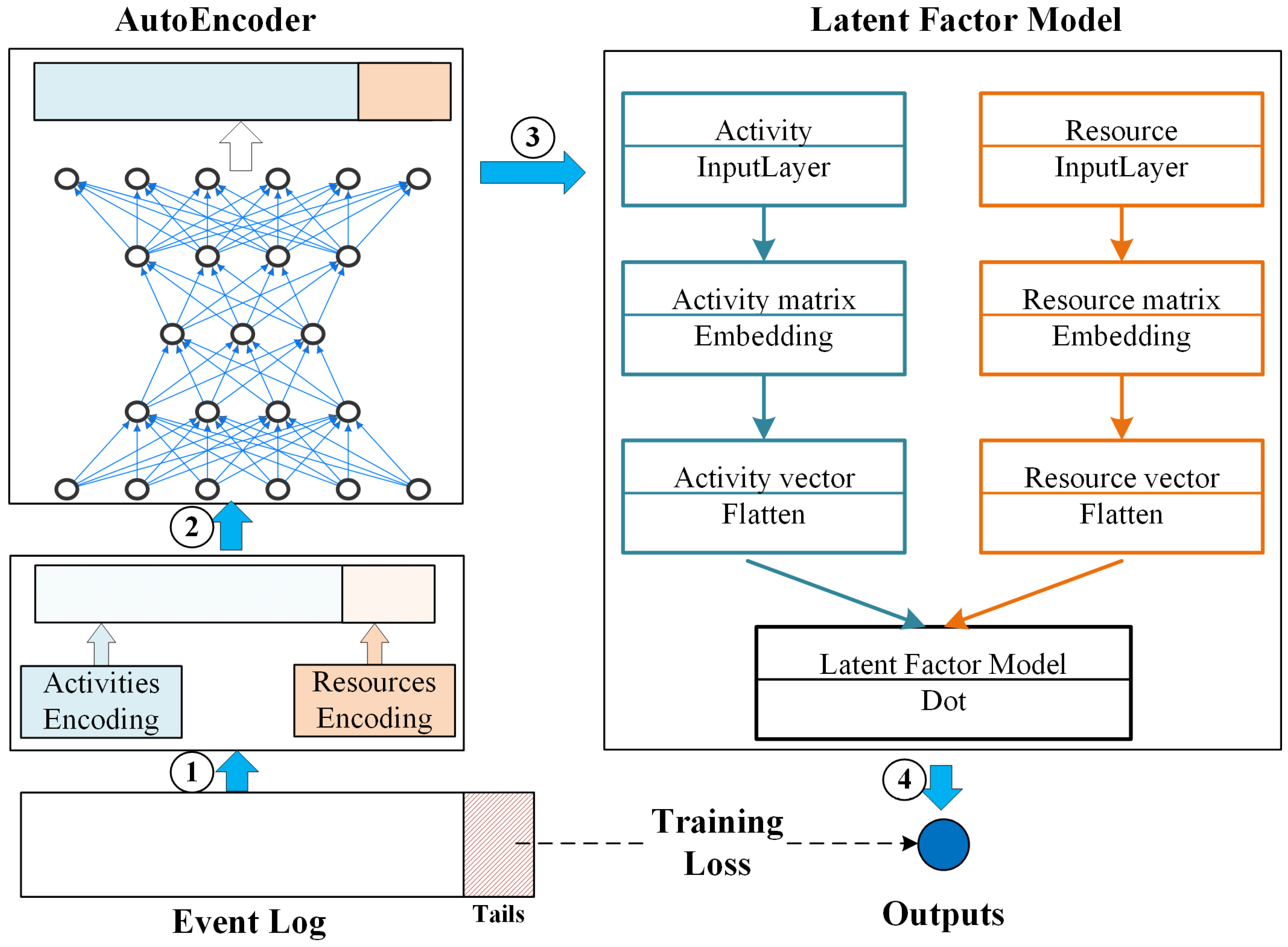
- Preprocess logs in the offline phase.In Section 4.1, we preprocess the historical event logs and construct the case–event matrix.Then, in Section 4.2, we use the self-encoder to reduce its dimensionality.
- 2.
- Predict event flow in the online phase.In Section 4.3, we construct and train latent factor models based on matrix decomposition techniques and gradient descent methods.Finally, in Section 4.4, the model is used to run the real-time prediction of event streams.
4.1. Constructing the Input Log Vector
| Algorithm 1: Construction of behavior vector |
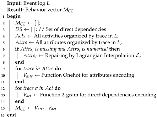 |
4.2. Vector Dimensionality Reduction Based on Stacked Autoencoder
4.3. Constructing a Deep Latent Factor Model
4.4. Predicting Process Results
5. Experiments
5.1. Experimental Setup
- 1.
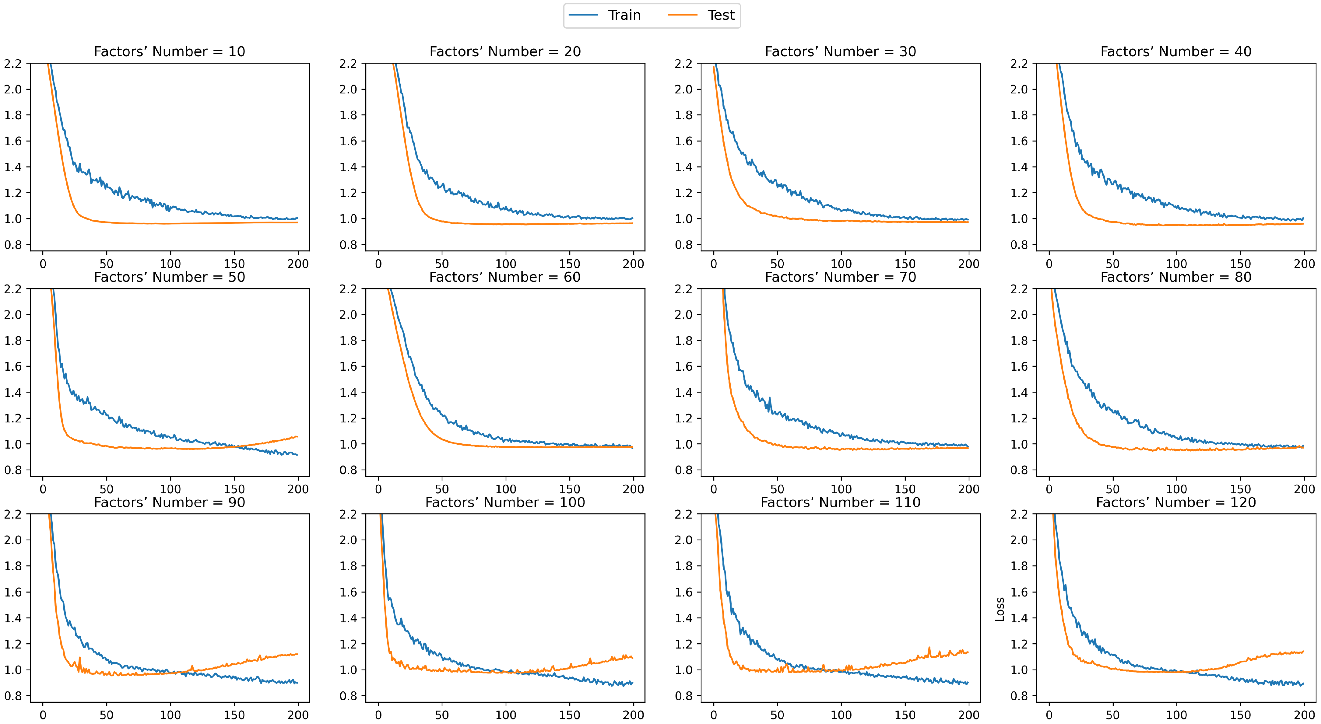
- We set different numbers of latent factors. Multiple sets of experiments analyze the prediction effects of the proposed prediction method under five logs.
- 2.
- Analysis based on different data objects. Compare the prediction results of the model when only control flow or data flow is considered with those when both control flow and data flow are considered.
- 3.
5.2. Results
5.3. Discussions
6. Conclusions
Author Contributions
Funding
Data Availability Statement
Conflicts of Interest
References
- van der Aalst, W.M.P. Process Mining: Data Science in Action, 2nd ed.; Springer: Berlin/Heidelberg, Germany, 2016. [Google Scholar] [CrossRef]
- van der Aalst, W.; Adriansyah, A.; de Medeiros, A.K.A.; Arcieri, F.; Baier, T.; Blickle, T.; Bose, J.C.; van den Brand, P.; Brandtjen, R.; Buijs, J.; et al. Process Mining Manifesto. In Proceedings of the Business Process Management Workshops; Daniel, F., Barkaoui, K., Dustdar, S., Eds.; Springer: Berlin/Heidelberg, Germany, 2012; Volume 99, pp. 169–194. [Google Scholar] [CrossRef] [Green Version]
- Teinemaa, I.; Dumas, M.; Rosa, M.L.; Maggi, F.M. Outcome-Oriented Predictive Process Monitoring: Review and Benchmark. ACM Trans. Knowl. Discov. Data 2019, 13, 1–57. [Google Scholar] [CrossRef]
- Wang, J.; Yu, D.; Liu, C.; Sun, X. Outcome-Oriented Predictive Process Monitoring with Attention-Based Bidirectional LSTM Neural Networks. In Proceedings of the 2019 IEEE International Conference on Web Services (ICWS), Milan, Italy, 8–13 July 2019. [Google Scholar] [CrossRef]
- Andreas, M.; Adrian, N. Considering Non-sequential Control Flows for Process Prediction with Recurrent Neural Networks. In Proceedings of the 2018 44th Euromicro Conference on Software Engineering and Advanced Applications (SEAA), Prague, Czech Republic, 29–31 August 2018. [Google Scholar] [CrossRef]
- Hinkka, M.; Lehto, T.; Heljanko, K.; Jung, A. Classifying Process Instances Using Recurrent Neural Networks. In Proceedings of the Business Process Management Workshops; Daniel, F., Sheng, Q.Z., Motahari, H., Eds.; Lecture Notes in Business Information Processing. Springer International Publishing: Cham, Switzerland, 2019; pp. 313–324. [Google Scholar] [CrossRef] [Green Version]
- Folino, F.; Folino, G.; Guarascio, M.; Pontieri, L. Learning Effective Neural Nets for Outcome Prediction from Partially Labelled Log Data. In Proceedings of the 2019 IEEE 31st International Conference on Tools with Artificial Intelligence (ICTAI), Portland, OR, USA, 4–6 November 2019; Volume 11, pp. 1396–1400. [Google Scholar] [CrossRef]
- Mongia, A.; Majumdar, A. Matrix Completion on Learnt Graphs: Application to Collaborative Filtering. Expert Syst. Appl. 2021, 185, 115652. [Google Scholar] [CrossRef]
- Maggi, F.M.; Di Francescomarino, C.; Dumas, M.; Ghidini, C. Predictive Monitoring of Business Processes. In Proceedings of the Advanced Information Systems Engineering; Hutchison, D., Kanade, T., Kittler, J., Kleinberg, J.M., Kobsa, A., Mattern, F., Mitchell, J.C., Naor, M., Nierstrasz, O., Pandu Rangan, C., et al., Eds.; Springer International Publishing: Cham, Switzerland, 2014; Volume 8484, pp. 457–472. [Google Scholar] [CrossRef] [Green Version]
- de Leoni, M.; van der Aalst, W.M.; Dees, M. A General Process Mining Framework for Correlating, Predicting and Clustering Dynamic Behavior Based on Event Logs. Inf. Syst. 2016, 56, 235–257. [Google Scholar] [CrossRef]
- Francescomarino, C.D.; Dumas, M.; Maggi, F.M.; Teinemaa, I. Clustering-Based Predictive Process Monitoring. IEEE Trans. Serv. Comput. 2019, 12, 896–909. [Google Scholar] [CrossRef] [Green Version]
- Leontjeva, A.; Conforti, R.; Francescomarino, C.D.; Dumas, M.; Maggi, F.M. Complex Symbolic Sequence Encodings for Predictive Monitoring of Business Processes. In Business Process Management; Proceedings; Motahari-Nezhad, H.R., Recker, J., Weidlich, M., Eds.; Lecture Notes in Computer Science; Springer: Innsbruck, Austria, 2015; Volume 9253, pp. 297–313. [Google Scholar] [CrossRef] [Green Version]
- Pasquadibisceglie, V.; Appice, A.; Castellano, G.; Malerba, D.; Modugno, G. Orange: Outcome-oriented Predictive Process Monitoring Based on Image Encoding and CNNs. IEEE Access 2020, 8, 184073–184086. [Google Scholar] [CrossRef]
- Cheng, Z.; Ding, Y.; Zhu, L.; Kankanhalli, M. Aspect-Aware Latent Factor Model: Rating Prediction with Ratings and Reviews. In Proceedings of the 2018 World Wide Web Conference on World Wide Web—WWW ’18; ACM Press: Lyon, France, 2018; pp. 639–648. [Google Scholar] [CrossRef] [Green Version]
- Wang, Q.; Chen, S.; Luo, X. An Adaptive Latent Factor Model via Particle Swarm Optimization. Neurocomputing 2019, 369, 176–184. [Google Scholar] [CrossRef]
- Luo, X.; Zhou, M.; Li, S.; Shang, M. An Inherently Nonnegative Latent Factor Model for High-Dimensional and Sparse Matrices from Industrial Applications. IEEE Trans. Ind. Inform. 2018, 14, 2011–2022. [Google Scholar] [CrossRef]
- Wu, D.; Luo, X.; Shang, M.; He, Y.; Wang, G.; Wu, X. A Data-Characteristic-Aware Latent Factor Model for Web Services QoS Prediction. IEEE Trans. Knowl. Data Eng. 2020, 34, 1. [Google Scholar] [CrossRef]
- Mongia, A.; Jhamb, N.; Chouzenoux, E.; Majumdar, A. Deep Latent Factor Model for Collaborative Filtering. Signal Process. 2020, 169, 107366. [Google Scholar] [CrossRef] [Green Version]
- Wu, D.; Luo, X.; Shang, M.; He, Y.; Wang, G.; Zhou, M. A Deep Latent Factor Model for High-Dimensional and Sparse Matrices in Recommender Systems. IEEE Trans. Syst. Man, Cybern. Syst. 2021, 51, 4285–4296. [Google Scholar] [CrossRef]
- Weinzierl, S. Exploring Gated Graph Sequence Neural Networks for Predicting Next Process Activities. In Proceedings of the Business Process Management Workshops; Marrella, A., Weber, B., Eds.; Lecture Notes in Business Information Processing. Springer International Publishing: Cham, Switzerland, 2022; pp. 30–42. [Google Scholar] [CrossRef]
- Santoso, A.; Felderer, M. Specification-Driven Predictive Business Process Monitoring. Softw. Syst. Model. 2020, 19, 1307–1343. [Google Scholar] [CrossRef] [Green Version]
- Hinkka, M.; Lehto, T.; Heljanko, K. Exploiting Event Log Event Attributes in RNN Based Prediction. In Proceedings of the New Trends in Databases and Information Systems; Welzer, T., Eder, J., Podgorelec, V., Wrembel, R., Ivanović, M., Gamper, J., Morzy, M., Tzouramanis, T., Darmont, J., Kamišalić Latifić, A., Eds.; Springer International Publishing: Cham, Switzerland, 2019; Volume 1064, pp. 405–416. [Google Scholar] [CrossRef]
- Mehdiyev, N.; Evermann, J.; Fettke, P. A Novel Business Process Prediction Model Using a Deep Learning Method. Bus. Inf. Syst. Eng. 2020, 62, 143–157. [Google Scholar] [CrossRef] [Green Version]
- Abdi, H.; Williams, L.J. Principal Component Analysis. Wiley Interdiscipl. Rev. Comput. Stat. 2010, 2, 433–459. [Google Scholar] [CrossRef]
- LeCun, Y.; Bengio, Y.; Hinton, G. Deep Learning. Nature 2015, 521, 436–444. [Google Scholar] [CrossRef] [PubMed]
- Hoang, T.C.N.; Lee, S.; Kim, J.; Ko, J.; Marco, C. Autoencoders for Improving Quality of Process Event Logs. Expert Syst. Appl. 2019, 131, 132–147. [Google Scholar] [CrossRef]
- Horiguchi, S.; Ikami, D.; Aizawa, K. Significance of Softmax-based Features in Comparison to Distance Metric Learning-based Features. IEEE Trans. Pattern Anal. Mach. Intell. 2019, 42, 1279–1285. [Google Scholar] [CrossRef] [PubMed] [Green Version]


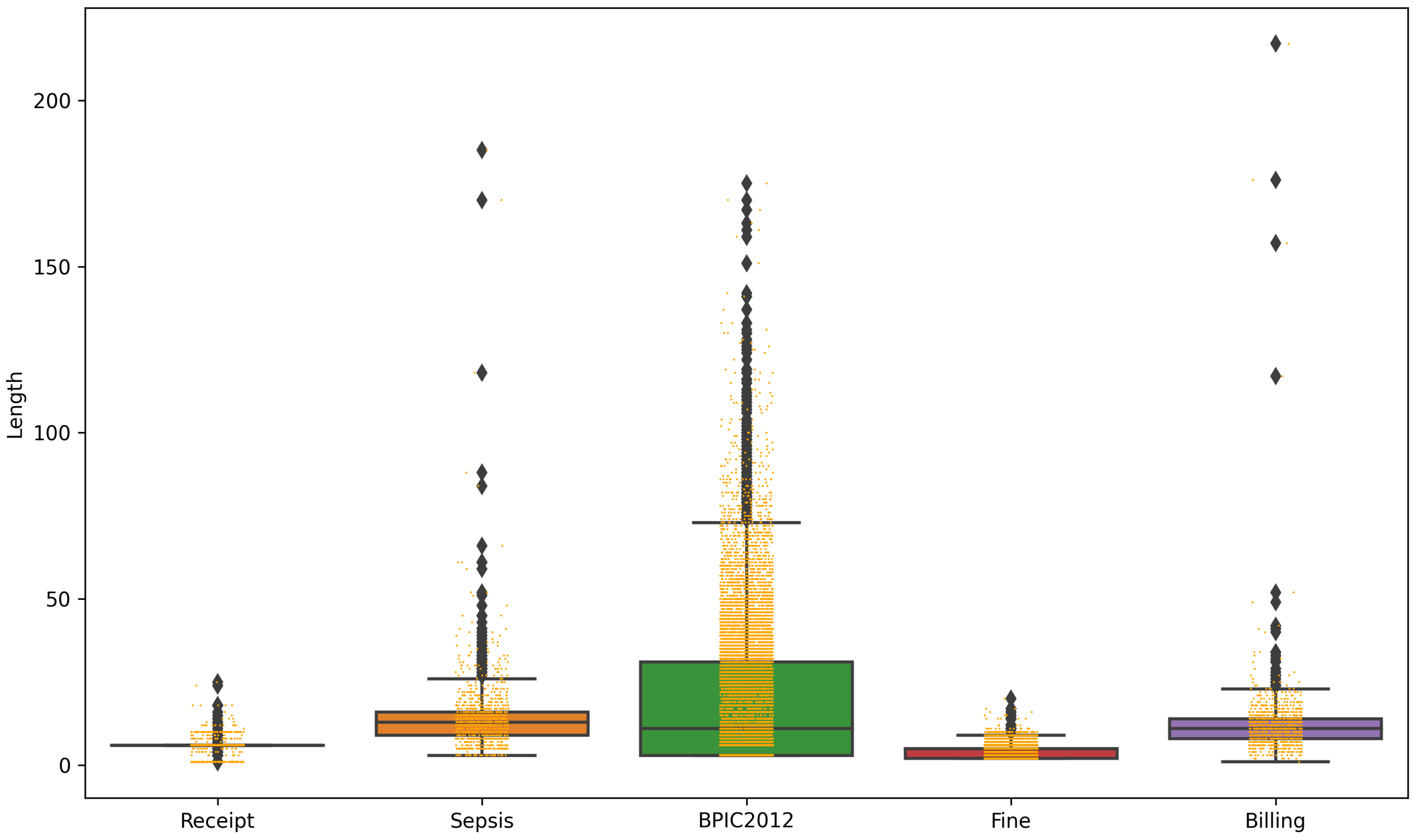
| Number | Receipt | Sepsis | BPIC2012 | Fine | Billing |
|---|---|---|---|---|---|
| Traces | 1318 | 1049 | 13,087 | 150,370 | 1013 |
| Events | 8577 | 15,214 | 262,200 | 561,470 | 12,506 |
| Activities | 27 | 16 | 36 | 11 | 18 |
| Resources | 48 | 26 | 69 | \ | \ |
| Results | 13 | 14 | 11 | 7 | 14 |
| Unique direct dependency | 99 | 115 | 125 | 70 | 142 |
| RF [3] | XGBoost [3] | Att-Bi-LSTM [4] | DLFM | ||||
|---|---|---|---|---|---|---|---|
| Factors’ Number | AUC under Control Flow | AUC under Data Flow | AUC under Double Flows | ||||
| Receipt | 0.8235 | 0.8316 | \ | 10 | 0.8611 | 0.6123 | 0.9452 |
| 50 | 0.8823 | 0.8082 | 0.9554 | ||||
| 100 | 0.9051 | 0.8125 | 0.9581 | ||||
| Sepsis | 0.8104 | 0.8412 | 0.92 | 10 | 0.7829 | 0.8374 | 0.8411 |
| 50 | 0.8469 | 0.8368 | 0.8429 | ||||
| 100 | 0.8479 | 0.8527 | 0.8548 | ||||
| BPIC2012 | 0.7126 | 0.7121 | 0.85 | 10 | 0.7930 | 0.7876 | 0.7978 |
| 50 | 0.7782 | 0.7848 | 0.7928 | ||||
| 100 | 0.7523 | 0.7606 | 0.7783 | ||||
| Fine | 0.8163 | 0.8232 | 0.85 | 10 | 0.9388 | \ | 0.9388 |
| 50 | 0.9391 | \ | 0.9391 | ||||
| 100 | 0.9388 | \ | 0.9388 | ||||
| Billing | 0.7761 | 0.8109 | 0.82 | 10 | 0.8856 | \ | 0.8856 |
| 50 | 0.8957 | \ | 0.8957 | ||||
| 100 | 0.9077 | \ | 0.9077 | ||||
Publisher’s Note: MDPI stays neutral with regard to jurisdictional claims in published maps and institutional affiliations. |
© 2022 by the authors. Licensee MDPI, Basel, Switzerland. This article is an open access article distributed under the terms and conditions of the Creative Commons Attribution (CC BY) license (https://creativecommons.org/licenses/by/4.0/).
Share and Cite
Lu, K.; Fang, X.; Fang, X. Business Process Outcome Prediction Based on Deep Latent Factor Model. Electronics 2022, 11, 1509. https://doi.org/10.3390/electronics11091509
Lu K, Fang X, Fang X. Business Process Outcome Prediction Based on Deep Latent Factor Model. Electronics. 2022; 11(9):1509. https://doi.org/10.3390/electronics11091509
Chicago/Turabian StyleLu, Ke, Xinjian Fang, and Xianwen Fang. 2022. "Business Process Outcome Prediction Based on Deep Latent Factor Model" Electronics 11, no. 9: 1509. https://doi.org/10.3390/electronics11091509
APA StyleLu, K., Fang, X., & Fang, X. (2022). Business Process Outcome Prediction Based on Deep Latent Factor Model. Electronics, 11(9), 1509. https://doi.org/10.3390/electronics11091509