Are the Significant Ionospheric Anomalies Associated with the 2007 Great Deep-Focus Undersea Jakarta–Java Earthquake?

Abstract

This work is an attempt to critically analyze the correlation between great deep-focus undersea earthquake and possible ionospheric anomalies. The significant TEC (total electron content) temporal and spatial anomalies were detected over the epicenter of 2007 M_w7.5 Jakarta–Java earthquake, and they coincide well with the striking plasma anomalies in the ionosphere in situ observed by the LEO (low Earth orbit) satellite. The localization and synchronization of the disturbances during the earthquake suggest that these ionospheric anomalies are highly related to this large undersea earthquake. In order to identify this correlation, we made efforts to distinguish seismo-associated signals from large electromagnetic noise due to solar and geomagnetic activities, natural non-seismic sources and known artificial signals. Nevertheless, the difficulties of this work should be recognized and approached with caution. This special (deep-focus and undersea) case study here provides us with valuable information on the study of lithosphere–atmosphere–ionosphere (LAI) coupling process and reminds us that deep-focus undersea seismic events need to be treated more carefully and discreetly in the future.

1. Introduction

Over the past decades, seismic anomalies occurring during (pre-, co- and post-) large earthquakes have been widely investigated [1,2,3,4,5,6]. A large number of studies have been carried out both on ground and in space with different physical parameters and quantities, such as ionospheric TEC [7,8,9,10] and plasma [9,11,12,13], electromagnetic emissions [14,15,16,17], thermal anomalies [18,19,20,21] and particle precipitation [22,23,24], etc., and methodologies such as in situ observation [9,13,15], numerical modeling [25,26,27] and machine-learning [28,29], etc. They are essential to our understanding of the lithosphere–atmosphere–ionosphere (LAI) coupling process. Unlike the well-established co-seismic effects in the lithosphere and upper atmosphere [30,31,32,33,34,35], the possible pre- and post-seismic phenomena in the ionosphere have not been fully confirmed.

Even though many seismic anomalies have been found in the ionosphere, this physical process of LAI coupling is still unclear and even controversial, and there are still plenty of issues or details that need to be carefully worked through. On the one hand, such studies rarely distinguish between inland and submarine seismic events and mainly focus on the strong cases with a shallow focus (generally less than 100 km). For example, most of the seismic electromagnetic emission (EME) observations reported in the literature are generally associated with strong ($\mathrm{M}\ge 5.0$) shallow earthquakes [22,23,24,36]. Le et al. [37] statistically investigated 736 M6.0+ earthquakes globally during 2002–2010 association with pre-earthquake ionospheric anomalies and found that TEC anomalies were generally associated with shallow earthquakes. Xia et al. [38] also examined pre-earthquake ionospheric TEC variations in the Qinghai–Tibet region and found that the focal depth, but not magnitude, of the earthquakes would govern the occurrence of the upper/lower anomalies. In addition, for undersea earthquakes, although they have some similar characteristics to seismic activities on land in some ways, such as the increased gases and aerosol release in seismic regions and which in turn rises and affects the electromagnetic environment of the atmosphere [39,40,41,42,43,44] and seismically induced acoustic and gravity waves [26,27,45,46,47,48,49,50]. However, studies have shown that it is a bit complicated, and there are some differences. Kakinami et al. [51] analyzed TEC response to three large submarine earthquakes in Japan, Chile and Indonesia and found that TEC and plasma anomalies occurred just above the tsunami source area. Compared with the inland earthquake which directly connects with the plate tectonics, Song et al. [52] also suggest that the seismo-ionospheric effect before the offshore earthquake interacts with the seawater that results in the more extensive abnormal regions. On the other hand, it is difficult to identify the earthquake associated effects due to the fuzzy background noises resulting from natural (such as volcanic eruptions, thunderstorms, tsunamis, etc.) and artificial non-seismic sources (such as communications facilities, power lines, explosions, etc.), in addition to solar and global geomagnetic perturbations. For the above reasons, the main focus of this work is to study the possibility of ionospheric perturbations associated to a special (deep-focus and undersea) case, i.e., the 2007 $M_{w}7.5$ Jakarta–Java Earthquake. Then, we attempt to carefully eliminate background noises and critically discuss possible physical mechanisms of this lithosphere–atmosphere–ionosphere coupling process.

In this study, in order to search for possible ionospheric disturbances during the large earthquake, we examine the global ionosphere maps (GIM) of the GPS TEC and the plasma data from the French DEMETER satellite. The GPS satellites transmit at two ultrahigh frequencies (1575.42 and 1227.60 MHz) and provide an effective approach for monitoring the ionosphere. Considering the bias and standard deviation of GIM-VTEC (vertical TEC) and relative error of dSTEC-GPS (the difference of slant TEC observed in independent ground reference stations) in the spatial area, we focus on [53], and the data availability during the study period, the data of GIM TEC, with 2.5° × 5° (Lat. $\times$ Long.) spatial resolution and 2 h time interval, are used from the Center for Orbit Determination in Europe (CODE) (https://cdaweb.gsfc.nasa.gov/sp_phys/ accessed on 29 March 2022). In addition, the DEMETER (Detection of Electro-Magnetic Emissions Transmitted from Earthquake Regions) satellite, with a quasi Sun-synchronous circular orbit at an altitude of ~710 km [54], can measure sensitively over seismically quiet and active regions. The plasma data that will be involved in the study are from payload ISL (Langmuir probe instrument), IAP (Plasma analyser instrument), ICE (Electric field instrument) and IMSC (Search-coil magnetometer instrument), respectively (https://sipad-cdpp.cnes.fr/ accessed on 29 March 2022).

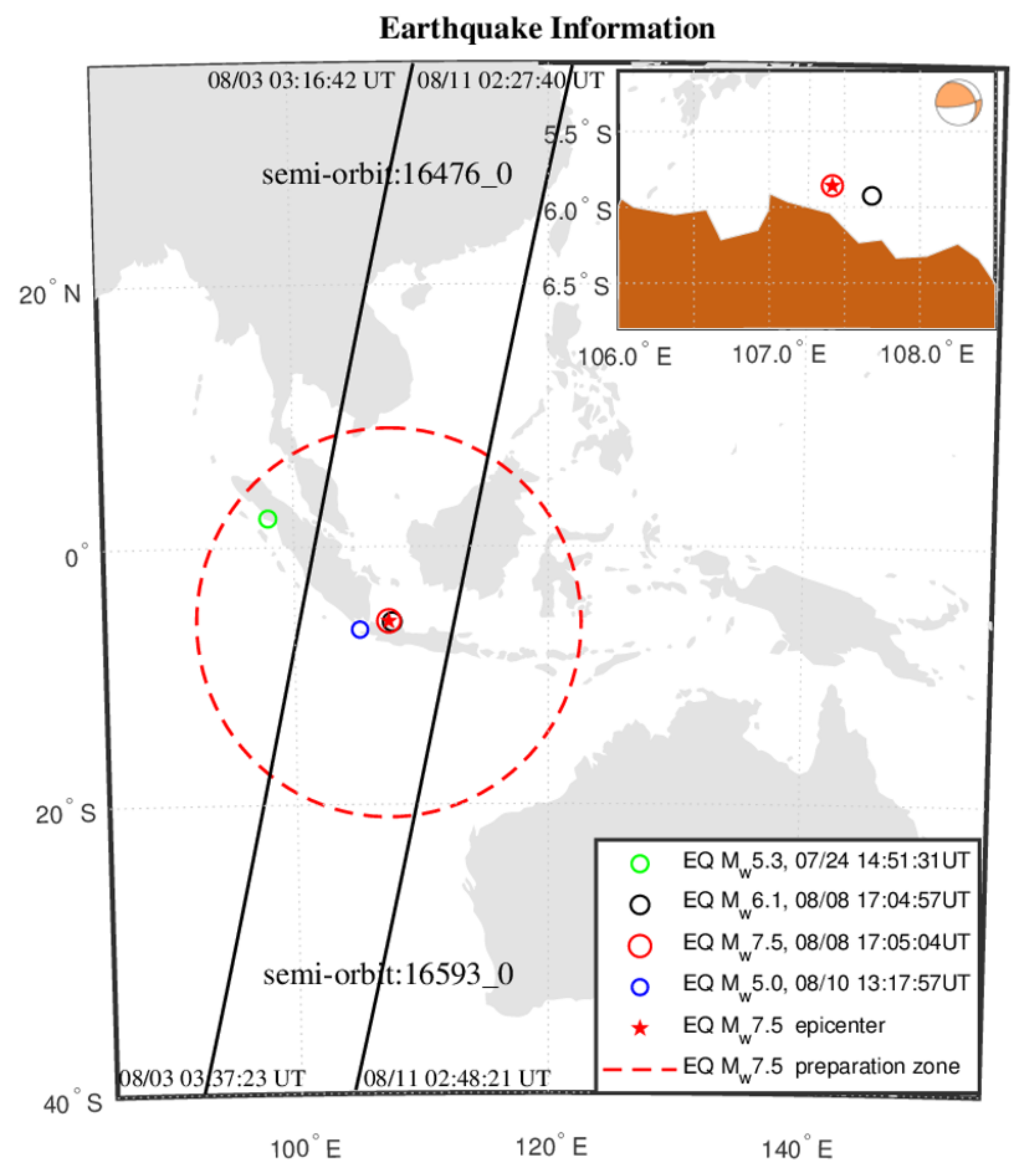
2. The 2007 M_w7.5 Jakarta–Java Earthquake

The deep hypocentral (280 km) main shock (oblique-reverse type) with magnitude $M_{w}7.5$ occurred in the offshore of Java Island ($5.86°\mathrm{S}, 107.42°\mathrm{E}$) at 17:05:04 UTC on 8 August 2007. Figure 1 displays this earthquake location and its preparation zone, which was estimated by Dobrovolsky formula as $\rho ={10}^{0.43·M}$, and here, M is the magnitude [55]. From 24 July to 13 August, there were another three $M_w\ge 5.0$ earthquakes around the main shock, as shown in Figure 1. In detail, the $M_{w}5.3$ earthquake occurred 15 days before the main shock, the $M_{w}6.1$ one occurred almost at the same time as the main shock and the $M_{w}5.0$ one was an aftershock on 10 August. This provides a relatively favorable condition for seismo-ionospheric analysis of the main shock. All earthquake data obtained from the National Earthquake Information Center (NEIC) ComCat database of the U.S. Geological Survey (https://earthquake.usgs.gov/earthquakes accessed on 29 March 2022).

3. Methodology and Observations

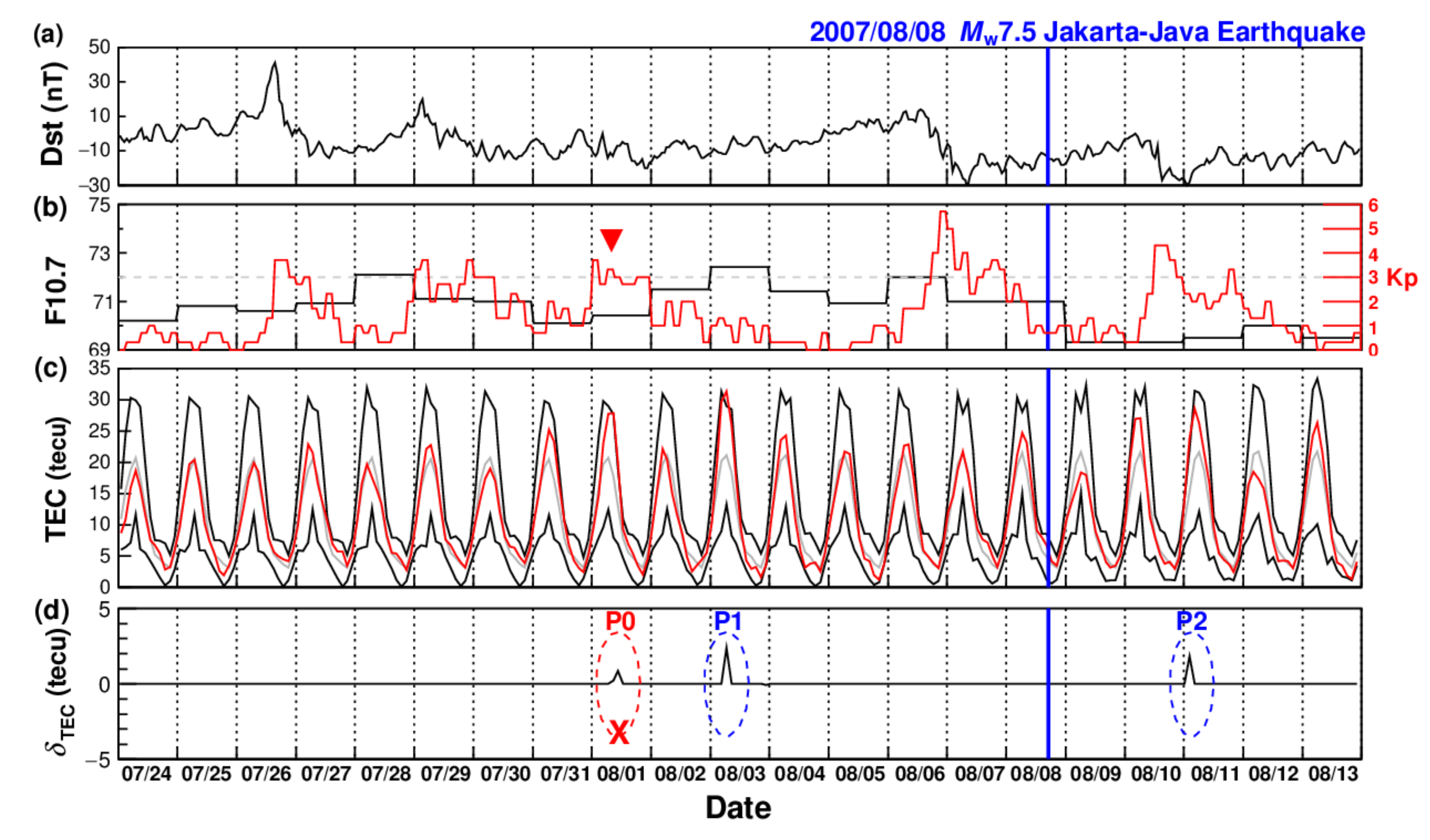
3.1. GIM TEC Temporal Anomalies

To detect the temporal anomalies over the epicenter of $M_{w}7.5$ Jakarta–Java earthquake, we examined GPS TEC to confirm the anomalies within 15 days before and 5 days after the main shock. TEC anomalies were detected by implementing confidence bounds of the median and associated interquartile ranges. Meanwhile, the bounds should be proportional to the earthquake magnitude. Here, a factor of 2.0 was set for the interquartile range value. The confidence bounds before and after the main shock are obtained from the median and interquartile range of reference data of 30 days before each observed day (i.e., 30-day running) using the below Equations (1) and (2) [7,9]:

$${\mathrm{TEC}}_{\mathrm{UB}}{ =\mathrm{MED}}_{30} + 2.0 · \mathrm{IQR}$$

(1)

$${\mathrm{TEC}}_{\mathrm{LB}}{ =\mathrm{MED}}_{30}- 2.0 · \mathrm{IQR}$$

(2)

where ${\mathrm{TEC}}_{\mathrm{UB}}$, ${\mathrm{TEC}}_{\mathrm{LB}}$, ${\mathrm{MED}}_{30}$ and $\mathrm{IQR}$ are the upper and lower bounds, median and interquartile range calculated by 30-day running TEC values, respectively.

In this paper, we computed the TEC values over the epicenter by using a linear interpolation of four data points nearest the epicenter. Deviations in TEC, namely, ${\mathsf{\delta }}_{\mathrm{TEC}}$, are defined in Equation (3) as the differences between observed TEC and confidence bounds:

$${\mathsf{\delta }}_{\mathrm{TEC} }=\left\{\begin{array}{c}{\mathrm{TEC}}_{\mathrm{observe} }-{ \mathrm{TEC}}_{\mathrm{UB}}\left({ > 0; \mathrm{when} \mathrm{TEC}}_{\mathrm{observe} }{> \mathrm{TEC}}_{\mathrm{UB}}\right)\\ {0(\mathrm{when} \mathrm{TEC}}_{\mathrm{observe}}{ =\mathrm{TEC}}_{\mathrm{UB}}{ \mathrm{or} \mathrm{TEC}}_{\mathrm{LB}})\\ {\mathrm{TEC}}_{\mathrm{observe} }-{ \mathrm{TEC}}_{\mathrm{LB}}{ ( < 0; \mathrm{when} \mathrm{TEC}}_{\mathrm{observe}}{ < \mathrm{TEC}}_{\mathrm{LB}})\end{array}\right.$$

(3)

To interpret the ionospheric anomalies over the epicenter, we examined GPS TEC to confirm the anomalies within 15 days before and 5 days after the main shock along with the confidence bounds, as shown in Figure 2c. Similarly, the ${\mathsf{\delta }}_{\mathrm{TEC}}$ values showed abnormal feature of daily TEC. According to Equation (3), three significant anomaly signals were automatically filtered out, namely, period P0–P2 illustrated in Figure 2d. It was worth noting that there are abnormal TEC enhancements during period P1 (06–08 UT on 3 August, exceeding the upper bound by +8.29%) and P2 (00–02 UT on 11 August, exceeding the upper bound by +8.27%). This was consistent with the previous results that the ionospheric TEC anomalies can occur a few days before and after strong earthquake [9,56,57,58,59,60]. However, the signal P0 (08–12 UT on 1 August, marked with red elliptic curve and cross in Figure 2d) was contaminated by magnetic storm activity and should be excluded if a stringent condition ($\mathrm{F}10.7 < 100 \mathrm{sfu}$, $\mathrm{Dst} > -30 \mathrm{nT}$ and $\mathrm{Kp} < 3.0$) was set for considering the potential impact of solar and geomagnetic activities. Furthermore, this affection for period P0 can also be confirmed by the results (for details please see the Supplementary Materials Figures S1 and S2) with following TEC-spatial-anomaly analysis in Section 3.2.

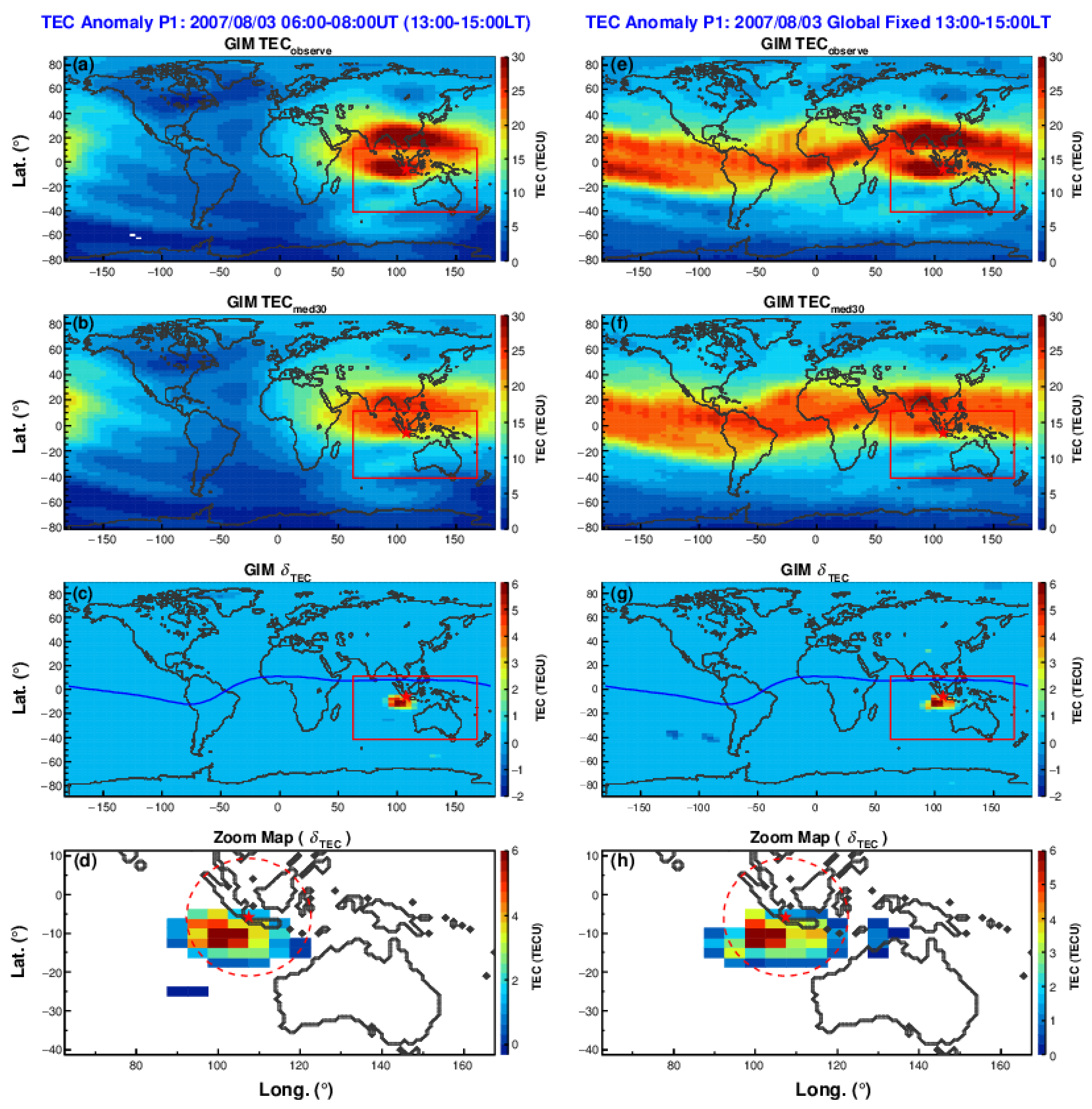
3.2. TEC Spatial Anomalies

In order to confirm the anomalous signals mentioned above, we conducted a spatial analysis to check if the GIM TECs simultaneously perturb over the epicenter. Figure 3 and Figure 4 show the GIM TECs LLT map for each anomalous period. The medians of the GIM TECs, as the background values, were computed with the data during the periods of day 1–30 before the observe ones. Then, the GIM extreme differences ($\left|{\mathsf{\delta }}_{\mathrm{TEC}}\right| > 0$) between the observed TEC and the associated 30-day running median one was obtained. As shown in Figure 3d and Figure 4d, the GIM TECs over the Jakarta–Java earthquake epicenter drastically enhanced up to ~+31.52% during period P1 and ~+13.85% during period P2, respectively. Furthermore, in order to exclude the local time and/or EIA (i.e., equatorial ionization anomaly) effects for the spatial analysis conducted above, the sequence of GIMs for the corresponding global fixed local times of anomalous periods are also examined. As shown in Figure 3h and Figure 4h, consistent with the above TEC enhancements at the universal time, the corresponding extreme enhancements (up to ~+31.52% during period P1 and ~+16.91% during period P2, respectively) during the global fixed local times are also mainly located around the epicenter. Meanwhile, these enhancements are also observed near to the magnetically conjugated region of the epicenter. It is worth noting that there is some regional background pollution of the deviations in TEC (${\mathsf{\delta }}_{\mathrm{TEC}}$) during period P2 (please see Figure 4c,g for details) probably due to geomagnetic activities ($\mathrm{Kp} > 3.0$) the day before, i.e., on 10 August.

Therefore, the spatial anomalies simultaneously and distinctly appear during the two anomalous periods around the epicenter of Jakarta–Java earthquake and its magnetically conjugated region.

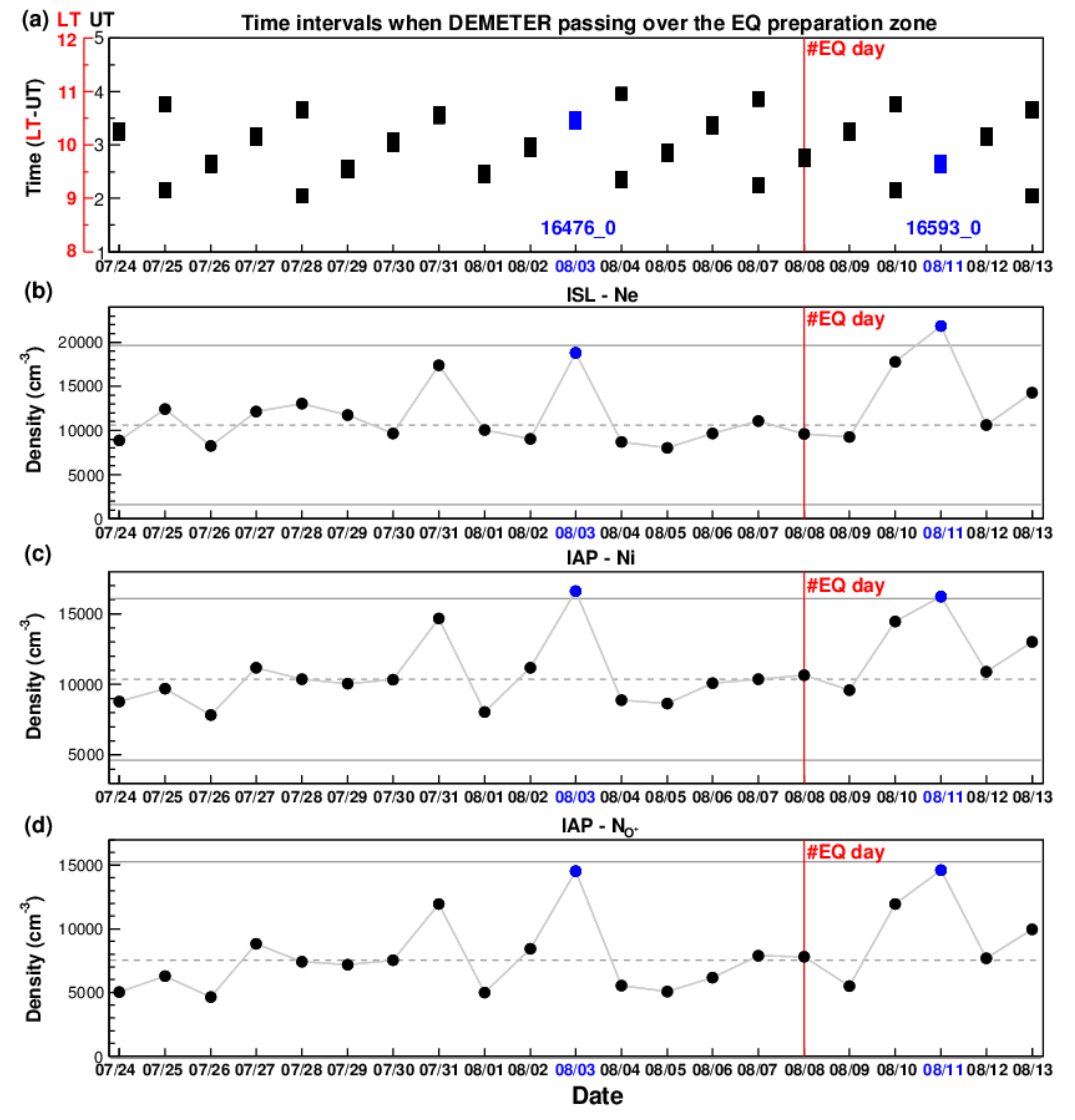
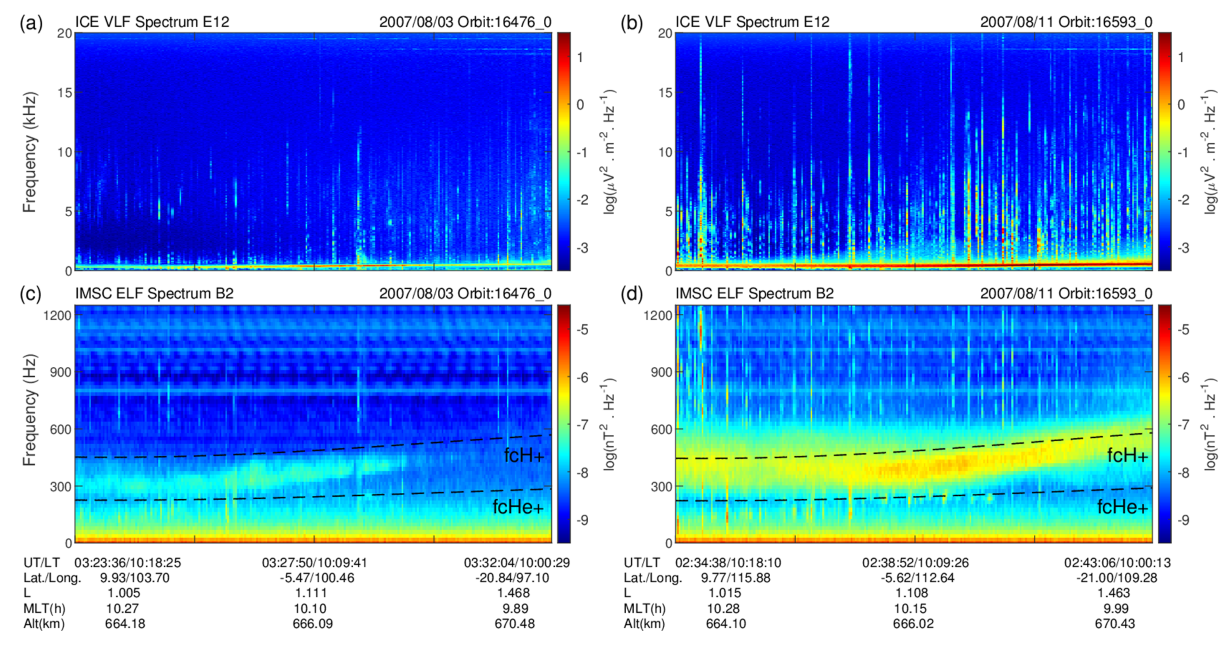
3.3. Ionospheric Plasma Anomalies

As described above, the GIM TEC anomalies extracted from GPS were analyzed from 15 days before to 5 days after the main shock. In order to further confirm ionospheric anomalies over the epicenter, a cross-validation analysis was also performed by using the data from the DEMETER satellite. Usually, the seismic-related anomalies observed by low-Earth orbit satellites deviate from the epicenter [61]. Similar to the methods described in Section 3.1, the undisturbed reference values (the medians, upper and lower confidence bounds) were calculated with the data recorded by instruments ISL and IAP onboard DEMETER above the earthquake preparation zone. Figure 5a illustrates the time intervals when the DEMETER satellite passed above the preparation zone in the daytime from 24 July to 13 August 2007. As shown in Figure 5b,c, both electron (Ne) and total ion densities (Ni) increase significantly and reach their maximum values of the study periods (+3.24% for Ni on 3 August, +10.03% for Ne and +0.95% for Ni on 11 August beyond the upper bound, respectively). In addition, the main ion component ${\mathrm{O}}^{+}$ density (${\mathrm{N}}_{{\mathrm{O}}^{+}}$) have a clear increasing trend (as seen in Figure 5d).

It should also be noted that the plasma parameters reach the extremum values during periods in the daytime (i.e., 10:18:25–10:00:29 LT on 3 August along the semi-orbit 16476_0 and 10:18:10–10:00:13 LT on 11 August along the semi-orbit 16593_0) when the satellite passed over the earthquake preparation zone in two down-going semi-orbits, as shown in Figure 1. This is also consistent with the fact that the GIM TEC enhancements were observed at the same daytime periods. However, the DEMETER satellite also passed through the earthquake preparation zone during the nighttime, but no similar variations were found.

4. Possible Natural and Artificial Electromagnetic Background

In order to identify the seismo-ionospheric anomalies, it is essential to assess the background due to natural non-seismic (such as atmospheric thunderstorms, volcanic eruptions and hurricane, etc.) or artificial (such as communications VLF transmitters and power line harmonic radiation, etc.) sources of electromagnetic emissions. Even so, solar wind can also affect the dynamics of the magnetosphere on a large scale, and the solar and geomagnetic conditions have been examined in Section 3.1.

4.1. Natural Non-Seismic Sources

Lightning is the main source of electromagnetic noise in the ionosphere, where it generates emissions from ELF up to VHF, although most of the energy is concentrated in the VLF band. Previous works have confirmed that powerful thunderstorm activities are able to perturb the ionosphere, including the enhancement of electron and ion (mainly ${\mathrm{O}}^{+}$) concentrations [62,63,64,65].

In this work, the power spectrum of the ELF magnetic field and VLF electric field were checked when the DEMETER was passing over the epicenter. It should be noted that data of magnetic field below ~200 Hz contain strong background noise due to the signals from payload DEMETER/IMSC being contaminated by parasitic signals or other sources of electromagnetic interference [66,67]. In Figure 6b, the spectrograms display vertical lines, which are the whistlers due to the thunderstorm activities. In addition, the DEMETER observations (Figure 6c,d) seem to have similar ELF spectra to low-altitude hiss waves that are commonly found in the ionosphere [68,69]. This electromagnetic whistler-mode hiss may leak out of the plasmasphere at higher altitude and then turn into low-altitude hiss in the ionosphere, which will play important roles for radiation belt loss and acceleration. For the event analyzed here, the ELF waves have weaker intensity due to being at dayside (about 10:00 LT). As the analysis duration is from July to August, it is summer close to the equator, and it is noteworthy that such significant plasma disturbances are not detected during other periods over the epicenter, as seen in Figure 5, even in the similar electromagnetic emission background. It can be illustrated, however, that along the semi-orbit 16593_0 where the electromagnetic background is relatively obvious but not very strong, the plasma disturbances due to electromagnetic factor cannot be completely excluded.

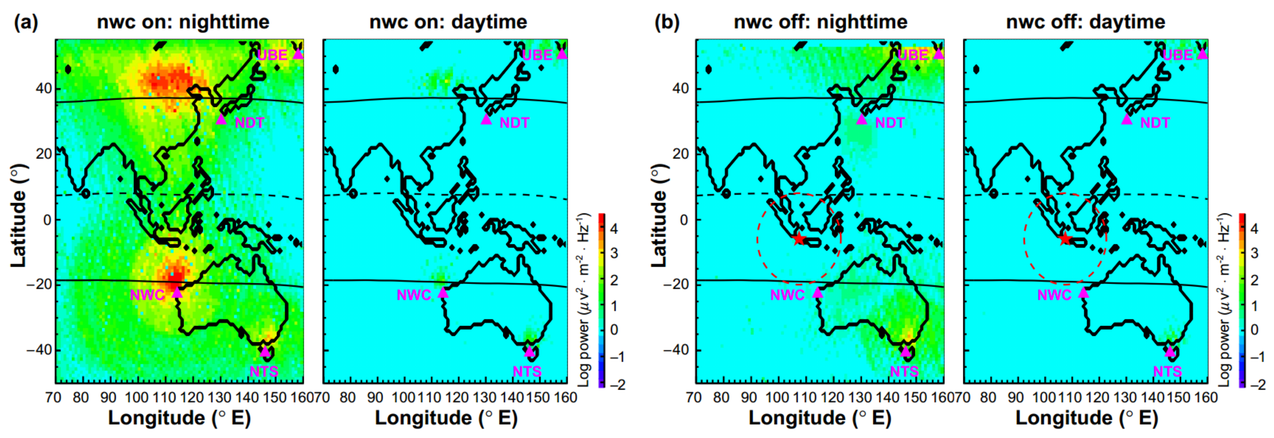
4.2. The Powerful Ground-Based VLF Transmitters

Many studies have shown that powerful ground-based communications from VLF transmitters around the tens of kHz frequency bands can trigger new waves, ionospheric heating, wave–particle interactions and particle precipitation via cyclotron resonance [70,71,72,73,74]. Because the power of the artificial signals can overwhelm the natural and faint emissions possibly associated to earthquakes, frequencies range around the band of the known VLF transmitters need to be considered in the analysis of seismo-associated disturbance.

Figure 7 displays the average power distribution measured by the ICE instrument aboard DEMETER during the nighttime and daytime, respectively. In the Asian sector (${70}^{°}\mathrm{E}$–${160}^{°}\mathrm{E}$), four main transmitters are long-running: UBE (at 16.20 kHz) and NDT (at 22.20 kHz) in the northern hemisphere and NWC (at 19.8 kHz) and NTS (at 18.60 kHz) in the southern hemisphere.

Table 1. The information of four VLF transmitters in the Asian sector.

No.	NAME	LAT.	LONG.	FREQ. (kHz)
1	UBE	52.90	158.55	16.20
2	NTS	−38.48	146.93	18.60
3	NWC	−21.82	114.17	19.80
4	NDT	32.08	130.83	22.20

provides the information of above four VLF transmitters. Among these VLF transmitters, the Naval Communication Station Harold E. Holt (“NWC”) in Western Australia is the most effective one. When NWC is on, its average power is about three orders of magnitude higher than the other three, and the distribution of VLF waves in the vicinity of Australia and in the conjugate hemisphere. However, the emission is significantly reduced when the NWC transmitter is off, i.e., from July 2007 to January 2008. Furthermore, compared to the nighttime, the daytime power is much lower because the stronger absorption in the ionosphere during the daytime (please see Figure 7b for details). In our case, the data analysis cycle (from 24 July to 13 August 2007) coincides with the off-time of NWC transmitter, and the two anomaly periods, i.e., P1 and P2, appear in the daytime. In view of this, we have reason to believe that the seismo-ionospheric anomaly here is minimally influenced by the known man-made VLF transmitters.

5. Discussion and Conclusions

In this work, the virtually simultaneous ionospheric TEC and plasma anomalies were detected over the epicenter during the 2007 $M_{w}7.5$ Jakarta–Java earthquake. Actually, there was another smaller $M_{w}6.1$ earthquake that occurred almost at the same time and immediately next to the epicenter of the main shock. It is thus difficult to distinguish exactly which one these disturbances are associated with, so here we consider all related anomalies as effects of the main shock. There are two clear abnormal signals, i.e., the enhancements during period P1 (on 3 August and day 5 before the main shock) and P2 (on 11 August and day 3 after the main shock), that were detected when we examined the temporal and spatial GIM TEC under stringent solar and geomagnetic conditions. This was consistent with the previous results that the ionospheric TEC anomalies can occur a few days before and after strong earthquake [9,56,57,58,59,60]. Taking into account the local time and/or EIA effects, the spatial enhancements also appear over the epicenter and consistent well with the above TEC enhancements at the universal time. Moreover, these enhancements are also observed simultaneously over, eastward to be precise, the epicenter and its magnetically conjugated region. In that sense, it may be explained by the mechanism of seismic–atmosphere–ionosphere–magnetosphere coupling, i.e., seismo-electromagnetic emissions can propagate as Alfven waves along the geomagnetic lines and resonantly interact with trapped electrons and eventually lead to electron precipitation [22,23] and shift eastward caused by plasma $\mathrm{E}\times \mathrm{B}$ drift [75]. Meanwhile, in order to confirm the above TEC anomalies, the plasma parameters are examined by using the DEMETER satellite, which has exactly two semi-orbits (i.e., 16476_0 on 3 August and 16593_0 on 11 August) passing through the earthquake preparation zone in the daytime. The significant increases both in electron (Ne) and total ion densities (Ni), reaching to the maximum values, are observed. In addition, the main ion component ${\mathrm{O}}^{+}$ density (${\mathrm{N}}_{{\mathrm{O}}^{+}}$) also shows a clear increasing trend. These plasma anomalies are also consistent with the TEC enhancements during the daytime. However, no similar disturbances were found during the nighttime, although the penetration of an anomalous electric field into the ionosphere in the nighttime will be more efficient than that in the daytime [76].

Nevertheless, it is still hard to completely confirm that the above ionospheric anomalies are related to the main shock, although the stringent solar and geomagnetic conditions have been adopted during the analysis process. Because solar wind can affect the dynamics of the magnetosphere on a large scale and last for a longer time, the contamination resulting from magnetic storm during period P0 on 1 August can therefore be distinctly observed, as shown in Figures S1 and S2c,g. As for the period P2, there is also some regional background pollution, which is probably due to geomagnetic activities ($\mathrm{Kp} > 3.0$) hours before in the deviations in TEC at high latitudes. At the same time, as we evaluated the electromagnetic emission background around period P2 from ELF to VLF, the whistlers due to the thunderstorm activities and local low-altitude hiss waves, both of which can play an important role for particles in the ionosphere and magnetosphere [64,65,68,69], were observed. It is worth realizing that this electromagnetic background is relatively weak and common in the ionosphere, and that is what happened during other periods of the entire study cycle (i.e., from 24 July to 13 August) when the DEMETER satellite passed above the preparation zone in the daytime. However, the potential impact during period P2 due to geomagnetic activities and the main natural non-seismic sources cannot be completely ignored and ruled out. In addition, there are evidences that enhancements in drift–loss cone fluxes in the inner radiation belt, i.e., electron bursts, coincide with the geographic and conjugate locations of the powerful VLF transmitter NWC [71,77]. Fortunately, the study cycle of this work is coinciding with the off-time of the NWC transmitter, and the anomaly periods are minimally influenced by these man-made VLF transmitters. Anyhow, the difficulties of this work should be recognized and approached with caution in detecting seismo-ionospheric anomalies.

Although the possible earthquake-related disturbances observed in space have been reported in many previous studies, the physical mechanism for coupling the lithosphere with lower and upper layers of the atmosphere up to the ionosphere is still open and disputed. To explain these abnormal disturbances occurring before earthquakes, some coupling mechanisms and theoretical models have been suggested and developed, such as low frequency electromagnetic radiation [14,78], quasi-static electric fields and currents [79,80] and waves of the neutral atmosphere [81,82]. Even so, due to the variability or uncertainty in the temporal and spatial scales of the seismic ionospheric fluctuations, it is still difficult to interpret them by only one mechanism. On the one hand, the anomalous vertical electric field near the Earth’s surface above the seismogenic zone can penetrate into the ionosphere effectively and eventually lead to ionospheric irregularities [79,80]. Pulinets et al. [80] assumed that the increased scale of the disturbance zone for deep-focus (60–300 km) earthquakes would generate a vertical electrical disturbance up to 200–250 km in diameter near the Earth’s surface, i.e., large enough to create a significant disturbance in the ionosphere. On the other hand, considering the focal depth (280 km) of a large undersea earthquake and its energy loss transmitted to the seafloor, atmospheric waves seem to be another potential or more efficient channel for energy transport into the ionosphere, although no wave-like features were found in our results. Recently, Inchin et al. [26,27] have successfully reproduced the ionospheric responses to seismically induced atmospheric infrasonic/acoustic and gravity waves, which can excite at water–air interfaces and propagate into the upper layers of the atmosphere and generate fluctuations in densities, temperatures and ionospheric plasma. In addition, possible gases (including radioactive radon, CO₂ and CH₄, etc.) and aerosols released during the earthquake (both inland and undersea cases) preparation phase can explain the model of atmospheric thermal anomalies well, which could generate atmospheric oscillations and then trigger acoustic gravity waves [83,84,85,86,87]. For example, Molchanov et al. [86] suggested a complete model of atmospheric gravity waves (AGW), in which an upward energy flux of AGW induced by the gas–water release from the seismic region can penetrate into the ionosphere to modify the ionospheric plasma background and form a turbulence in scales of ~1 to 3 km. Up to now, the atmospheric waves are thought to play a key role in the LAI coupling process, and further support to this hypothesis should be provided in future. Fortunately, the high-density geophysical arrays for monitoring vibrations and perturbations in the LAI (also called the MVP–LAI system) were established in China in 2021 [88]. It will provide an excellent opportunity for monitoring vibrations and perturbations in the vertical direction (including the atmospheric waves) and promote the understanding the physical mechanism of LAI coupling.

In conclusion, the significant TEC temporal and spatial anomalies were detected during periods P1 and P2 over the epicenter of the 2007 $M_{w}7.5$ Jakarta–Java earthquake, and they coincide well with the striking plasma anomalies in the ionosphere observed in situ by the LEO satellite. The localization and synchronization of the disturbances during the earthquake suggest that these ionospheric anomalies are highly related to this great deep-focus undersea earthquake. Despite the electromagnetic background, mainly due to geomagnetic and thunderstorm activities and local low-altitude hiss, is a bit complicated during period P2. Nevertheless, the coupling process is still not fully understood in great detail and needs further statistical investigation, and deep-focus undersea seismic events especially need to be treated more carefully and discreetly in the future.

References

1. Jones, L.; Molnar, P. Frequency of foreshocks. Nature 1976, 262, 677–679. [Google Scholar] [CrossRef]
2. Sornette, A.; Sornette, D. Self-organized criticality and earthquakes. Europhys. Lett. 1989, 9, 197–202. [Google Scholar] [CrossRef]
3. De Santis, A. Geosystemics, Entropy and Criticality of Earthquakes: A Vision of Our Planet and a Key of Access. In Nonlinear Phenomena in Complex Systems: From Nano to Macro Scale; Springer: Berlin/Heidelberg, Germany, 2013; pp. 3–20. [Google Scholar]
4. De Santis, A.; De Franceschi, G.; Spogli, L.; Perrone, L.; Alfonsi, L.; Qamili, E.; Cianchini, G.; Di Giovambattista, R.; Salvi, S.; Filippi, E.; et al. Geospace perturbations induced by the Earth: The state of the art and future trends. Phys. Chem. Earth 2015, 85, 17–33. [Google Scholar] [CrossRef]
5. Picozza, P.; Conti, L.; Sotgiu, A. Looking for Earthquake Precursors from Space: A Critical Review. Front. Earth Sci. 2021, 9, 578. [Google Scholar] [CrossRef]
6. Conti, L.; Picozza, P.; Sotgiu, A. A Critical Review of Ground Based Observations of Earthquake Precursors. Front. Earth Sci. 2021, 9, 676766. [Google Scholar] [CrossRef]
7. Liu, J.Y.; Chuo, Y.J.; Shan, S.J.; Tsai, Y.B.; Chen, Y.I.; Pulinets, S.A.; Yu, S.B. Pre-earthquake ionospheric anomalies registered by continuous GPS TEC measurements. Ann. Geophys. Ger. 2004, 22, 1585–1593. [Google Scholar] [CrossRef]
8. Liu, J.Y.; Chen, C.H.; Chen, V.I.; Yang, W.H.; Oyama, K.I.; Kuo, K.W. A statistical study of ionospheric earthquake precursors monitored by using equatorial ionization anomaly of GPS TEC in Taiwan during 2001–2007. J. Asian Earth Sci. 2010, 39, 76–80. [Google Scholar] [CrossRef]
9. Akhoondzadeh, M.; Parrot, M.; Saradjian, M.R. Electron and ion density variations before strong earthquakes (M > 6.0) using DEMETER and GPS data. Nat. Hazard Earth Sys. 2010, 10, 7–18. [Google Scholar] [CrossRef]
10. Tao, D.; Cao, J.; Battiston, R.; Li, L.; Ma, Y.; Liu, W.; Zhima, Z.; Wang, L.; Dunlop, M.W. Seismo-ionospheric anomalies in ionospheric TEC and plasma density before the 17 July 2006 M7.7 south of Java earthquake. Ann. Geophys. Ger. 2017, 35, 589–598. [Google Scholar] [CrossRef]
11. Kuo, C.L.; Huba, J.D.; Joyce, G.; Lee, L.C. Ionosphere plasma bubbles and density variations induced by pre-earthquake rock currents and associated surface charges. J. Geophys. Res. Space 2011, 116, A10317. [Google Scholar] [CrossRef]
12. Ma, W.; Zhang, X.; Jun, L.; Qi, Y.; Bo, Z.; Chong, Y.; Kang, C.; Xian, L. Influences of multiple layers of air temperature differences on tidal forces and tectonic stress before, during and after the Jiujiang earthquake. Remote Sens. Environ. 2018, 210, 159–165. [Google Scholar] [CrossRef]
13. Zhang, X.; Wang, Y.; Boudjada, M.; Liu, J.; Magnes, W.; Zhou, Y.; Du, X. Multi-Experiment Observations of Ionospheric Disturbances as Precursory Effects of the Indonesian Ms6.9 Earthquake on August 05, 2018. Remote Sens. 2020, 12, 4050. [Google Scholar] [CrossRef]
14. Parrot, M. Statistical study of ELF/VLF emissions recorded by a low-altitude satellite during seismic events. J. Geophys. Res. Space Phys. 1994, 99, 23339–23347. [Google Scholar] [CrossRef]
15. Nemec, F.; Santolik, O.; Parrot, M.; Berthelier, J.J. Spacecraft observations of electromagnetic perturbations connected with seismic activity. Geophys. Res. Lett. 2008, 35, L05109. [Google Scholar] [CrossRef]
16. Nemec, F.; Santolik, O.; Parrot, M. Decrease of intensity of ELF/VLF waves observed in the upper ionosphere close to earthquakes: A statistical study. J. Geophys. Res. Space 2009, 114, A04303. [Google Scholar] [CrossRef]
17. Pisa, D.; Nemec, F.; Santolik, O.; Parrot, M.; Rycroft, M. Additional attenuation of natural VLF electromagnetic waves observed by the DEMETER spacecraft resulting from preseismic activity. J. Geophys. Res. Space 2013, 118, 5286–5295. [Google Scholar] [CrossRef]
18. Ouzounov, D.; Freund, F. Mid-infrared emission prior to strong earthquakes analyzed by remote sensing data. Adv. Space Res. 2004, 33, 268–273. [Google Scholar] [CrossRef]
19. Tramutoli, V.; Cuomo, V.; Filizzola, C.; Pergola, N.; Pietrapertosa, C. Assessing the potential of thermal infrared satellite surveys for monitoring seismically active areas: The case of Kocaell (Izmit) earthquake, August 17, 1999. Remote Sens. Environ. 2005, 96, 409–426. [Google Scholar] [CrossRef]
20. Ouzounov, D.; Liu, D.; Kang, C.; Cervone, G.; Kafatos, M.; Taylor, P. Outgoing long wave radiation variability from IR satellite data prior to major earthquakes. Tectonophysics 2007, 431, 211–220. [Google Scholar] [CrossRef]
21. Lu, X.; Meng, Q.Y.; Gu, X.F.; Zhang, X.D.; Xie, T.; Geng, F. Thermal infrared anomalies associated with multi-year earthquakes in the Tibet region based on China’s FY-2E satellite data. Adv. Space Res. 2016, 58, 989–1001. [Google Scholar] [CrossRef]
22. Aleksandrin, S.Y.; Galper, A.M.; Grishantzeva, L.A.; Koldashov, S.V.; Maslennikov, L.V.; Murashov, A.M.; Picozza, P.; Sgrigna, V.; Voronov, S.A. High-energy charged particle bursts in the near-Earth space as earthquake precursors. Ann. Geophys. Ger. 2003, 21, 597–602. [Google Scholar] [CrossRef]
23. Sgrigna, V.; Carota, L.; Conti, L.; Corsi, M.; Galper, A.M.; Koldashov, S.V.; Murashov, A.M.; Picozza, P.; Scrimaglio, R.; Stagni, L. Correlations between earthquakes and anomalous particle bursts from SAMPEX/PET satellite observations. J. Atmos. Sol. Terr. Phys. 2005, 67, 1448–1462. [Google Scholar] [CrossRef]
24. Battiston, R.; Vitale, V. First evidence for correlations between electron fluxes measured by NOAA-POES satellites and large seismic events. Nucl. Phys. B Proc. Suppl. 2013, 243, 249–257. [Google Scholar] [CrossRef]
25. Kuo, C.L.; Lee, L.C.; Huba, J.D. An improved coupling model for the lithosphere-atmosphere-ionosphere system. J. Geophys. Res. Space 2014, 119, 3189–3205. [Google Scholar] [CrossRef]
26. Inchin, P.A.; Snively, J.B.; Zettergren, M.D.; Komjathy, A.; Verkhoglyadova, O.P.; Ram, S.T. Modeling of Ionospheric Responses to Atmospheric Acoustic and Gravity Waves Driven by the 2015 Nepal M(w)7.8 Gorkha Earthquake. J. Geophys. Res. Space 2020, 125, e2019JA027200. [Google Scholar] [CrossRef]
27. Inchin, P.A.; Snively, J.B.; Kaneko, Y.; Zettergren, M.D.; Komjathy, A. Inferring the Evolution of a Large Earthquake from Its Acoustic Impacts on the Ionosphere. Agu Adv. 2021, 2, e2020AV000260. [Google Scholar] [CrossRef]
28. Xiong, P.; Long, C.; Zhou, H.; Battiston, R.; Zhang, X.; Shen, X. Identification of Electromagnetic Pre-Earthquake Perturbations from the DEMETER Data by Machine Learning. Remote Sens. 2020, 12, 3643. [Google Scholar] [CrossRef]
29. Xiong, P.; Tong, L.; Zhang, K.; Shen, X.; Battiston, R.; Ouzounov, D.; Iuppa, R.; Crookes, D.; Long, C.; Zhou, H. Towards advancing the earthquake forecasting by machine learning of satellite data. Sci. Total Environ. 2021, 771, 145256. [Google Scholar] [CrossRef]
30. Heki, K.; Otsuka, Y.; Choosakul, N.; Hemmakorn, N.; Komolmis, T.; Maruyama, T. Detection of ruptures of Andaman fault segments in the 2004 great Sumatra earthquake with coseismic ionospheric disturbances. J. Geophys. Res. Solid Earth 2006, 111, B09313. [Google Scholar] [CrossRef]
31. Liu, J.Y.; Tsai, H.F.; Lin, C.H.; Kamogawa, M.; Chen, Y.I.; Lin, C.H.; Huang, B.S.; Yu, S.B.; Yeh, Y.H. Coseismic ionospheric disturbances triggered by the Chi-Chi earthquake. J. Geophys. Res. Space 2010, 115, A08303. [Google Scholar] [CrossRef]
32. Song, Q.; Ding, F.; Yu, T.; Wan, W.; Ning, B.; Liu, L.; Zhao, B. GPS detection of the coseismic ionospheric disturbances following the 12 May 2008 M7.9 Wenchuan earthquake in China. Sci. China Earth Sci. 2015, 58, 151–158. [Google Scholar] [CrossRef]
33. Gao, Y.; Harris, J.M.; Wen, J.; Huang, Y.; Twardzik, C.; Chen, X.; Hu, H. Modeling of the coseismic electromagnetic fields observed during the 2004 M-w 6.0 Parkfield earthquake. Geophys. Res. Lett. 2016, 43, 620–627. [Google Scholar] [CrossRef]
34. Ram, S.T.; Sunil, P.S.; Kumar, M.R.; Su, S.Y.; Tsai, L.C.; Liu, C.H. Coseismic Traveling Ionospheric Disturbances during the M-w 7.8 Gorkha, Nepal, Earthquake on 25 April 2015 from Ground and Spaceborne Observations. J. Geophys. Res. Space 2017, 122, 10669–10685. [Google Scholar] [CrossRef]
35. Liu, H.; Zhang, K.; Imtiaz, N.; Song, Q.; Zhang, Y. Relating Far-Field Coseismic Ionospheric Disturbances to Geological Structures. J. Geophys. Res. Space 2021, 126, e2021JA029209. [Google Scholar] [CrossRef]
36. Pustovetov, V.P.; Malyshev, A.B. Space–time correlation of earthquakes and high-energy particle flux variations in the inner radiation belt. Cosm. Res. 1993, 31, 84–90. [Google Scholar]
37. Le, H.; Liu, J.Y.; Liu, L. A statistical analysis of ionospheric anomalies before 736 M6.0+earthquakes during 2002–2010. J. Geophys. Res. Space 2011, 116, A02303. [Google Scholar] [CrossRef]
38. Xia, C.; Yang, S.; Xu, G.; Zhao, B.; Yu, T. Ionospheric Anomalies Observed by GPS TEC Prior to the Qinghai-Tibet Region Earthquakes. Terr. Atmos. Ocean Sci. 2011, 22, 177–185. [Google Scholar] [CrossRef]
39. Harper, W.R. The generation of static charge. Adv. Phys. 1957, 6, 365–417. [Google Scholar] [CrossRef]
40. Blanchard, D.C. The electrification of the atmosphere by particles from bubbles in the sea. Prog. Oceanogr. 1963, 1, 73–202. [Google Scholar] [CrossRef]
41. King, C.Y. Gas geochemistry applied to earthquake prediction: An overview. J. Geophys. Res. Solid Earth 1986, 91, 12269–12281. [Google Scholar] [CrossRef]
42. Zavarsky, A.; Booge, D.; Fiehn, A.; Kruger, K.; Atlas, E.; Marandino, C. The Influence of Air-Sea Fluxes on Atmospheric Aerosols During the Summer Monsoon Over the Tropical Indian Ocean. Geophys. Res. Lett. 2018, 45, 418–426. [Google Scholar] [CrossRef]
43. Revell, L.E.; Kremser, S.; Hartery, S.; Harvey, M.; Mulcahy, J.P.; Williams, J.; Morgenstern, O.; McDonald, A.J.; Varma, V.; Bird, L.; et al. The sensitivity of Southern Ocean aerosols and cloud microphysics to sea spray and sulfate aerosol production in the HadGEM3-GA7.1 chemistry-climate model. Atmos. Chem. Phys. 2019, 19, 15447–15466. [Google Scholar] [CrossRef]
44. Sorokin, V.M.; Chmyrev, V.M.; Hayakawa, M. A Review on Electrodynamic Influence of Atmospheric Processes to the Ionosphere. Open J. Earthq. Res. 2020, 9, 113–141. [Google Scholar] [CrossRef]
45. Blanc, E. Observations in the upper atmosphere of infrasonic waves from natural or artificial sources-A summary. Ann. Geophys. Ger. 1985, 3, 673–687. [Google Scholar]
46. Kaladze, T.D.; Pokhotelov, O.A.; Shah, H.A.; Khan, M.I.; Stenflo, L. Acoustic-gravity waves in the Earth’s ionosphere. J. Atmos. Sol. Terr. Phys. 2008, 70, 1607–1616. [Google Scholar] [CrossRef]
47. Godin, O.A. Acoustic-gravity waves in atmospheric and oceanic waveguides. J. Acoust. Soc. Am. 2012, 132, 657–669. [Google Scholar] [CrossRef]
48. Zettergren, M.D.; Snively, J.B. Ionospheric response to infrasonic-acoustic waves generated by natural hazard events. J. Geophys. Res. Space 2015, 120, 8002–8024. [Google Scholar] [CrossRef]
49. Kadri, U. Tsunami mitigation by resonant triad interaction with acoustic-gravity waves. Heliyon 2017, 3, e00234. [Google Scholar] [CrossRef]
50. Yang, S.-S.; Asano, T.; Hayakawa, M. Abnormal Gravity Wave Activity in the Stratosphere Prior to the 2016 Kumamoto Earthquakes. J. Geophys. Res. Space 2019, 124, 1410–1425. [Google Scholar] [CrossRef]
51. Kakinami, Y.; Kamogawa, M.; Tanioka, Y.; Watanabe, S.; Gusman, A.R.; Liu, J.-Y.; Watanabe, Y.; Mogi, T. Tsunamigenic ionospheric hole. Geophys. Res. Lett. 2012, 39, L00G27. [Google Scholar] [CrossRef]
52. Song, R.; Hattori, K.; Zhang, X.; Sanaka, S. Seismic-ionospheric effects prior to four earthquakes in Indonesia detected by the China seismo-electromagnetic satellite. J. Atmos. Sol. Terr. Phys. 2020, 205, 105291. [Google Scholar] [CrossRef]
53. Roma-Dollase, D.; Hernandez-Pajares, M.; Krankowski, A.; Kotulak, K.; Ghoddousi-Fard, R.; Yuan, Y.; Li, Z.; Zhang, H.; Shi, C.; Wang, C.; et al. Consistency of seven different GNSS global ionospheric mapping techniques during one solar cycle. J. Geod. 2018, 92, 691–706. [Google Scholar] [CrossRef]
54. Parrot, M.; Benoist, D.; Berthelier, J.J.; Blecki, J.; Chapuis, Y.; Colin, F.; Elie, F.; Fergeau, P.; Lagoutte, D.; Lefeuvre, F.; et al. The magnetic field experiment IMSC and its data processing onboard DEMETER: Scientific objectives, description and first results. Planet Space Sci. 2006, 54, 441–455. [Google Scholar] [CrossRef]
55. Dobrovolsky, I.P.; Zubkov, S.I.; Miachkin, V.I. Estimation of the size of earthquake preparation zones. Pure Appl. Geophys. 1979, 117, 1025–1044. [Google Scholar] [CrossRef]
56. Pulinets, S.A.; Legen’ka, A.D.; Gaivoronskaya, T.V.; Depuev, V.K. Main phenomenological features of ionospheric precursors of strong earthquakes. J. Atmos. Sol. Terr. Phys. 2003, 65, 1337–1347. [Google Scholar] [CrossRef]
57. Pulinets, S.; Davidenko, D. Ionospheric precursors of earthquakes and Global Electric Circuit. Adv. Space Res. 2014, 53, 709–723. [Google Scholar] [CrossRef]
58. Pulinets, S.A.; Ouzounov, D.P.; Karelin, A.V.; Davidenko, D.V. Physical bases of the generation of short-term earthquake precursors: A complex model of ionization-induced geophysical processes in the lithosphere-atmosphere-ionosphere-magnetosphere system. Geomagn. Aeron. 2015, 55, 521–538. [Google Scholar] [CrossRef]
59. Liu, J.Y.; Chen, Y.I.; Chen, C.H.; Hattori, K. Temporal and spatial precursors in the ionospheric global positioning system (GPS) total electron content observed before the 26 December 2004 M9.3 Sumatra-Andaman Earthquake. J. Geophys. Res. Space 2010, 115, A09312. [Google Scholar] [CrossRef]
60. Liu, J.; Zhang, X.; Novikov, V.; Shen, X. Variations of ionospheric plasma at different altitudes before the 2005 Sumatra Indonesia M-s 7.2 earthquake. J. Geophys. Res. Space 2016, 121, 9179–9187. [Google Scholar] [CrossRef]
61. Zhima, Z.; Cao, J.; Liu, W.; Fu, H.; Wang, T.; Zhang, X.; Shen, X. Storm time evolution of ELF/VLF waves observed by DEMETER satellite. J. Geophys. Res. Space 2014, 119, 2612–2622. [Google Scholar] [CrossRef]
62. Voss, H.D.; Imhof, W.L.; Walt, M.; Mobilia, J.; Gaines, E.E.; Reagan, J.B.; Inan, U.S.; Helliwell, R.A.; Carpenter, D.L.; Katsufrakis, J.P.; et al. Lightning-induced electron precipitation. Nature 1984, 312, 740–742. [Google Scholar] [CrossRef]
63. Rodger, C.J.; Cho, M.G.; Clilverd, M.A.; Rycroft, M.J. Lower ionospheric modification by lightning-EMP: Simulation of the night ionosphere over the United States. Geophys. Res. Lett. 2001, 28, 199–202. [Google Scholar] [CrossRef]
64. Parrot, M.; Berthelier, J.J.; Lebreton, J.P.; Treumann, R.; Rauch, J.L. DEMETER observations of EM emissions related to thunderstorms. Space Sci. Rev. 2008, 137, 511–519. [Google Scholar] [CrossRef]
65. Parrot, M.; Sauvaud, J.A.; Soula, S.; Pincon, J.L.; van der Velde, O. Ionospheric density perturbations recorded by DEMETER above intense thunderstorms. J. Geophys. Res. Space 2013, 118, 5169–5176. [Google Scholar] [CrossRef]
66. Cao, J.; Yang, J.; Yuan, S.; Shen, X.; Liu, Y.; Yan, C.; Li, W.; Chen, T. In-flight observations of electromagnetic interferences emitted by satellite. Sci. China Ser. E Technol. Sci. 2009, 52, 2112–2118. [Google Scholar] [CrossRef]
67. Zhima, Z.; Shen, X.; Zhang, X.; Cao, J.; Huang, J.; Ouyang, X.; Jing, L.; Lu, B. Possible Ionospheric Electromagnetic Perturbations Induced by the Ms7.1 Yushu Earthquake. Earth Moon Planets 2012, 108, 231–241. [Google Scholar] [CrossRef]
68. Chen, L.; Santolik, O.; Hajos, M.; Zheng, L.; Zhima, Z.; Heelis, R.; Hanzelka, M.; Horne, R.B.; Parrot, M. Source of the low-altitude hiss in the ionosphere. Geophys. Res. Lett. 2017, 44, 2060–2069. [Google Scholar] [CrossRef]
69. Chen, L.; Pfaff, R.; Heelis, R.; Boardsen, S.; Xia, Z. Ion Cyclotron Resonant Absorption Lines in ELF Hiss Power Spectral Density in the Low-Latitude Ionosphere. Geophys. Res. Lett. 2020, 47, e2019GL086315. [Google Scholar] [CrossRef]
70. Sauvaud, J.A.; Maggiolo, R.; Jacquey, C.; Parrot, M.; Berthelier, J.J.; Gamble, R.J.; Rodger, C.J. Radiation belt electron precipitation due to VLF transmitters: Satellite observations. Geophys. Res. Lett. 2008, 35, L09101. [Google Scholar] [CrossRef]
71. Gamble, R.J.; Rodger, C.J.; Clilverd, M.A.; Sauvaud, J.-A.; Thomson, N.R.; Stewart, S.L.; McCormick, R.J.; Parrot, M.; Berthelier, J.-J. Radiation belt electron precipitation by man-made VLF transmissions. J. Geophys. Res. Space 2008, 113, A10211. [Google Scholar] [CrossRef]
72. Li, X.; Ma, Y.; Wang, P.; Wang, H.; Lu, H.; Zhang, X.; Huang, J.; Shi, F.; Yu, X.; Xu, Y.; et al. Study of the North West Cape electron belts observed by DEMETER satellite. J. Geophys. Res. Space Phys. 2012, 117, A04201. [Google Scholar] [CrossRef]
73. Selesnick, R.S.; Albert, J.M.; Starks, M.J. Influence of a ground-based VLF radio transmitter on the inner electron radiation belt. J. Geophys. Res. Space Phys. 2013, 118, 628–635. [Google Scholar] [CrossRef]
74. Sauvaud, J.A.; Walt, M.; Delcourt, D.; Benoist, C.; Penou, E.; Chen, Y.; Russell, C.T. Inner radiation belt particle acceleration and energy structuring by drift resonance with ULF waves during geomagnetic storms. J. Geophys. Res. Space 2013, 118, 1723–1736. [Google Scholar] [CrossRef]
75. Liu, J.Y.; Chen, Y.I.; Chen, C.H.; Liu, C.Y.; Chen, C.Y.; Nishihashi, M.; Li, J.Z.; Xia, Y.Q.; Oyama, K.I.; Hattori, K.; et al. Seismoionospheric GPS total electron content anomalies observed before the 12 May 2008 M(w)7.9 Wenchuan earthquake. J. Geophys. Res. Space 2009, 114, A04320. [Google Scholar] [CrossRef]
76. Pulinets, S. Ionospheric precursors of earthquakes; Recent advances in theory and practical applications. Terr. Atmos. Ocean Sci. 2004, 15, 413–435. [Google Scholar] [CrossRef]
77. Sidiropoulos, N.F.; Anagnostopoulos, G.; Rigas, V. Comparative study on earthquake and ground based transmitter induced radiation belt electron precipitation at middle latitudes. Nat. Hazard Earth Syst. 2011, 11, 1901–1913. [Google Scholar] [CrossRef]
78. Dudkin, F.; Korepanov, V.; Dudkin, D.; Pilipenko, V.; Pronenko, V.; Klimov, S. Electric field of the power terrestrial sources observed by microsatellite Chibis-M in the Earth’s ionosphere in frequency range 1-60 Hz. Geophys. Res. Lett. 2015, 42, 5686–5693. [Google Scholar] [CrossRef]
79. Pulinets, S.A.; Boyarchuk, K.A.; Hegai, V.V.; Kim, V.P.; Lomonosov, A.M. Quasielectrostatic model of atmosphere-thermosphere-ionosphere coupling. Adv. Space Res. 2000, 26, 1209–1218. [Google Scholar] [CrossRef]
80. Pulinets, S.A.; Boyarchuk, K.A.; Lomonosov, A.M.; Khegai, V.V.; Lyu, I.Y. Ionospheric precursors to earthquakes: A preliminary analysis of the foF2 critical frequencies at Chung-Li ground-based station for vertical sounding of the ionosphere (Taiwan Island). Geomagn. Aeron. 2002, 42, 508–513. [Google Scholar]
81. Korepanov, V.; Hayakawa, M.; Yampolski, Y.; Lizunov, G. AGW as a seismo-ionospheric coupling responsible agent. Phys. Chem. Earth 2009, 34, 485–495. [Google Scholar] [CrossRef]
82. Hayakawa, M.; Asano, T.; Rozhnoi, A.; Solovieva, M. Very-Low and Low-Frequency Sounding of Ionospheric Perturbations and Possible Association with Earthquakes. In Pre-Earthquake Process: A Multidisciplinary Approach to Earthquake Prediction Studies; Ouzounov, D., Pulinets, S., Hattori, K., Taylor, P., Eds.; AGU: Washington, DC, USA, 2018; pp. 277–304. [Google Scholar]
83. Garavaglia, M.; Dal Moro, G.; Zadro, M. Radon and tilt measurements in a seismic area: Temperature effects. Phys. Chem. Earth Part A-Solid Earth Geod. 2000, 25, 233–237. [Google Scholar] [CrossRef]
84. Silva, A.A.; Claro, L.H. Surface air radon progeny at Sao Jose dos Campos, Brazil. Atmos. Environ. 2005, 39, 4619–4625. [Google Scholar] [CrossRef]
85. Pulinets, S.A.; Ouzounov, D.; Karelin, A.V.; Boyarchuk, K.A.; Pokhmelnykh, L.A. The physical nature of thermal anomalies observed before strong earthquakes. Phys. Chem. Earth 2006, 31, 143–153. [Google Scholar] [CrossRef]
86. Molchanov, O.; Rozhnoi, A.; Solovieva, M.; Akentieva, O.; Berthelier, J.J.; Parrot, M.; Lefeuvre, F.; Biagi, P.F.; Castellana, L.; Hayakawa, M. Global diagnostics of the ionospheric perturbations related to the seismic activity using the VLF radio signals collected on the DEMETER satellite. Nat. Hazard Earth Syst. 2006, 6, 745–753. [Google Scholar] [CrossRef]
87. Pulinets, S.; Ouzounov, D. Lithosphere-Atmosphere-Ionosphere Coupling (LAIC) model—An unified concept for earthquake precursors validation. J. Asian Earth Sci. 2011, 41, 371–382. [Google Scholar] [CrossRef]
88. Chen, C.-H.; Sun, Y.-Y.; Lin, K.; Zhou, C.; Xu, R.; Qing, H.; Gao, Y.; Chen, T.; Wang, F.; Yu, H.; et al. A New Instrumental Array in Sichuan, China, to Monitor Vibrations and Perturbations of the Lithosphere, Atmosphere, and Ionosphere. Surv. Geophys. 2021, 42, 1425–1442. [Google Scholar] [CrossRef]
Figure 1. The 8 August 2007 M w 7.5 Jakarta–Java ( 5.86 ° S ,   107.42 ° E ) Earthquake. The red star represents the epicenter of the main shock and the red dashed circle shows the estimated earthquake preparation zone (about 1618.8 km in radius). The local enlarged view in the top right corner illustrates two offshore earthquakes, i.e., EQ- M w 6.1 and EQ- M w 7.5 , and the latter is an oblique-reverse type one. The two curves illustrate downward semi-orbits (16476_0 on 3 August and 16593_0 on 11 August) of the DEMETER satellite.
Remotesensing 14 02211 g001
Figure 2. The ionospheric TEC temporal (from 24 July to 13 August 2007) analysis for the M w 7.5 Jakarta–Java earthquake. Subpanel (a,b) represent the Dst, Kp and F10.7 indices, respectively. The gray dash line in (b) indicates the Kp index equals to 3.0. Subpanel (c) shows the observed TEC value (red), 30-day running median value (gray) and the upper-lower bound (black), respectively. Three periods of TEC temporal anomalies (P0–P2 illustrating with elliptic curves) were filtered out and shown in Subpanel (d). The blue vertical lines point to the moment that the main shock happened.
Remotesensing 14 02211 g002
Figure 3. The spatial deviations in GIM TEC during the temporal anomalies period P1. Subpanels (ac,eg) represent the observe GIM TEC, the 30-day running median one and the deviations of TEC ( δ TEC ) during period P1 universal time and the global fixed local time, respectively. Subpanel (d,h) respectively represent the spatial extreme TEC anomalies ( δ TEC   >   0 ) with map zooming near the epicenter as marked with the red square in subpanels (c,g), and bins with white background means δ TEC = 0 . The blue curves, red stars and dashed circles indicate the magnetic equator, the epicenter and the estimated earthquake preparation zone, respectively.
Remotesensing 14 02211 g003
Figure 4. Similar to Figure 3, the spatial deviations in GIM TEC during the temporal anomalies period P2.
Remotesensing 14 02211 g004
Figure 5. The plasma features above the epicenter. Subpanel (a) indicates the time intervals when satellite the DEMETER passed over the EQ preparation zone from 24 July to 13 August 2007. The electron density (b), ion density (c) and O + density (d) detected by DEMETER during the above time intervals, respectively. The gray, dashed and straight lines represent the medians, the lower and the upper confidence bounds of plasma parameters, respectively. The blue dots indicate the values detected on 3 August and 11 August with extreme anomalies. The red vertical lines indicate the earthquake day.
Remotesensing 14 02211 g005
Figure 6. The VLF electric spectrum (E12—frequency: 0–20 kHz) and ELF magnetic spectrum (B2—frequency: 0–1250 Hz), respectively: (a,c) semi-orbit 16476_0 and (b,d) semi-orbit 16593_0. The intensity is color-coded according to the color scale on the right. The two black dashed curves in (c,d) indicate the ion ( H + and He + ) gyrofrequencies, respectively.
Remotesensing 14 02211 g006
Figure 7. The average VLF power spectral density during the nighttime and daytime in the Asian sector( 70 ° E 160 ° E ) when NWC is (a) ON (from July 2006 to January 2007) and (b) OFF (from July 2007 to January 2008). The geolocations of four artificial VLF transmitters (i.e., UBE, NTS, NWC and NDT) marked with magenta solid triangles. The black solid curves indicate the L = 1.4 contours at the satellite altitude and the black dashed ones show the magnetic equator. The red stars indicate the epicenter of the Jakarta–Java earthquake. The red dashed circles indicate the estimated earthquake preparation zone.
Remotesensing 14 02211 g007