
Spatiotemporal Deep Learning Model for Prediction of Taif Rose Phenotyping

 , , ,
, , , 
Abstract
:1. Introduction
- Develop a deep learning model that can predict the phenotyping measurement of Taif rose from the satellite imagery datasets.
- Evaluate the accuracy of the developed model from different perspectives using standard evaluation strategies.
2. Related Works
3. Materials
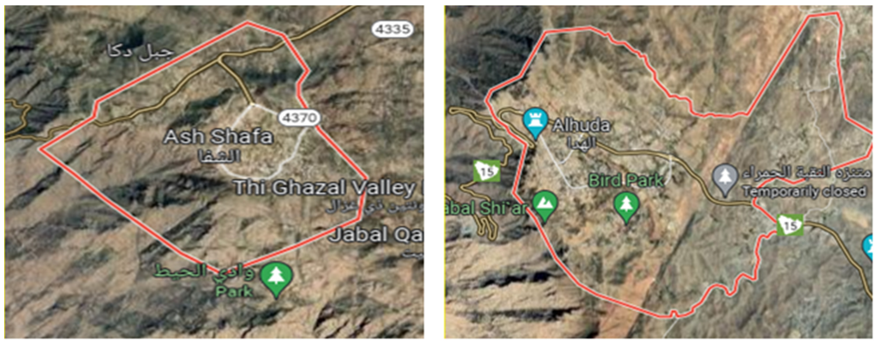
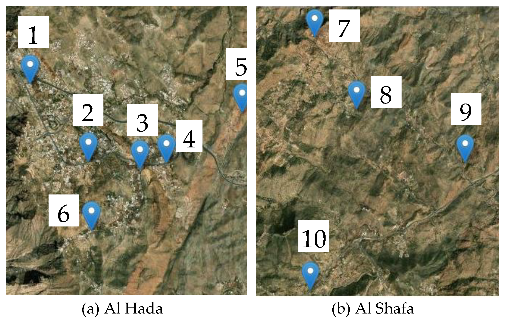
3.1. Study Area
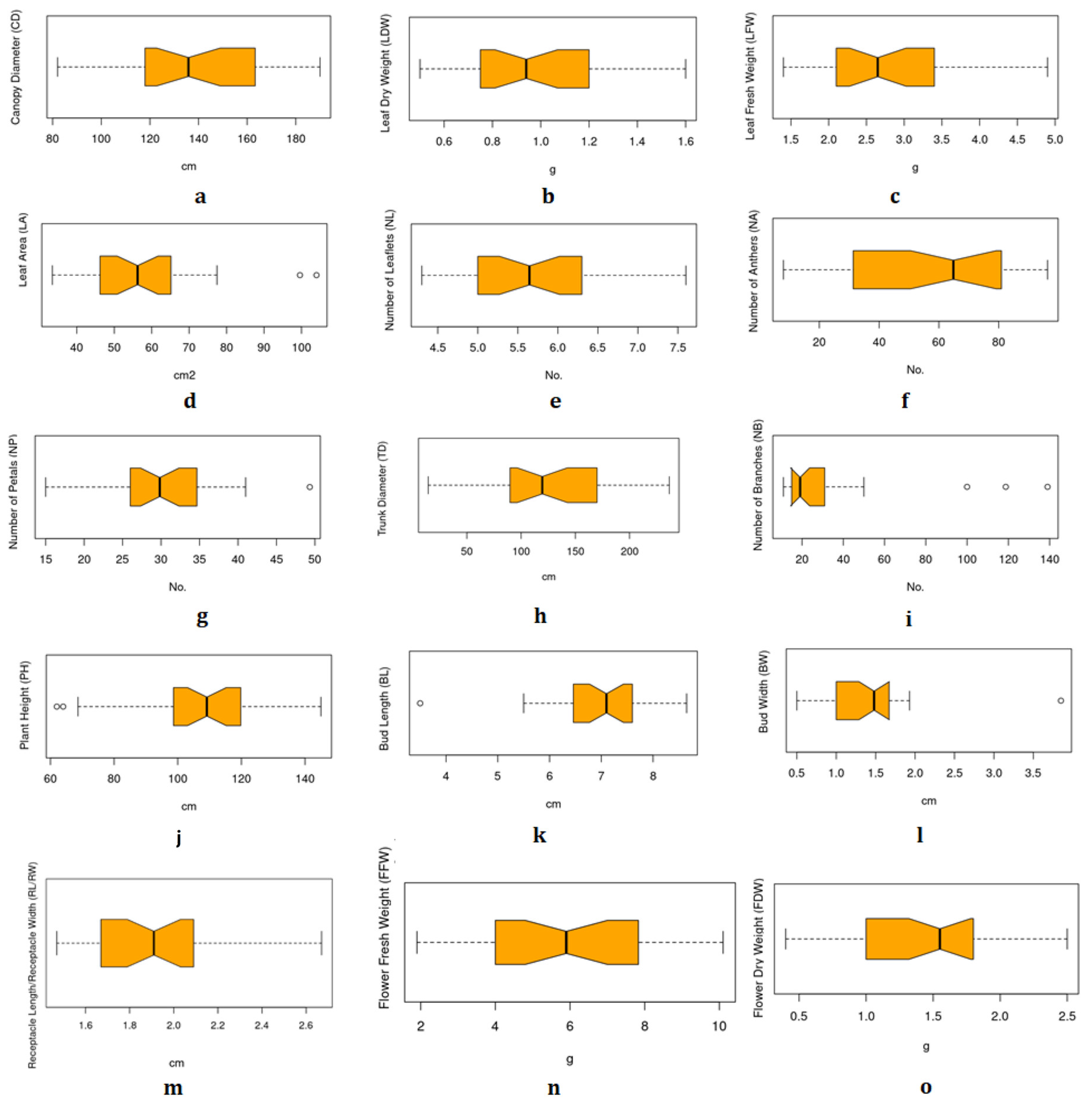
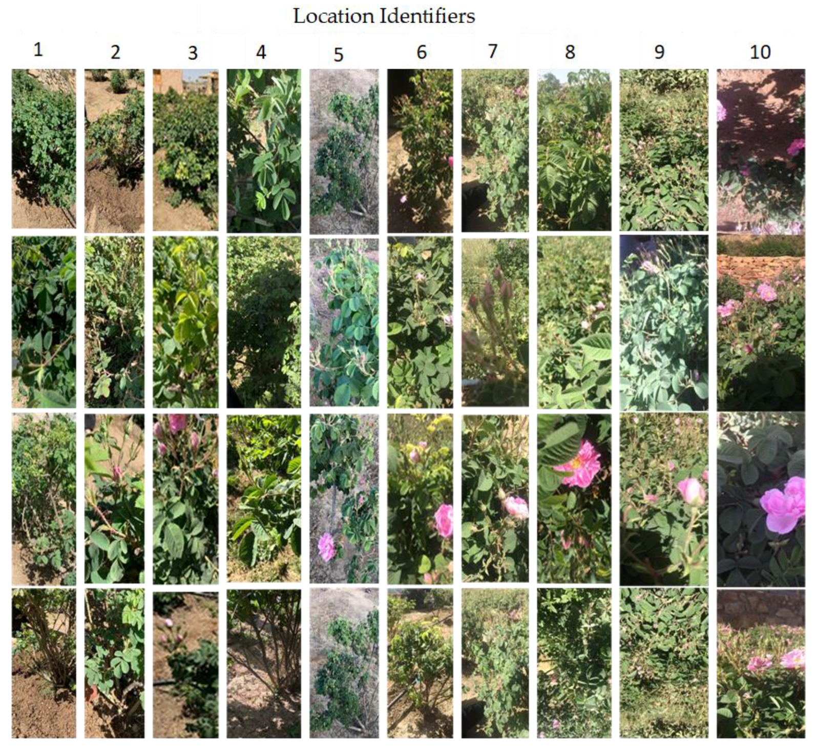
3.2. Phenotyping Datasets
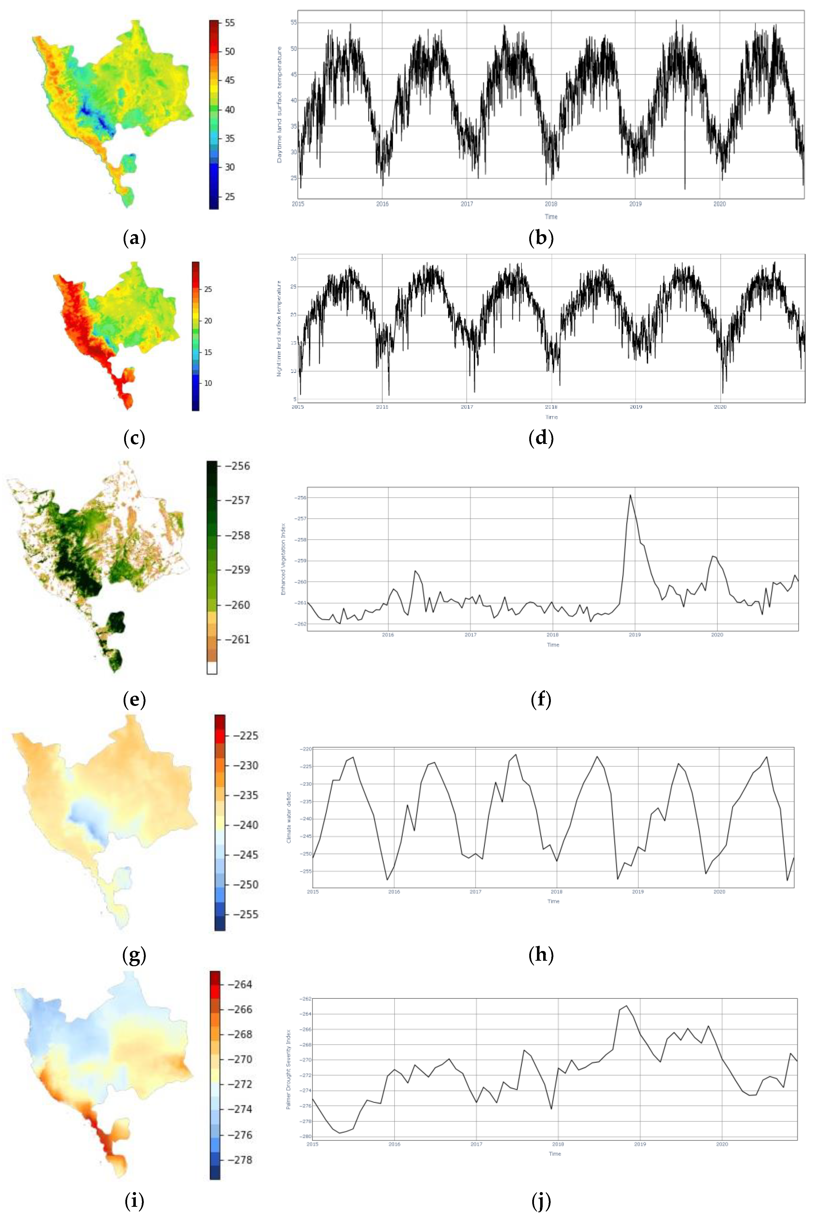
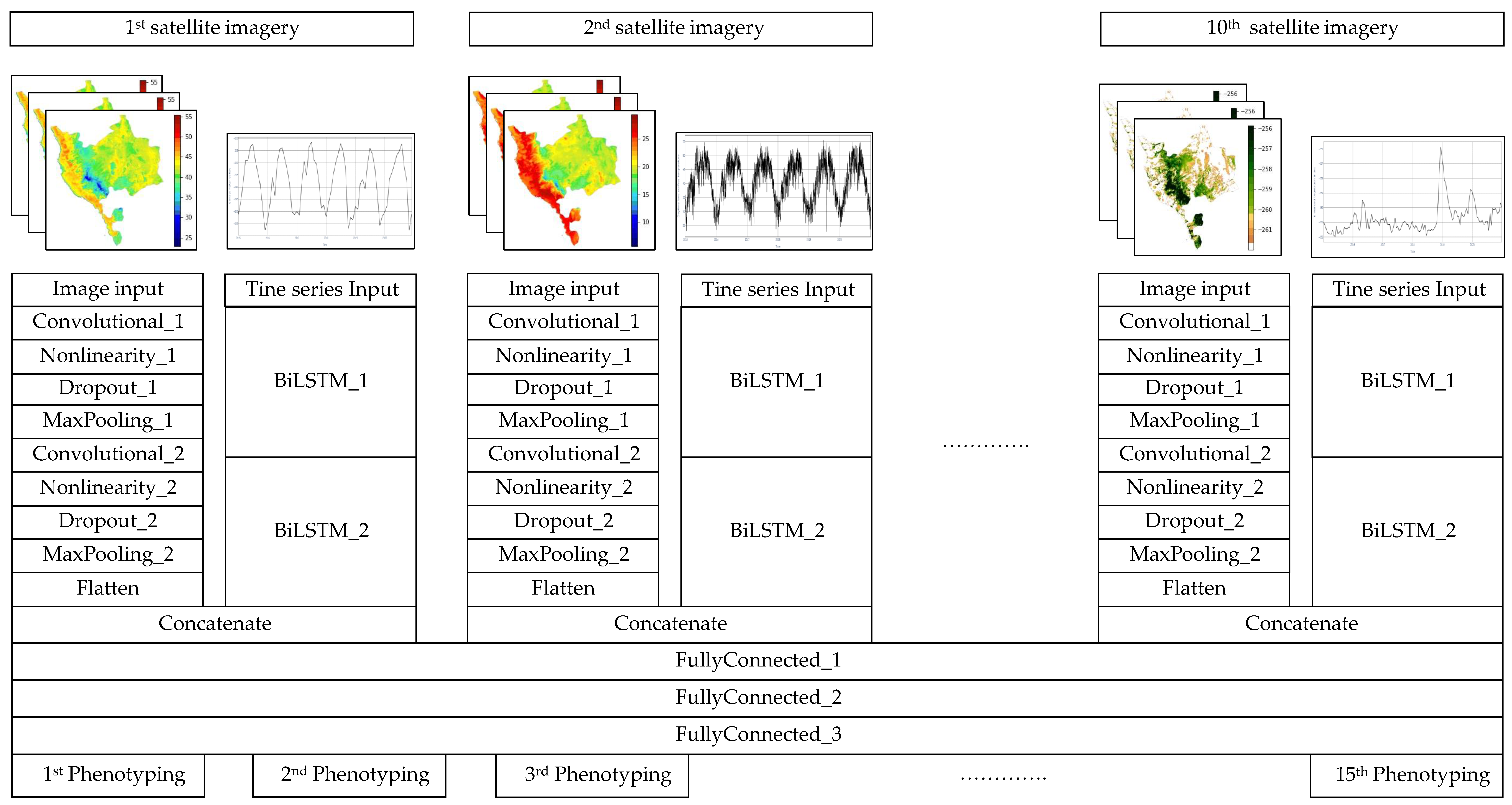
3.3. Satellite Imageries Datasets

| Dataset Name | Unit | Dataset Size | Spatial Resolution (m) | Temporal Resolution |
|---|---|---|---|---|
| Daytime Land surface Temperature (DLT) [67] | Celsius | 365 | 1000 | Daily |
| Nighttime land surface Temperature (NLT) [67] | Celsius | 365 | 1000 | Daily |
| Normalized Difference Vegetation Index (NDVI) [68] | None | 104 | 500 | Bimonthly |
| Enhanced Vegetation Index (EVI) [68] | None | 104 | 500 | Bimonthly |
| Actual Evapotranspiration (AE) [69] | mm | 12 | 4638.3 | Monthly |
| Climate Water Deficit (CWD) [69] | mm | 12 | 4638.3 | Monthly |
| Palmer Drought Severity Index (PDSI) [69] | mm | 12 | 4638.3 | Monthly |
| Runoff (Roff) [69]. | mm | 12 | 4638.3 | Monthly |
| Vapor Pressure Deficit (VPD) [69] | mm | 12 | 4638.3 | Monthly |
4. Methods
4.1. Convolution Neural Network
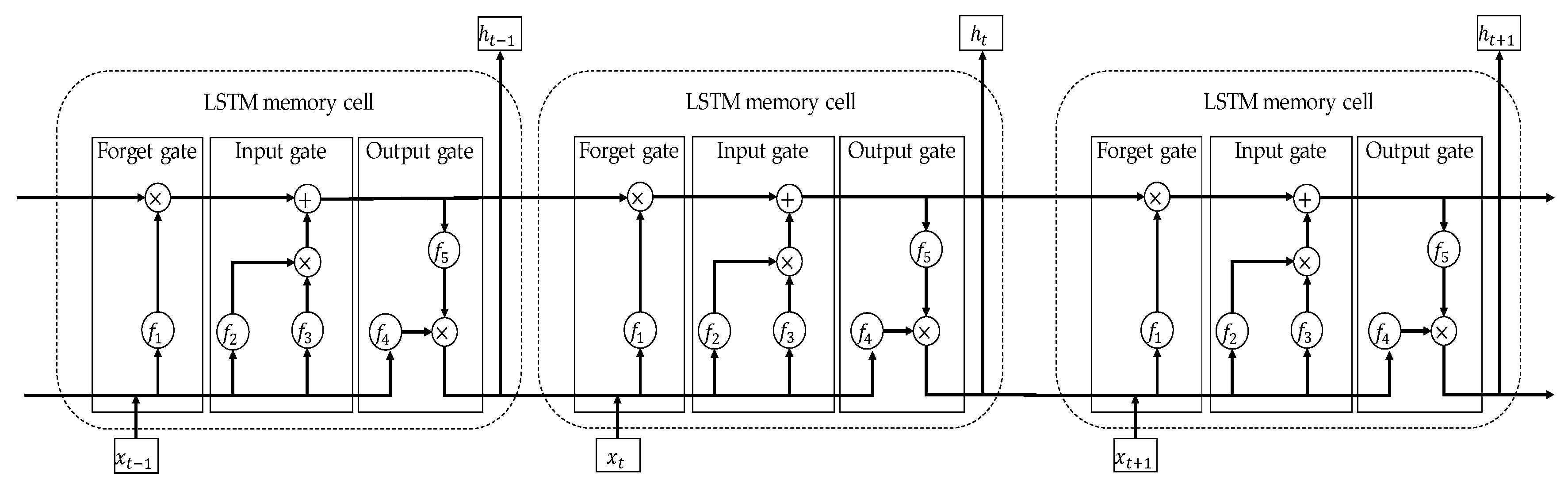
4.2. Long Short-Term Memory
4.3. The Proposed Model
5. Results and Discussion
5.1. Assessing the Complementary and Contextualization Learning Approaches
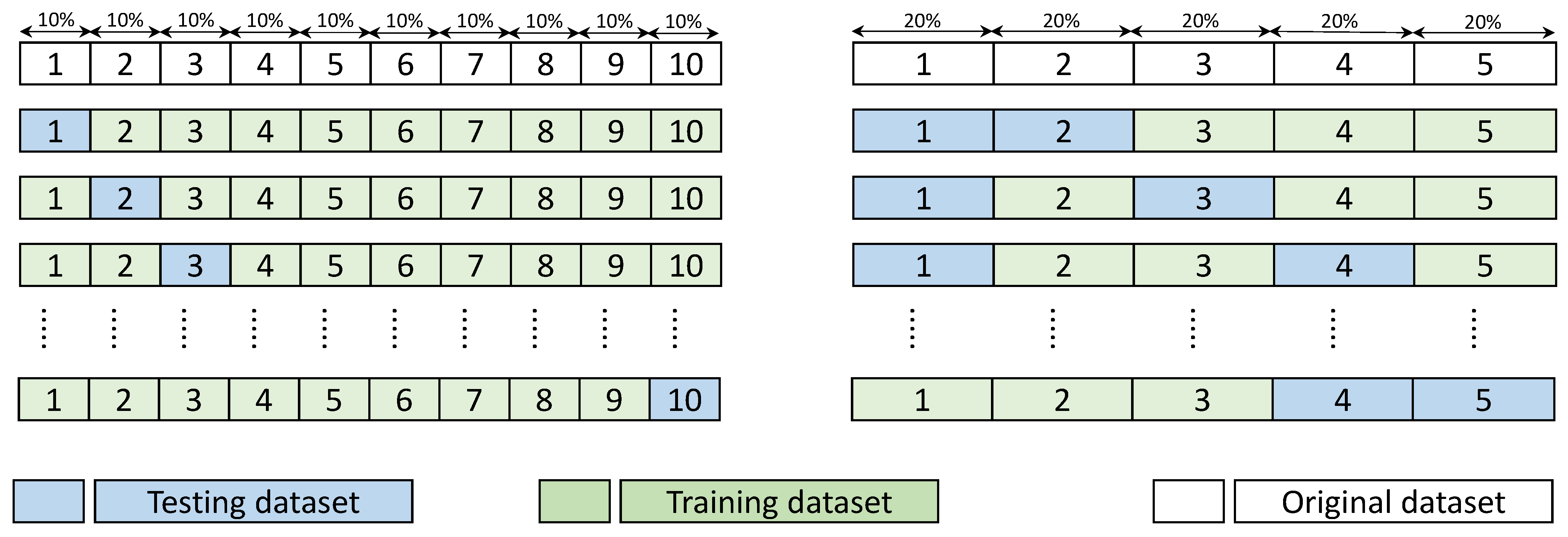
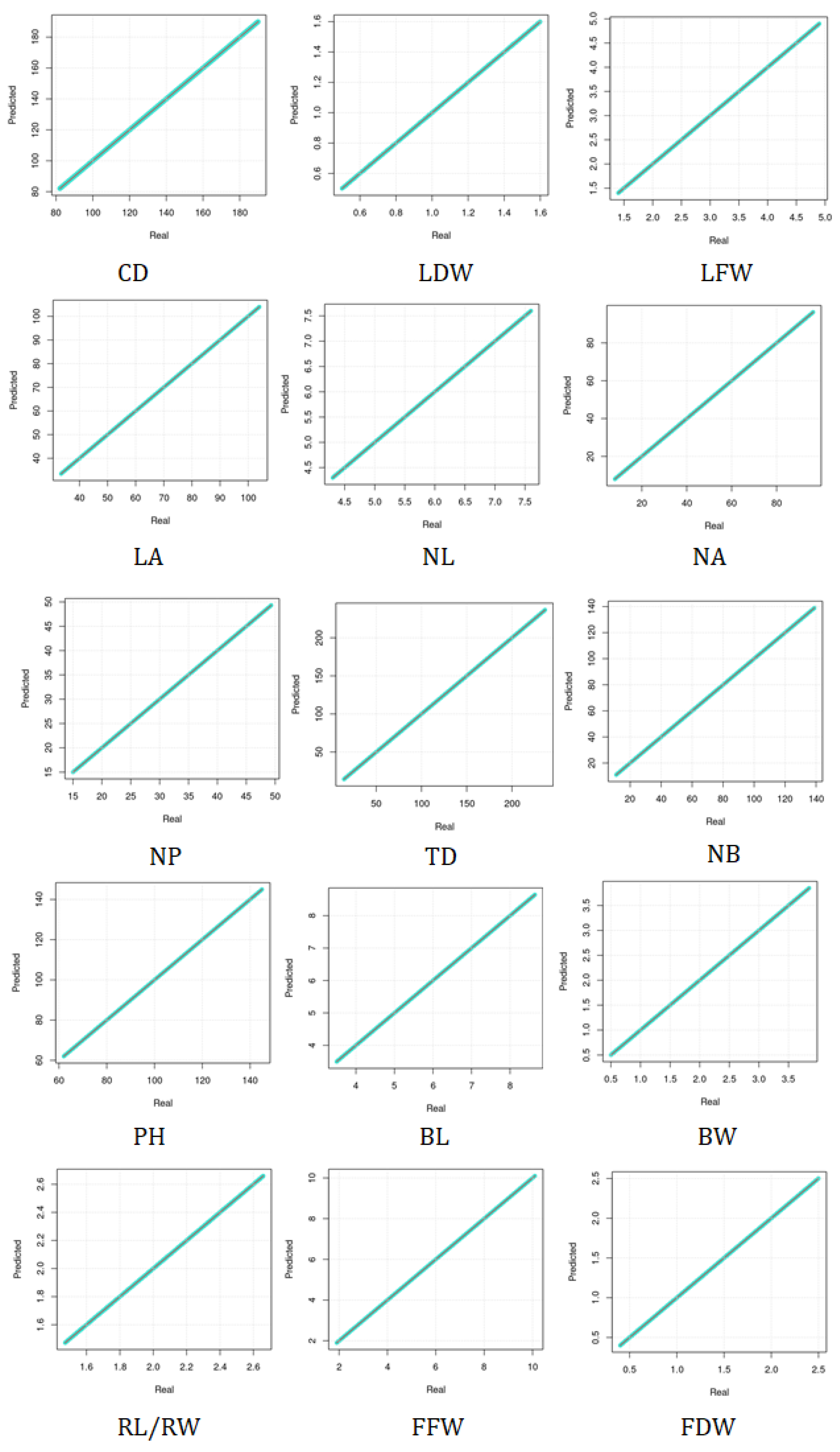
5.2. Assessing the Performance under Training and Testing Datasets
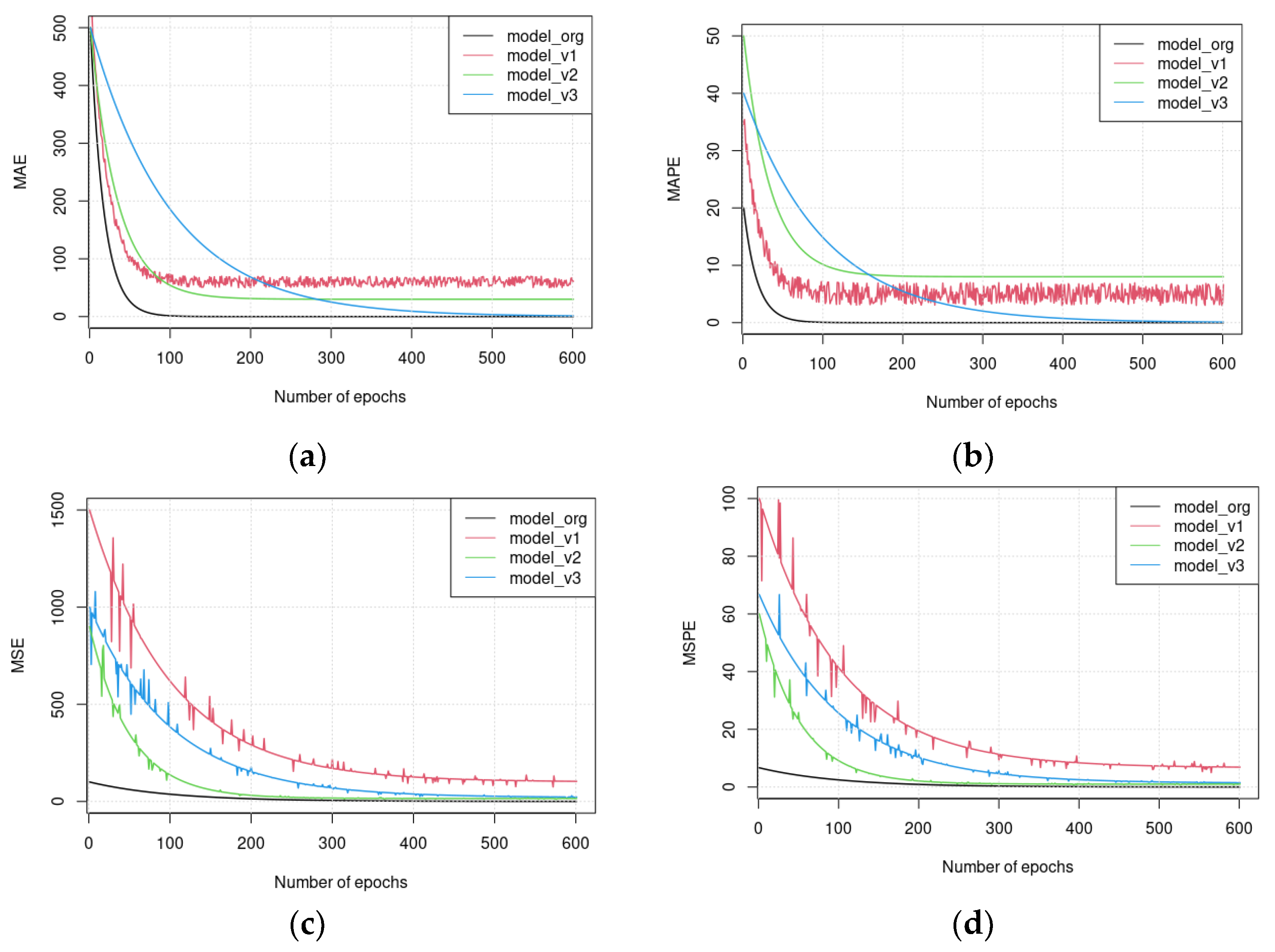
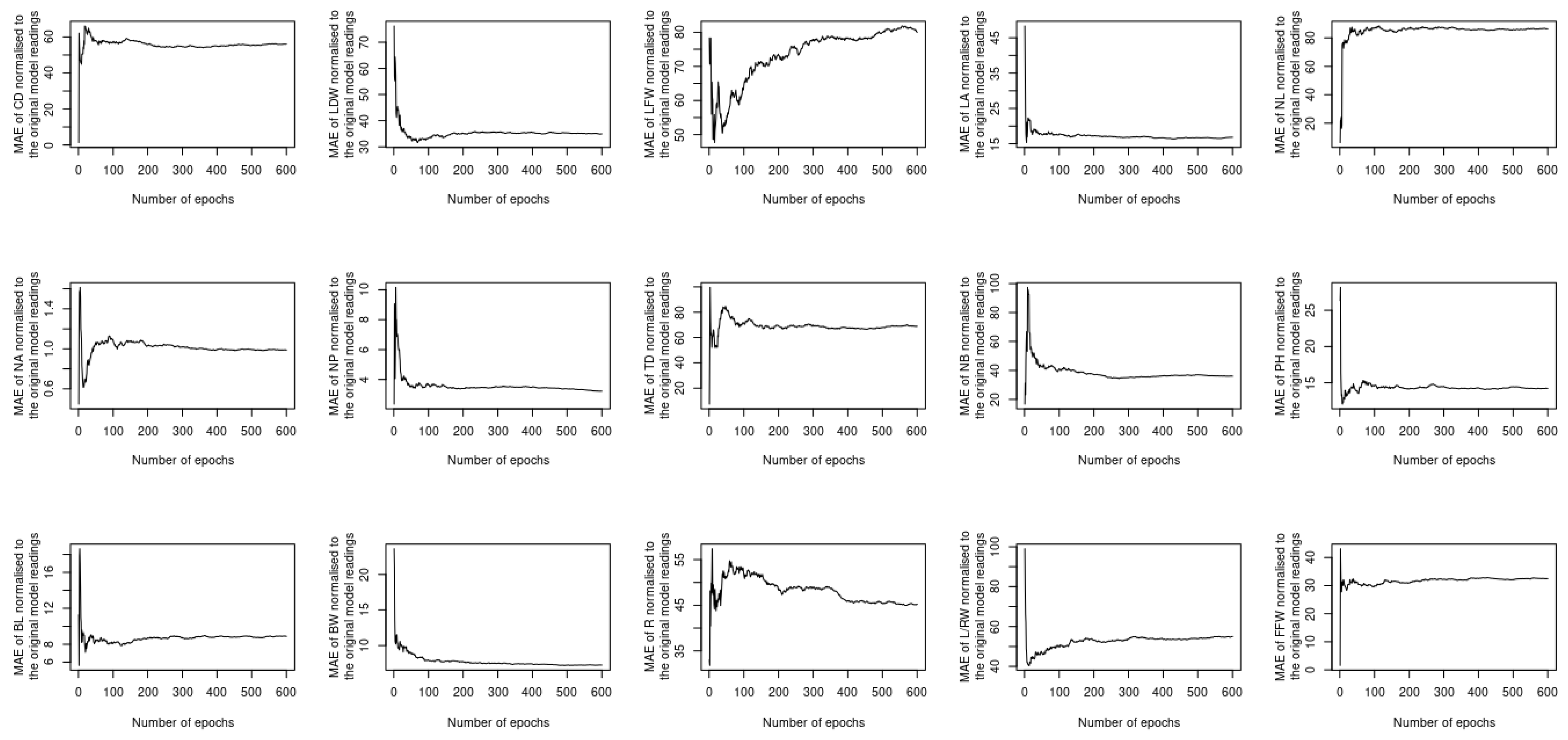
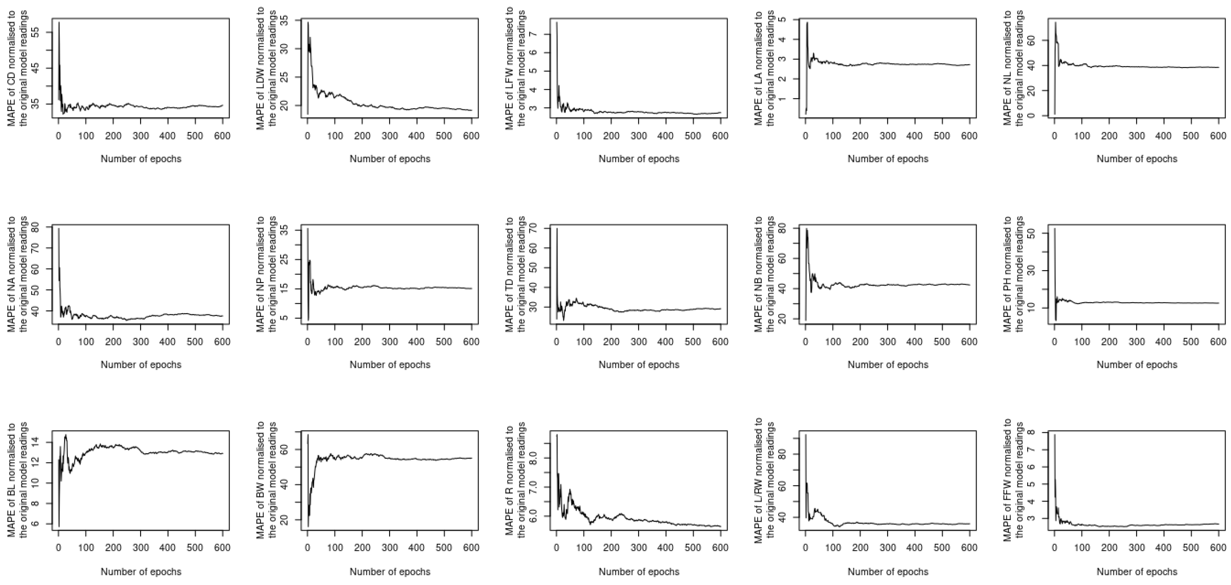
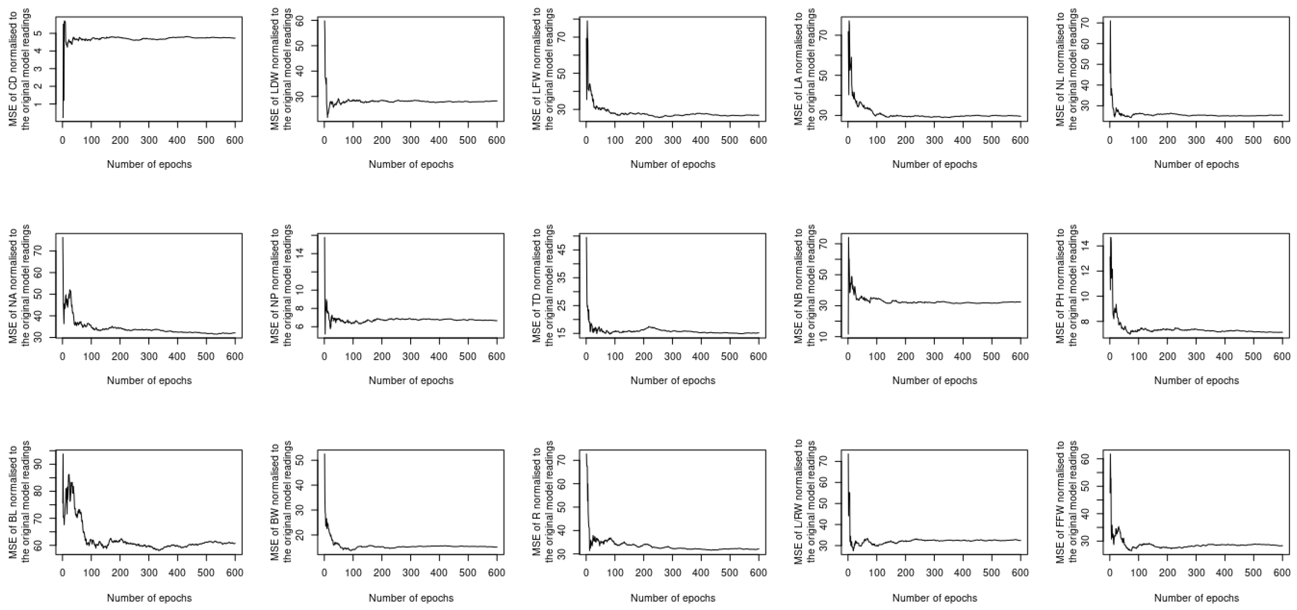
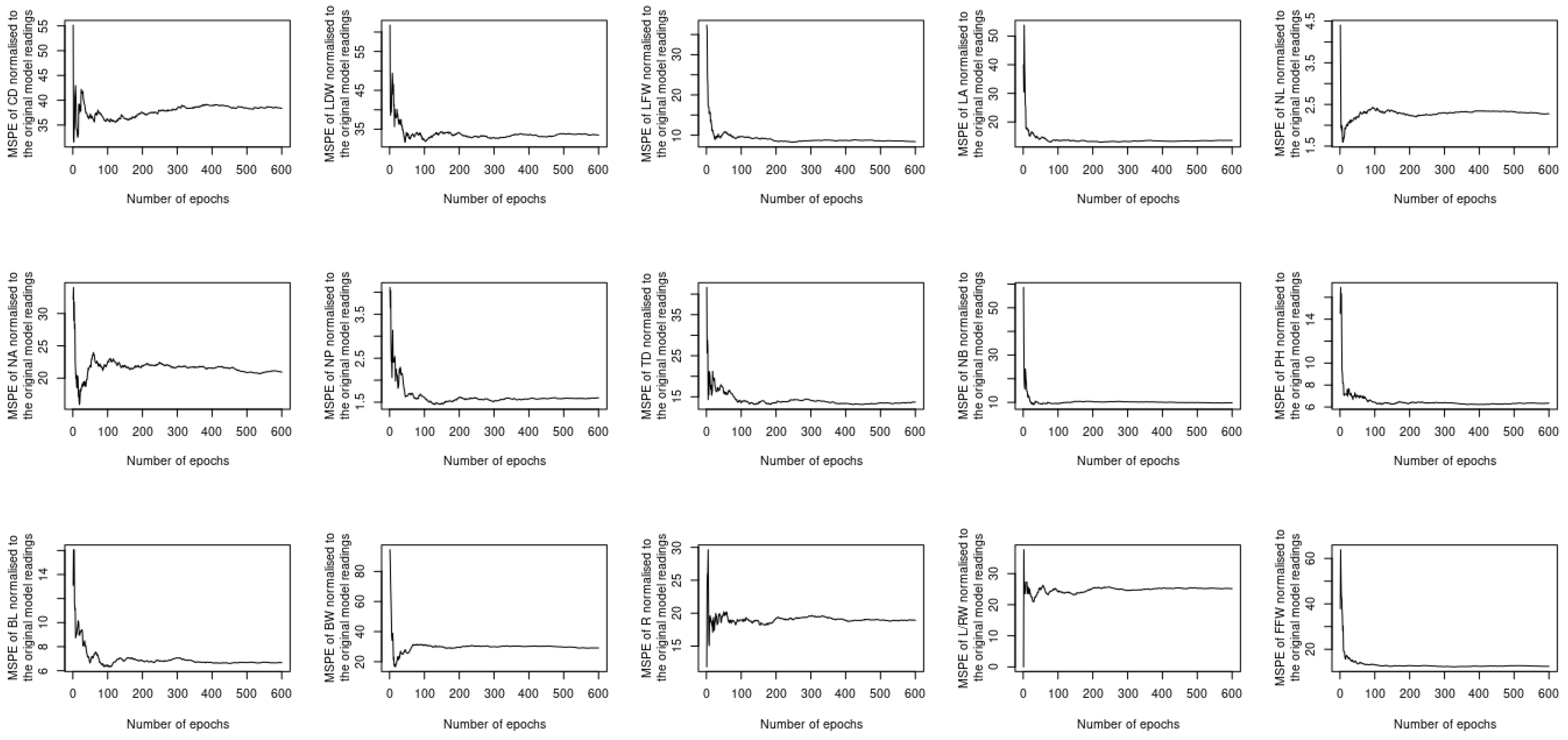
5.3. Assessment of Different Loss Functions
6. Conclusions and Future Work
Author Contributions
Funding
Data Availability Statement
Acknowledgments
Conflicts of Interest
References
- Rusanov, K.; Kovacheva, N.; Vosman, B.; Zhang, L.; Rajapakse, S.; Atanassov, A.; Atanassov, I. Microsatellite analysis of Rosa damascena Mill. accessions reveal genetic similarity between genotype s used for rose oil pro-duction and old Damask rose varieties. Theor. Appl. Genet. 2005, 111, 804–809. [Google Scholar] [CrossRef]
- Kashefi, B.; Matinizadeh, M.; Tabaei-Aghdaei, S.R. Superoxide dismutase and α-amylase changes of Damask rose (Rosa damascena Mill.) tissues seasonally. Afr. J. Agric. Res. 2012, 7, 5671–5679. [Google Scholar]
- Teo, C.J.; Chin, S.Y.; Wong, C.K.; Tan, C.C.; Goh, K.J. Planting Materials for High Sustainable Oil Palm Yields. In Proceedings of the Malaysian Oil Science and Technology (MOST); Malaysian Oil Scientists’ and Technologists’ Association: Petaling Jaya, Malaysia, 2017; Volume 26, pp. 58–119. [Google Scholar]
- Niazian, M.; Sadat-Noori, S.A.; Abdipour, M.; Tohidfar, M.; Mortazavian, S.M.M. Image Processing and Artificial Neural Network-Based Models to Measure and Predict Physical Properties of Embryogenic Callus and Number of Somatic Embryos in Ajowan (Trachyspermum ammi (L.) Sprague). Vitr. Cell. Dev. Biol. Plant 2018, 54, 54–68. [Google Scholar] [CrossRef]
- Ahmad Latif, N.; Mohd Nain, F.N.; Ahamed Hassain Malim, N.H.; Abdullah, R.; Abdul Rahim, M.F.; Mohamad, M.N.; Mohamad Fauzi, N.S. Predicting Heritability of Oil Palm Breeding Using Phenotypic Traits and Machine Learning. Sustainability 2021, 13, 12613. [Google Scholar] [CrossRef]
- Eli-Chukwu, N.; Ogwugwam, E.C. Applications of Artificial Intelligence in Agriculture: A Review. J. Eng. Technol. Appl. Sci. Res. 2019, 9, 4377–4383. [Google Scholar] [CrossRef]
- Yoosefzadeh-Najafabadi, M.; Earl, H.J.; Tulpan, D.; Sulik, J.; Eskandari, M. Application of Machine Learning Algorithms in Plant Breeding: Predicting Yield From Hyperspectral Reflectance in Soybean. Front. Plant Sci. 2021, 11, 624273. [Google Scholar] [CrossRef]
- Jung, M.; Song, J.S.; Hong, S.; Kim, S.; Go, S.; Lim, Y.P.; Park, J.; Park, S.G.; Kim, Y.-M. Deep Learning Algorithms Correctly Classify Brassica rapa Varieties Using Digital Images. Front. Plant Sci. 2021, 12, 738685. [Google Scholar] [CrossRef]
- Sandhu, K.S.; Lozada, D.N.; Zhang, Z.; Pumphrey, M.O.; Carter, A.H. Deep Learning for Predicting Complex Traits in Spring Wheat Breeding Program. Front. Plant Sci. 2021, 11, 613325. [Google Scholar] [CrossRef]
- Rutkoski, J.; Poland, J.; Mondal, S.; Autrique, E.; Pérez, L.G.; Crossa, J.; Reynolds, M.P.; Singh, R. Canopy Temperature and Vegetation Indices from High-Throughput Phenotyping Improve Accuracy of Pedigree and Genomic Selection for Grain Yield in Wheat. G3 Genes Genomes Genet. 2016, 6, 2799–2808. [Google Scholar] [CrossRef] [Green Version]
- Araus, J.L.; Cairns, J.E. Field high-throughput phenotyping: The new crop breeding frontier. Trends Plant Sci. 2014, 19, 52–61. [Google Scholar] [CrossRef]
- Tardieu, F.; Cabrera-Bosquet, L.; Pridmore, T.; Bennett, M. Plant phenomics, from sensors to knowledge. Curr. Biol. 2017, 27, R770–R783. [Google Scholar] [CrossRef]
- Araus, J.L.; Kefauver, S.C.; Zaman-Allah, M.; Olsen, M.S.; Cairns, J.E. Translating high-throughput phenotyping into genetic gain. Trends Plant Sci. 2018, 23, 451–466. [Google Scholar] [CrossRef] [PubMed] [Green Version]
- Lopez-Cruz, M.; Olson, E.; Rovere, G.; Crossa, J.; Dreisigacker, S.; Mondal, S.; Singh, R.P.; Campos, G.D.L. Regularized selection indices for breeding value prediction using hyper-spectral image data. Sci. Rep. 2020, 10, 8195. [Google Scholar] [CrossRef] [PubMed]
- Hesami, M.; Jones, A.M.P. Application of artificial intelligence models and optimization algorithms in plant cell and tissue culture. Appl. Microbiol. Biotechnol. 2020, 104, 9449–9485. [Google Scholar] [CrossRef] [PubMed]
- Pal, S.; Mitra, S. Multilayer perceptron, fuzzy sets, and classification. IEEE Trans. Neural Netw. 1992, 3, 683–697. [Google Scholar] [CrossRef] [PubMed]
- Geetha, M. Forecasting the crop yield production in trichy district using fuzzy C-Means algorithm and multilayer pceptron (MLP). Int. J. Knowl. Syst. Sci. (IJKSS) 2020, 11, 83–98. [Google Scholar] [CrossRef]
- Min, S.; Lee, B.; Yoon, S. Deep learning in bioinformatics. Brief. Bioinform. 2017, 18, 851–869. [Google Scholar] [CrossRef] [PubMed] [Green Version]
- Angermueller, C.; Pärnamaa, T.; Parts, L.; Stegle, O. Deep learning for computational biology. Mol. Syst. Biol. 2016, 12, 878. [Google Scholar] [CrossRef]
- Wang, H.; Cimen, E.; Singh, N.; Buckler, E. Deep learning for plant genomics and crop improvement. Curr. Opin. Plant Biol. 2020, 54, 34–41. [Google Scholar] [CrossRef]
- Rangarajan, A.K.; Purushothaman, R.; Ramesh, A. Tomato crop disease classification using pre-trained deep learning algorithm. Procedia Comput. Sci. 2018, 133, 1040–1047. [Google Scholar] [CrossRef]
- Abdulridha, J.; Ampatzidis, Y.; Roberts, P.; Kakarla, S.C. Detecting powdery mildew disease in squash at different stages using UAV-based hyperspectral imaging and artificial intelligence. Biosyst. Eng. 2020, 197, 135–148. [Google Scholar] [CrossRef]
- Pahikkala, T.; Kari, K.; Mattila, H.; Lepistö, A.; Teuhola, J.; Nevalainen, O.; Tyystjärvi, E. Classification of plant species from images of overlapping leaves. Comput. Electron. Agric. 2015, 118, 186–192. [Google Scholar] [CrossRef]
- Mouine, S.; Yahiaoui, I.; Verroust-Blondet, A. A shape-based approach for leaf classification using multiscale triangular representation. In Proceedings of the ICMR’13—3rd ACM International Conference on Multimedia Retrieval, Dallas, TX, USA, 16–20 April 2013. [Google Scholar]
- Schikora, M.; Schikora, A.; Kogel, K.; Koch, W.; Cremers, D. Probabilistic classification of disease symptoms caused by salmonella on Arabidopsis plants. GI Jahrestag 2010, 10, 874–879. [Google Scholar]
- Fahlgren, N.; Feldman, M.; Gehan, M.A.; Wilson, M.S.; Shyu, C.; Bryant, D.W.; Hill, S.T.; McEntee, C.J.; Warnasooriya, S.N.; Kumar, I.; et al. A versatile phenotyping system and analytics platform reveals diverse temporal responses to water availability in setaria. Mol. Plant. 2015, 8, 1520–1535. [Google Scholar] [CrossRef] [Green Version]
- Haug, S.; Michaels, A.; Biber, P.; Ostermann, J. Plant classification system for crop/weed discrimination without segmentation. In Proceedings of the IEEE Winter Conference on Applications of Computer Vision, Steamboat Springs, CO, USA, 24–26 March 2014. [Google Scholar]
- Singh, A.; Ganapathysubramanian, B.; Singh, A.K.; Sarkar, S. Machine learning for high-throughput stress phenotyping in plants. Trends Plant Sci. 2016, 21, 110–124. [Google Scholar] [CrossRef] [Green Version]
- Tsaftaris, S.A.; Minervini, M.; Scharr, H. Machine learning for plant phenotyping needs image processing. Trends Plant Sci. 2016, 21, 989–991. [Google Scholar] [CrossRef] [Green Version]
- Suh, H.K.; Ijsselmuiden, J.; Hofstee, J.W.; van Henten, E.J. Transfer learning for the classification of sugar beet and volunteer potato under field conditions. Biosyst. Eng. 2018, 174, 50–65. [Google Scholar] [CrossRef]
- Argüeso, D.; Picon, A.; Irusta, U.; Medela, A.; San-Emeterio, M.G.; Bereciartua, A.; Alvarez-Gila, A. Few-shot learning approach for plant disease classification using images taken in the field. Comput. Electron. Agric. 2020, 175, 105542. [Google Scholar] [CrossRef]
- Abbas, A.; Jain, S.; Gour, M.; Vankudothu, S. Tomato plant disease detection using transfer learning with C-GAN synthetic images. Comput. Electron. Agric. 2021, 187, 106279. [Google Scholar] [CrossRef]
- Khaki, S.; Pham, H.; Han, Y.; Kuhl, A.; Kent, W.; Wang, L. Deepcorn: A semi-supervised deep learning method for high-throughput image-based corn kernel counting and yield estimation. Knowl. Based Syst. 2021, 218, 106874. [Google Scholar] [CrossRef]
- Goodfellow, I.; Bengio, Y.; Courville, A. Deep Learning; MIT Press: London, UK, 2016; Available online: https://books.google.com/books/about/Deep_Learning.html?hl=&id=Np9SDQAAQBAJ (accessed on 15 February 2022).
- Kamilaris, A.; Prenafeta-Boldú, F.X. Deep learning in agriculture: A survey. Comput. Electron. Agric. 2018, 147, 70–90. [Google Scholar] [CrossRef] [Green Version]
- González-Recio, O.; Forni, S. Genome-wide prediction of discrete traits using Bayesian regressions and machine learning. Genet. Sel. Evol. 2011, 43, 7. [Google Scholar] [CrossRef] [PubMed] [Green Version]
- González-Recio, O.; Jiménez-Montero, J.A.; Alenda, R. The gradient boosting algorithm and random boosting for genome assisted evaluation in large data sets. J. Dairy Sci. 2013, 96, 614–624. [Google Scholar] [CrossRef] [PubMed] [Green Version]
- Pound, M.P.; Atkinson, J.A.; Pridmore, T.P.; Wells, D.M.; French, A.P. Deep Learning for Multi-task Plant Phenotyping. In Proceedings of the 2017 IEEE International Conference on Computer Vision Workshops (ICCVW), Venice, Italy, 22–29 October 2017. [Google Scholar] [CrossRef] [Green Version]
- Shi, W.; Van de Zedde, R.; Jiang, H.; Kootstra, G. Plant-part segmentation using deep learning and multi-view vision. Biosyst. Eng. 2019, 187, 81–95. [Google Scholar] [CrossRef]
- Taghavi Namin, S.; Esmaeilzadeh, M.; Najafi, M.; Brown, T.B.; Borevitz, J.O. Deep phenotyping: Deep learning for temporal phenotype/genotype classification. Plant Methods 2018, 14, 66. [Google Scholar] [CrossRef] [Green Version]
- Fang, B.; Lakshmi, V.; Bindlish, R.; Jackson, T.J.; Cosh, M.; Basara, J. Passive Microwave Soil Moisture Downscaling Using Vegetation Index and Skin Surface Temperature. Vadose Zone J. 2013, 12. [Google Scholar] [CrossRef]
- Mahdianpari, M.; Salehi, B.; Rezaee, M.; Mohammadimanesh, F.; Zhang, Y. Very Deep Convolutional Neural Networks for Complex Land Cover Mapping Using Multispectral Remote Sensing Imagery. Remote Sens. 2018, 10, 1119. [Google Scholar] [CrossRef] [Green Version]
- Sakurai, S.; Uchiyama, H.; Shimada, A.; Taniguchi, R. Plant Growth Prediction using Convolutional LSTM. In Proceedings of the 14th International Joint Conference on Computer Vision, Imaging and Computer Graphics Theory and Applications (VISIGRAPP 2019), Prague, Czech Republic, 25–27 February 2019; pp. 105–113. [Google Scholar] [CrossRef]
- Yasrab, R.; Zhang, J.; Smyth, P.; Pound, M.P. Predicting Plant Growth from Time-Series Data Using Deep Learning. Remote Sens. 2021, 13, 331. [Google Scholar] [CrossRef]
- Mishra, A.M.; Harnal, S.; Mohiuddin, K.; Gautam, V.; Nasr, O.A.; Goyal, N.; Alwetaishi, M.; Singh, A. A Deep Learning-Based Novel Approach for Weed Growth Estimation. Intell. Autom. Soft Comput. 2022, 31, 1157–1173. [Google Scholar] [CrossRef]
- Xi, Y.; Ren, C.; Wang, Z.; Wei, S.; Bai, J.; Zhang, B.; Xiang, H.; Chen, L. Mapping Tree Species Composition Using OHS-1 Hyperspectral Data and Deep Learning Algorithms in Changbai Mountains, Northeast China. Forests 2019, 10, 818. [Google Scholar] [CrossRef] [Green Version]
- Zhang, M.; Lin, H.; Wang, G.; Sun, H.; Fu, J. Mapping Paddy Rice Using a Convolutional Neural Network (CNN) with Landsat 8 Datasets in the Dongting Lake Area, China. Remote Sens. 2018, 10, 1840. [Google Scholar] [CrossRef] [Green Version]
- Du, L.; McCarty, G.W.; Zhang, X.; Lang, M.W.; Vanderhoof, M.K.; Li, X.; Huang, C.; Lee, S.; Zou, Z. Mapping Forested Wetland Inundation in the Delmarva Peninsula, USA Using Deep Convolutional Neural Networks. Remote Sens. 2020, 12, 644. [Google Scholar] [CrossRef] [Green Version]
- Ma, J.; Li, Y.; Chen, Y.; Du, K.; Zheng, F.; Zhang, L.; Sun, Z. Estimating above ground biomass of winter wheat at early growth stages using digital images and deep convolutional neural network. Eur. J. Agron. 2019, 103, 117–129. [Google Scholar] [CrossRef]
- Dong, L.; Du, H.; Han, N.; Li, X.; Zhu, D.; Mao, F.; Zhang, M.; Zheng, J.; Liu, H.; Huang, Z.; et al. Application of Convolutional Neural Network on Lei Bamboo Above-Ground-Biomass (AGB) Estimation Using Worldview-2. Remote Sens. 2020, 12, 958. [Google Scholar] [CrossRef] [Green Version]
- Li, W.; Fu, H.; Yu, L.; Cracknell, A. Deep Learning Based Oil Palm Tree Detection and Counting for High-Resolution Remote Sensing Images. Remote Sens. 2017, 9, 22. [Google Scholar] [CrossRef] [Green Version]
- Malambo, L.; Popescu, S.; Ku, N.-W.; Rooney, W.; Zhou, T.; Moore, S. A Deep Learning Semantic Segmentation-Based Approach for Field-Level Sorghum Panicle Counting. Remote Sens. 2019, 11, 2939. [Google Scholar] [CrossRef] [Green Version]
- Alqurashi, A.F.; Kumar, L. Land Use and Land Cover Change Detection in the Saudi Arabian Desert Cities of Makka and Al-Taif Using Satellite Data. Adv. Remote Sens. 2014, 3, 106–119. [Google Scholar] [CrossRef]
- Abdullh, M.A.; AL-Yasee, H.; AL-Sudani, Y.; Khandaker, M.M. Developing weeds of Agricultural Crops at different levels of Heights, in Taif Area Of Saudia Arabia. Bulg. J. Agric. Sci. 2017, 23, 762–769. Available online: https://www.researchgate.net/publication/320864744 (accessed on 15 February 2022).
- Climate Atlas of Saudi Arabia; Ministry of Agriculture and Water: Riyad, United Arab Emirates, 1990.
- Ady, J. The Taif Escarpment, Saudi Arabia: A Study For Nature Conservation And Recreational Development. Mt. Res. Dev. 1995, 15, 101–120. [Google Scholar] [CrossRef]
- Majrashi, A.; Khandaker, M.M. Survey of Portulacaceae family flora in Taif, Saudi Arabia. Braz. J. Biol. 2021, 84, e249230. [Google Scholar] [CrossRef]
- Beeson, R.C. Ribulose 1, 5-bisphosphate carboxylase/oxygenase activities in leaves of greenhouse roses. J. Exp. Bot. 1990, 41, 59–65. [Google Scholar] [CrossRef]
- Kool, M.T.N.; Westerman, A.D.; Rou-Haest, C.H.M. Importance and use of carbohydrate reserves in above-ground stem parts of rose cv. Motrea. J. Hort Sci. 1996, 71, 893–900. [Google Scholar] [CrossRef]
- Bredmose, N.B. Growth, flowering, and postharvest performance of single-stemmed rose (Rosa hibrida L.) plants in response to light quantum integral and plant population density. J. Am. Soc. Hortic. Sci. 1998, 123, 569–576. [Google Scholar] [CrossRef] [Green Version]
- Gonzalez-Real, M.M.; Baille, A. Change in leaf photosynthetic parameters with leaf position and nitrogen content within a rose plant canopy (Rosa hibrida). Plant Cell Environ. 2000, 23, 351–363. [Google Scholar] [CrossRef]
- Kim, S.H.; Lieth, J.H. A coupled model of photosynthesis, stomatal conductance, and transpiration for a rose leaf (Rosa hybrida L.). Ann. Bot. 2003, 9, 771–781. [Google Scholar] [CrossRef] [PubMed] [Green Version]
- Weiss, E.A. Essential Oil Crops; CAB International: Wallingford, UK, 1997. [Google Scholar]
- Pal, P.K.; Singh, R. Understanding crop-ecology and agronomy of Rosa damascena Mill. for higher productivity. Aust. J. Crop Sci. 2013, 7, 196–205. [Google Scholar]
- Rusanov, K.E.; Kovacheva, N.M.; Atanassov, I.I. Comparative GC/MS analysis of Rose flower and distilled oil volatiles of the oil-bearing Rose Rosa Damascena. Biotechnol. Biotechnol. Eq. 2011, 25, 2210–2216. [Google Scholar] [CrossRef] [Green Version]
- Osorio-Guarín, J.A.S.; Garzón-Martínez, G.A.; Delgadillo-Duran, P.; Bastidas, S.; Moreno, L.P.; Enciso-Rodríguez, F.E.; Cornejo, O.E.; Barrero, L.S. Genome-wide association study (GWAS) for morphological and yield-related traits in an oil palm hybrid (Elaeis oleifera × Elaeis guineensis) population. BMC Plant Biol. 2019, 19, 533. [Google Scholar] [CrossRef] [Green Version]
- MOD11A1.006 Terra Land Surface Temperature and Emissivity Daily Global 1 km|Earth Engine Data Catalog|Google Developers. Available online: https://developers.google.com/earth-engine/datasets/catalog/MODIS_006_MOD11A1 (accessed on 15 February 2022).
- MYD13A2.006 Aqua Vegetation Indices 16-Day Global 1 km|Earth Engine Data Catalog|Google Developers. Available online: https://developers.google.com/earth-engine/datasets/catalog/MODIS_006_MYD13A2 (accessed on 15 February 2022).
- TerraClimate: Monthly Climate and Climatic Water Balance for Global Terrestrial Surfaces, University of Idaho|Earth Engine Data Catalog|Google Developers. Available online: https://developers.google.com/earth-engine/datasets/catalog/IDAHO_EPSCOR_TERRACLIMATE (accessed on 15 February 2022).
- da Silva, I.N.; Spatti, D.H.; Flauzino, R.A.; Liboni, L.H.B.; dos Reis Alves, S.F. Artificial Neural Networks: A Practical Course—Google Books; Springer International Publishing: Basel, Switzerlands, 2017. [Google Scholar]
- Baz, A.; Baz, M. PCN2: Parallel CNN to Diagnose COVID-19 from Radiographs and Metadata. Intell. Autom. Soft Comput. 2022, 31, 1051–1069. [Google Scholar] [CrossRef]
| Layer Name | Dimensions | Input | Output | Number of Parameters | ||||||
|---|---|---|---|---|---|---|---|---|---|---|
| L | W | D | L | W | D | L | W | D | ||
| Image input | 255 | 255 | 3 | 255 | 255 | 3 | 255 | 255 | 3 | 0 |
| Convolutional_1 | 3 | 3 | 32 | 255 | 255 | 3 | 253 | 253 | 32 | 896 |
| Nonlinearltiy_1 | 3 | 3 | 32 | 253 | 253 | 32 | 253 | 253 | 32 | 0 |
| Dropout_1 | 0.4 | 253 | 253 | 32 | 253 | 253 | 32 | 0 | ||
| MaxPooiling_1 | 2 | 2 | 32 | 253 | 253 | 32 | 126 | 126 | 32 | 0 |
| Convolutional_2 | 3 | 3 | 32 | 126 | 126 | 32 | 124 | 124 | 32 | 9248 |
| Nonlinearltiy_2 | 124 | 124 | 32 | 124 | 124 | 32 | 124 | 124 | 32 | 0 |
| Dropout_2 | 0.4 | 124 | 124 | 32 | 124 | 124 | 32 | 0 | ||
| MaxPooiling_2 | 2 | 2 | 32 | 244 | 124 | 32 | 62 | 62 | 32 | 0 |
| Flatten | - | - | - | 62 | 62 | 32 | 1 | 1 | 123,008 | 0 |
| Timeseries input | Varies | 1 | 9 | Varies | 1 | 9 | Varies | 1 | 9 | 0 |
| BiLSTM_1 | Varies | 100 | 9 | Varies | 1 | 9 | Varies | 1 | 200 | 88,000 |
| BiLSTM_2 | Varies | 100 | 9 | Varies | 1 | 200 | Varies | 1 | 200 | 240,800 |
| Concatenate | - | - | - | Varies | 1 | 200 | 1 | 1 | 123,208 | 0 |
| 1 | 1 | 123,008 | ||||||||
| FullyConnected_1 | 1 | 100 | - | 1 | 1 | 1,230,080 | 1 | 1 | 100 | 123,208,100 |
| FullyConnected_2 | 1 | 100 | - | 1 | 1 | 100 | 1 | 1 | 100 | 10,100 |
| FullyConnected_3 | 1 | 10 | - | 1 | 1 | 100 | 1 | 1 | 15 | 1515 |
| Folds id | model_org | model_v1 | model_v2 | model_v3 | ||||||||||||
| Training | Testing | Training | Testing | Training | Testing | Training | Testing | |||||||||
| 9:1 training to testing datasets | ||||||||||||||||
| 1 | 0 | 0 | 0 | 0 | 8.44 × 10⁻⁶ | 4.50 × 10⁻⁷ | 1.41 × 10⁻⁶ | 6.95 × 10⁻⁶ | 7.85 × 10⁻⁶ | 7.66 × 10⁻⁶ | 9.90 × 10⁻⁷ | 7.70 × 10⁻⁷ | 1.00 × 10⁻⁶ | 4.50 × 10⁻⁷ | 5.10 × 10⁻⁷ | 1.90 × 10⁻⁷ |
| 2 | 0 | 0 | 0 | 0 | 6.72 × 10⁻⁶ | 1.69 × 10⁻⁶ | 2.80 × 10⁻⁷ | 9.11 × 10⁻⁶ | 8.27 × 10⁻⁶ | 5.44 × 10⁻⁶ | 7.02 × 10⁻⁶ | 7.57 × 10⁻⁶ | 1.10 × 10⁻⁷ | 1.35 × 10⁻⁶ | 9.90 × 10⁻⁶ | 5.60 × 10⁻⁶ |
| 3 | 0 | 0 | 0 | 0 | 8.29 × 10⁻⁶ | 5.48 × 10⁻⁶ | 1.25 × 10⁻⁶ | 3.01 × 10⁻⁶ | 2.77 × 10⁻⁶ | 5.60 × 10⁻⁶ | 7.98 × 10⁻⁶ | 4.50 × 10⁻⁷ | 2.84 × 10⁻⁶ | 7.32 × 10⁻⁶ | 7.48 × 10⁻⁶ | 1.91 × 10⁻⁶ |
| 4 | 0 | 0 | 0 | 0 | 6.5 × 10⁻⁶ | 7.95 × 10⁻⁶ | 1.14 × 10⁻⁶ | 8.29 × 10⁻⁶ | 8.90 × 10⁻⁶ | 7.90 × 10⁻⁶ | 5.78 × 10⁻⁶ | 3.18 × 10⁻⁶ | 6.27 × 10⁻⁶ | 3.62 × 10⁻⁶ | 3.56 × 10⁻⁶ | 9.97 × 10⁻⁶ |
| 5 | 0 | 0 | 0 | 0 | 1.53 × 10⁻⁶ | 4.20 × 10⁻⁷ | 4.4 × 10⁻⁶ | 8.89 × 10⁻⁶ | 6.24 × 10⁻⁶ | 2.22 × 10⁻⁶ | 7.64 × 10⁻⁶ | 4.80 × 10⁻⁶ | 6.18 × 10⁻⁶ | 7.86 × 10⁻⁶ | 1.17 × 10⁻⁶ | 1.92 × 10⁻⁶ |
| 6 | 0 | 0 | 0 | 0 | 2.76 × 10⁻⁶ | 4.55 × 10⁻⁶ | 9.20 × 10⁻⁶ | 5.69 × 10⁻⁶ | 8.01 × 10⁻⁶ | 7.35 × 10⁻⁶ | 8.53 × 10⁻⁶ | 6.97 × 10⁻⁶ | 2.41 × 10⁻⁶ | 8.88 × 10⁻⁶ | 8.13 × 10⁻⁶ | 1.20 × 10⁻⁶ |
| 7 | 0 | 0 | 0 | 0 | 5.72 × 10⁻⁶ | 3.7 × 10⁻⁶ | 6.19 × 10⁻⁶ | 9.86 × 10⁻⁶ | 5.6 × 10⁻⁶ | 6.83 × 10⁻⁶ | 5.63 × 10⁻⁶ | 9.43 × 10⁻⁶ | 3.33 × 10⁻⁶ | 4.91 × 10⁻⁶ | 9.17 × 10⁻⁶ | 8.10 × 10⁻⁶ |
| 8 | 0 | 0 | 0 | 0 | 5.17 × 10⁻⁶ | 8.55 × 10⁻⁶ | 2.88 × 10⁻⁶ | 2.48 × 10⁻⁶ | 1.70 × 10⁻⁶ | 8.08 × 10⁻⁶ | 5.73 × 10⁻⁶ | 7.87 × 10⁻⁶ | 3.95 × 10⁻⁶ | 5.17 × 10⁻⁶ | 3.52 × 10⁻⁶ | 6.73 × 10⁻⁶ |
| 9 | 0 | 0 | 0 | 0 | 4.15 × 10⁻⁶ | 4.88 × 10⁻⁶ | 2.71 × 10⁻⁶ | 2.82 × 10⁻⁶ | 3.18 × 10⁻⁶ | 6.5 × 10⁻⁶ | 5.89 × 10⁻⁶ | 6.83 × 10⁻⁶ | 3.23 × 10⁻⁶ | 5.23 × 10⁻⁶ | 5.39 × 10⁻⁶ | 1.76 × 10⁻⁶ |
| 10 | 0 | 0 | 0 | 0 | 9.84 × 10⁻⁶ | 9.52 × 10⁻⁶ | 3.68 × 10⁻⁶ | 9.25 × 10⁻⁶ | 3.46 × 10⁻⁶ | 9.52 × 10⁻⁶ | 9.00 × 10⁻⁷ | 7.81 × 10⁻⁶ | 7.85 × 10⁻⁶ | 9.5 × 10⁻⁶ | 9.13 × 10⁻⁶ | 4.92 × 10⁻⁶ |
| 5:2 training to testing datasets | ||||||||||||||||
| 1 | 0 | 0 | 0 | 0 | 2.01 × 10⁻⁴ | 6.76 × 10⁻⁴ | 3.67 × 10⁻⁴ | 3.19 × 10⁻⁴ | 4.80 × 10⁻⁴ | 8.72 × 10⁻⁴ | 3.51 × 10⁻⁴ | 9.37 × 10⁻⁴ | 7.64 × 10⁻⁴ | 5.90 × 10⁻⁴ | 9.96 × 10⁻⁴ | 1.13 × 10⁻⁴ |
| 2 | 0 | 0 | 0 | 0 | 8.95 × 10⁻⁴ | 9.61 × 10⁻⁴ | 4.40 × 10⁻⁵ | 5.70 × 10⁻⁵ | 8.83 × 10⁻⁴ | 4.02 × 10⁻⁴ | 4.7 × 10⁻⁴ | 8.14 × 10⁻⁴ | 8.30 × 10⁻⁴ | 9.21 × 10⁻⁴ | 5.24 × 10⁻⁴ | 7.08× 10⁻⁴ |
| 3 | 0 | 0 | 0 | 0 | 8.44 × 10⁻⁴ | 4.58 × 10⁻⁴ | 5.17 × 10⁻⁴ | 3.29 × 10⁻⁴ | 8.60 × 10⁻⁴ | 1.72 × 10⁻⁴ | 3.28 × 10⁻⁴ | 9.24 × 10⁻⁴ | 2.23 × 10⁻⁴ | 4.93 × 10⁻⁴ | 9.13 × 10⁻⁴ | 1.60 × 10⁻⁴ |
| 4 | 0 | 0 | 0 | 0 | 8.72 × 10⁻⁴ | 5.38 × 10⁻⁴ | 3.69 × 10⁻⁴ | 8.22 × 10⁻⁴ | 1.89 × 10⁻⁴ | 7.58 × 10⁻⁴ | 5.60 × 10⁻⁵ | 9.27 × 10⁻⁴ | 2.48 × 10⁻⁴ | 8.02 × 10⁻⁴ | 9.29 × 10⁻⁴ | 8.37 × 10⁻⁴ |
| 5 | 0 | 0 | 0 | 0 | 3.08 × 10⁻⁴ | 8.76 × 10⁻⁴ | 5.79 × 10⁻⁴ | 3.24 × 10⁻⁴ | 2.31 × 10⁻⁴ | 2.80 × 10⁻⁴ | 5.73 × 10⁻⁴ | 2.36 × 10⁻⁴ | 7.19 × 10⁻⁴ | 2.35 × 10⁻⁴ | 2.5 × 10⁻⁴ | 7.77 × 10⁻⁴ |
| 6 | 0 | 0 | 0 | 0 | 2.72 × 10⁻⁴ | 7.60 × 10⁻⁴ | 2.6 × 10⁻⁴ | 3.85 × 10⁻⁴ | 4.40 × 10⁻⁵ | 4.60 × 10⁻⁵ | 7.7 × 10⁻⁴ | 9.38 × 10⁻⁴ | 3.5 × 10⁻⁴ | 2.56 × 10⁻⁴ | 7.93 × 10⁻⁴ | 9.82 × 10⁻⁴ |
| 7 | 0 | 0 | 0 | 0 | 4.27 × 10⁻⁴ | 7.31 × 10⁻⁴ | 5.59 × 10⁻⁴ | 6.96 × 10⁻⁴ | 6.78 × 10⁻⁴ | 3.13 × 10⁻⁴ | 2.81 × 10⁻⁴ | 3.35 × 10⁻⁴ | 5.6 × 10⁻⁴ | 1.47 × 10⁻⁴ | 1.75 × 10⁻⁴ | 3.74 × 10⁻⁴ |
| 8 | 0 | 0 | 0 | 0 | 9.35 × 10⁻⁴ | 3.64 × 10⁻⁴ | 8.50 × 10⁻⁵ | 3.09 × 10⁻⁴ | 3.71 × 10⁻⁴ | 1.88 × 10⁻⁴ | 7.75 × 10⁻⁴ | 2.31 × 10⁻⁴ | 1.12 × 10⁻⁴ | 4.22 × 10⁻⁴ | 9.13 × 10⁻⁴ | 8.27 × 10⁻⁴ |
| 9 | 0 | 0 | 0 | 0 | 5.10 × 10⁻⁵ | 7.18 × 10⁻⁴ | 7.00 × 10⁻⁶ | 5.00 × 10⁻⁵ | 8.41 × 10⁻⁴ | 3.43 × 10⁻⁴ | 6.57 × 10⁻⁴ | 8.62 × 10⁻⁴ | 2.58 × 10⁻⁴ | 3.46 × 10⁻⁴ | 3.70 × 10⁻⁵ | 1.7 × 10⁻⁴ |
| 10 | 0 | 0 | 0 | 0 | 1.62 × 10⁻⁴ | 8.90 × 10⁻⁵ | 5.97 × 10⁻⁴ | 2.45 × 10⁻⁴ | 8.32 × 10⁻⁴ | 9.57 × 10⁻⁴ | 8.76 × 10⁻⁴ | 6.86 × 10⁻⁴ | 9.15 × 10⁻⁴ | 6.69 × 10⁻⁴ | 8.76 × 10⁻⁴ | 3.44 × 10⁻⁴ |
Publisher’s Note: MDPI stays neutral with regard to jurisdictional claims in published maps and institutional affiliations. |
© 2022 by the authors. Licensee MDPI, Basel, Switzerland. This article is an open access article distributed under the terms and conditions of the Creative Commons Attribution (CC BY) license (https://creativecommons.org/licenses/by/4.0/).
Share and Cite
Abdelmigid, H.M.; Baz, M.; AlZain, M.A.; Al-Amri, J.F.; Zaini, H.G.; Abualnaja, M.; Morsi, M.M.; Alhumaidi, A. Spatiotemporal Deep Learning Model for Prediction of Taif Rose Phenotyping. Agronomy 2022, 12, 807. https://doi.org/10.3390/agronomy12040807
Abdelmigid HM, Baz M, AlZain MA, Al-Amri JF, Zaini HG, Abualnaja M, Morsi MM, Alhumaidi A. Spatiotemporal Deep Learning Model for Prediction of Taif Rose Phenotyping. Agronomy. 2022; 12(4):807. https://doi.org/10.3390/agronomy12040807
Chicago/Turabian StyleAbdelmigid, Hala M., Mohammed Baz, Mohammed A. AlZain, Jehad F. Al-Amri, Hatim Ghazi Zaini, Matokah Abualnaja, Maissa M. Morsi, and Afnan Alhumaidi. 2022. "Spatiotemporal Deep Learning Model for Prediction of Taif Rose Phenotyping" Agronomy 12, no. 4: 807. https://doi.org/10.3390/agronomy12040807
APA StyleAbdelmigid, H. M., Baz, M., AlZain, M. A., Al-Amri, J. F., Zaini, H. G., Abualnaja, M., Morsi, M. M., & Alhumaidi, A. (2022). Spatiotemporal Deep Learning Model for Prediction of Taif Rose Phenotyping. Agronomy, 12(4), 807. https://doi.org/10.3390/agronomy12040807