TCSA: A Traffic Congestion Situation Assessment Scheme Based on Multi-Index Fuzzy Comprehensive Evaluation in 5G-IoV

Abstract

The traffic congestion situation is an important reference indicator for the orderly control and management of traffic systems. As intelligent transport systems (ITS) become increasingly popular, the challenge of realizing real-time traffic congestion situation assessments (TCSAs) in the post-traffic era is particularly important. In this study, we propose a TCSA scheme for multi-metric fuzzy integrated evaluation based on three predicted vehicle traffic parameters for the 5G Internet of Vehicles (5G-IoV) environment, which is dedicated to accelerating the development of ITS. Firstly, the scheme uses dynamic multi-model adaptive exponential smoothing (DMMAES), which can calculate the optimal smoothing coefficients and weight of each model based on historical prediction errors to predict the average speed and traffic volume and then calculate the predicted traffic speed, traffic flow density, and road saturation of the three traffic congestion indicators. Secondly, the predicted values of the three traffic congestion indicators are used as fuzzy comprehensive evaluation, taking into account the vagueness of the traffic congestion levels, the uncertainty of the indicators, and the conflict among the indicators, using a trapezoidal affiliation function to determine the degree of affiliation of each indicator through the adaptive CRITIC method to determine the weights. Finally, the predicted traffic congestion situations are classified into five levels. The effectiveness of the scheme was verified by the measured data of Yanta North Road in Xi’an. The results showed that the traffic congestion level predicted by TCSA was basically consistent with the actual situation and had a high prediction accuracy.

1. Introduction

1.1. Background

Traffic congestion is the product of the imbalance of traffic supply and demand, which greatly reduces the efficiency of traffic operation, causing frequent traffic accidents and environmental pollution [1,2,3]. Intelligent transport systems (ITS) can effectively alleviate traffic congestion under existing traffic network supply conditions, and it is a popular method to manage urban traffic congestion [4,5]. However, the effectiveness of ITS control relies on the real-time acquisition of high-dimensional traffic flow parameters, and the formed control plan should also be appropriately advanced to achieve “active control” of traffic [6,7,8]. With the continuous development of information technology, communication technology, and computer network technology, the Internet of Things (IoT) technology has achieved rapid development [9,10,11]. Adhering to the idea of “Internet of Everything” in the IoT, the Internet of Vehicles (IoV) technology with high-dimensional perception is becoming more mature [12,13]. Combined with the high-throughput and low-latency data transmission characteristics of 5G networks, the IoV technology will create a good environment for obtaining real-time and massive high-dimensional traffic flow parameters [14,15,16,17]. Traffic congestion situation assessment (TCSA) is essentially a timely and accurate prediction and assessment of congestion that can provide a basis for the traffic control department to make a reasonable and effective traffic congestion relief plan. Therefore, real-time TCSA in the 5G Internet of Vehicles (5G-IoV) is an important prerequisite for the effective control of ITS. TCSA’s mission is to evaluate and predict traffic congestion based on historical data on congestion performance characteristics and their influencing factors.

1.2. Related Work

Prior to carrying out a congested traffic situations assessment, it is necessary to investigate the factors influencing traffic congestion and the parameters that characterize it and to determine these variations as well as the range of indicator values that reflect the state of traffic congestion at different levels of congestion. Currently, there is no uniform international standard for the quantification of traffic congestion conditions and its classification. Traffic management departments in many countries and cities rely on intelligent transportation systems to develop their traffic congestion assessment standards [18,19,20]. For example, the highway capacity manual (HCM) [21], customized by the US Traffic Management Commission, uses the ratio of actual vehicle flow to reflect the road capacity, vehicle travel time, traffic interruptions, and the convenience of drivers and passengers and divides the congestion status into six levels; Japan mainly relies on the speed of vehicles on the road and the delay time of vehicles throughout the journey to describe urban traffic congestion; moreover, most European countries calculate the roadway congestion index (RCI) based on road speed; while Chinese cities generally use indicators, such as speed, traffic flow density, and traffic volume, to classify traffic congestion on urban road sections and divides them into five levels [22]. Considering that traffic flow density and traffic volume are bidirectional when judging congestion, it is difficult to accurately judge the real traffic operation status of road sections. Therefore, we introduce road saturation instead of traffic volume as an indicator of traffic congestion evaluation.

The assessment of traffic congestion is mainly divided into direct measurement indicators and indirect assessment models. Direct measurement indicators often use only one indicator to assess the status of traffic congestion. He et al. [23] used the speed performance index to evaluate the congestion status of the existing road network, and then introduced the road section and network congestion index to measure the congestion degree of the city road section and the road network, respectively. Sun et al. [24] predicted the degree of traffic congestion based on GPS trajectory data in which the hidden Markov model was used to match the GPS trajectory data with the road network, and the adjacent GPS trajectory data were used to estimate the average speed of the road section. A single traffic flow parameter is obviously not enough to characterize the state of complex traffic roads. Therefore, the indirect evaluation model of the traffic operation index that integrates multi-source data and different traffic congestion characteristic parameters was studied more extensively. California, in the United States, used the ratio of average daily traffic volume to capacity (V/C) to determine congestion [25]; Shanghai, China, selected road load and vehicle speed to construct an RTI index model [26]. Compared with the direct measurement indicators, these comprehensive indicators for indirect evaluation can describe the state of traffic congestion more accurately, but the weighting of these comprehensive indicators is mostly subjective, and traffic congestion levels are a fuzzy concept. Given that other research areas in different disciplines, such as software engineering [27], physics [28], civil engineering [29], and materials science [30], have successfully applied fuzzy frameworks to produce accurate predictions, therefore, we propose an adaptive criteria importance though an intercriteria correlation (CRITIC) method that can objectively calculate the impact of different indicators on traffic congestion in different time periods based on recent historical data using a trapezoidal affiliation function to determine the degree of affiliation with each indicator.

In recent years, studies on congested traffic situations assessment have received extensive attention. Fabre et al. [31], based on the aggregation method of the conservation law, reasonably agglomerated the floating car space information to obtain the traffic status; Habtemichael et al. [32] proposed a space–time weighted K-nearest neighbor model based on the MapReduce framework, which improved the accuracy and effectiveness of short-term traffic flow prediction and established a real-time road traffic state identification framework and model; Qi et al. [33] used the spatiotemporal Moran scatter plot to explore the temporal and spatial correlation of urban road traffic and constructed a hierarchical clustering method of road traffic status based on the temporal and spatial autocorrelation pre-classification; Luo et al. [34] combined k-nearest neighbor (KNN) with long short-term memory network (LSTM) methods to propose a KNN–LSTM spatiotemporal traffic flow prediction model. Shen et al. [35] used the mapping relationship between the location traffic parameters and the traffic situations to propose a method for identifying the expressway traffic state based on the projection pursuit dynamic clustering model; Xu et al. [36] used graph embedding (GE) to characterize road network information and proposed a higher-precision generative adversarial network model to identify road traffic congestion status. In research on the fuzzy comprehensive method to assess traffic congestion, Kadkhodae et al. [37] established the membership function of each evaluation index through in-depth analysis of the characteristics of traffic congestion to determine the weight coefficients based on expert experience and, finally, used fuzzy comprehensive analytic hierarchy to determine the state of traffic congestion. Hao et al. [38] proposed a hybrid multi-criteria decision-making method that combined fuzzy analytic hierarchy process, ideal solution similarity ranking preference technology, and gray correlation technology together to verify the effectiveness of the hybrid method through the congestion assessment of intersections. Berrouk et al. [39] proposed a congestion index composed of three independent congestion parameters: speed ratio, volume-to-capacity ratio, and decreasing speed ratio, and constructed a fuzzy inference model to evaluate urban traffic congestion; Kong et al. [40] combined the membership function obtained by the linear analysis method with the weight obtained by the analytic hierarchy process to establish a fuzzy comprehensive evaluation discriminant model, which can not only quantify the discriminant results but also determine the traffic congestion state according to the principle of maximum membership. Shankar et al. [41] established a road network traffic congestion evaluation index system through detailed analysis of the regional road network topology and traffic flow characteristics and proposed a road network traffic congestion evaluation method based on fuzzy inference.

The above research shows that traffic congestion situations prediction is mainly based on short-term prediction of traffic flow parameters. The prediction methods of traffic flow parameters can be summarized as parameter-based prediction models, non-parametric prediction models, intelligent prediction models based on knowledge mining, and combined models [42]. The common algorithms of the above prediction models and their advantages and disadvantages are shown in

Table 1. The advantages and disadvantages of predictive models and their common algorithms.

Types	Common Algorithms	Advantages	Disadvantages
Parameter-based prediction model.	Smooth forecasting; Kalman filter forecasting; Wavelet change method.	Simple model; Simple calculation.	Poor adaptability.
Non-parametric prediction model.	K-nearest neighbor; Decision tree.	Strong robustness; Anti-noise ability.	Unable to meet real-time traffic forecasts.
Predictive model based on knowledge mining.	Neural network; Fuzzy logic theory; Support vector machine; Deep learning.	Strong fitting ability; High prediction accuracy.	Complex calculations; Weak interpretability.
Combined prediction model.	Uses a combination of multiple algorithms.	Complementary advantages; High prediction accuracy.	Large number of calculations.

. It is not difficult to see that different forecasting models have different advantages and disadvantages. The parameter-based forecasting model is simple to calculate, but it is difficult to deal with the fluctuating sequence data and can only be adapted to the traffic flow prediction of conventional roads. The non-parametric prediction model has high accuracy, high objectivity, and portability; however, in addition to disadvantages, such as complicated theory and high computation requirements, it cannot meet real-time traffic flow prediction as well. It is suitable for the prediction of macro-complex traffic networks. The prediction model based on knowledge mining has high accuracy, but it has high computation requirements, which is greatly affected by parameter selection, and poor robustness. For example, the neural network model has high prediction accuracy in only a few data sets. Its applicability in real-time traffic flow prediction has not been widely verified. A hybrid forecasting model is currently the most popular traffic flow forecasting model. This model can maximize its strengths and avoid weaknesses, complement its advantages, and accurately predict the results. However, this type of model generally requires a large number of calculations.

1.3. Proposed Contributions

5G-IoV provides both a more multi-dimensional and accurate perception and timely transmission and feedback of traffic congestion status. As a result, the real-time prediction of traffic flow parameters on the sensor side is a requirement in 5G-IoV environments [16]. Taking into account the hardware limitations of the sensor and the time-sensitivity of real-time prediction, a simple and fast forecasting algorithm should be selected. As a classic method for time-series forecasting, exponential smoothing has the advantage of a simple operation structure. To improve prediction accuracy, we propose dynamic multi-model adaptive exponential smoothing (DMMAES), which can calculate the optimal smoothing coefficient and weight of each model based on historical prediction errors.

The remainder of this paper is organized as follows: Section 2 briefly describes the real-time traffic flow data system and definitions in 5G-IoV; Section 3 details the proposed TCSA scheme: the experimental results are presented in Section 4; finally, Section 5 presents the conclusions and future research directions.

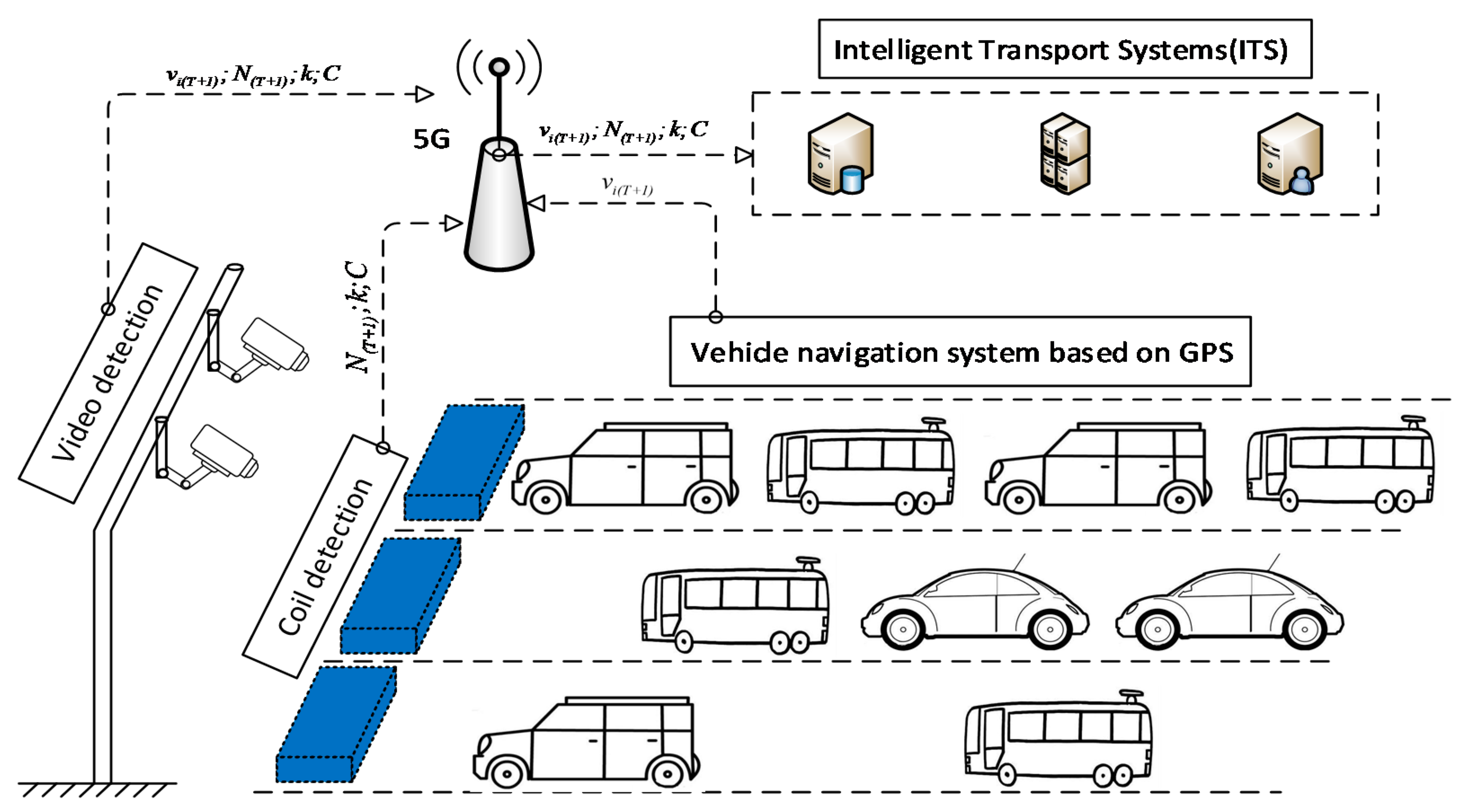
2. Real-Time Traffic Flow Data System and Definitions in 5G-IoV

5G is short for the 5th generation of mobile communication [43,44]. It has the characteristics of a high data rate, reduced delay, energy-savings, increased system capacity, and large-scale device connection, which can improve the performance of the IoV (V2X: vehicle–vehicle interconnection (V2V); vehicle–road interconnection (V2I); vehicle–person interconnection (V2P); vehicle–network interconnection (V2N)), is conducive to the large-scale deployment of IoV environments [45,46,47,48], and provides richer application scenarios for the Internet of Vehicles as well. The deployment of large-scale 5G Internet of Vehicles can provide both real-time multi-sources basic information, such as people, vehicles, roads, and the environment, and a new solution for the acquisition of traffic flow parameters [49,50,51]. Therefore, we defined a real-time traffic flow data system as shown in Figure 1. In this system, each sensor terminal needed to predict the traffic flow parameters it could measure in real time. Vehicles on the road were equipped with GPS car navigation systems that could accurately measure the road location and instantaneous speed of each vehicle in real time. Video detection and loop coil detection could be used to detect the overall situation of traffic on a certain section of the road, which obtained a large amount of traffic flow data including the instantaneous speed of the vehicle, the number of vehicles passing per unit time, the traffic volume monitored per hour, and the number of lanes. The 5G network provided a guarantee for the timely transmission of massive traffic flow data collected through the Internet of Vehicles. These massive flows of traffic data were transmitted to ITS for processing in real time via the 5G network.

Thoroughly considering the advantages and disadvantages of each detection method, the real-time traffic flow data system in 5G-IoV integrates and optimizes the collected and predicted multiple traffic information and extracts reliable and accurate data from it. For example, the instantaneous speed of the vehicle cannot be continuously and accurately extracted and predicted from the monitoring screen through video detection technology in foggy weather, but GPS can make up for it. Moreover, in an environment with a weak GPS signal, video detection technology can be used to obtain, in high-precision, the instantaneous speed of the vehicle. These two technologies combined can accurately obtain the average vehicle speed and its predicted value.

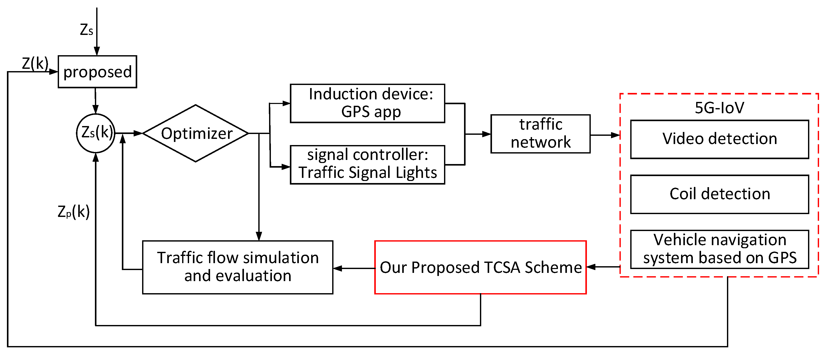
3. Our Proposed TCSA Scheme

The TCSA scheme we proposed predicts traffic flow parameters and obtains the predicted value of the traffic congestion evaluation index through simple calculation and then performs fuzzy comprehensive evaluation. The traffic congestion level under multiple indicators does not have a clear division boundary, which means that it is a fuzzy concept. Therefore, the multi-index fuzzy comprehensive evaluation method can effectively solve this problem. This scheme can help ITS obtain the condition of traffic congestion in advance and provide a basis for decision makers to “actively control” the traffic. The calculation process of the TCSA is shown in Figure 2.

3.1. Selection of Traffic Congestion Evaluation Indicators

Selecting appropriate evaluation indicators can not only improve the accuracy of subsequent traffic congestion situation but also reduce the workload of preliminary data processing. Therefore, the article follows the principles of intuitiveness, sensitivity, convenience, systematicity, independence, and real time to combine the data collected in the 5G-IoV and carefully select the average speed of the road section, traffic flow density, and saturation as evaluation index [19,52].

The average speed refers to the average value of the speeds of all vehicles on the road section within a unit time. This indicator can intuitively reflect the current road traffic congestion. Generally speaking, the higher the speed, the smoother the road; the lower the speed, the more congested the road. It is calculated as follows:

$${\overline{v}}_i=\frac{1}{N}\sum _{i=1}^N{v}_i$$

(1)

where ${\overline{v}}_i$ is the average speed of traffic flow (km/h); $N$ is the number of vehicles passing through the section within a unit time; $v_i$ is the instantaneous speed of the ith vehicle.

Traffic flow density refers to the total number of vehicles per unit length on a lane in a unit time. When there are few vehicles on the road or when the road is stalled due to the fact of congestion, the traffic volume does not change, but the density of traffic varies greatly. Therefore, it plays a decisive role in judging the condition of traffic congestion. The calculation method is as follows:

$$D=\frac{f^{\prime }}{{\overline{v}}_{i}k}$$

(2)

where $D$ is the calculated traffic density (pcu/km); $f^{\prime }$ is the traffic volume monitored per hour (pcu/h); ${\overline{v}}_i$ is the average speed (km/h); k is the number of lanes.

The road section saturation refers to the ratio of the actual traffic volume to the maximum capacity of the road section, which can reflect the actual load of the road. The calculation method is as follows:

$$S=\frac{f}{C}$$

(3)

where $S$ is the road saturation (dimensionless); $f$ is the number of vehicles on each kilometer of roadway (pcu/km); $C$ is the maximum capacity of the road (pcu/km).

3.2. Predicted Value of the Evaluation Index

3.2.1. Traffic Flow Parameter Prediction

The exponential smoothing forecasting method [53] is a simple and easy to implement short-term time-series forecasting method that follows the principle of focusing on the near and overwhelming the far, while taking into account the selected historical data change characteristics. According to the number of smoothing processes, it can be divided into exponential smoothing, quadratic exponential smoothing, and cubic exponential smoothing. When there is no obvious trend change in the data to be predicted, the accuracy of the exponential smoothing is higher; when the data show a certain linear changing trend, the accuracy of the quadratic exponential smoothing method is higher; when the data show a nonlinear trend, the accuracy of the cubic exponential smoothing method is higher. In this paper, assuming that the time series of a parameter is $\left\{x_1,x_2,\dots ,x_3\right\}$, the three exponential smoothing value calculation formula is:

$$\{\begin{array}{c}{S}_t^{\left(1\right)}=\alpha x_t+\left(1-\alpha \right)S_{t-1}^1\hfill \\ S_t^{\left(2\right)}=\alpha S_t^{\left(1\right)}+\left(1-\alpha \right)S_{t-1}^2\\ S_t^{\left(3\right)}=\alpha S_t^{\left(2\right)}+\left(1-\alpha \right)S_{t-1}^3\end{array}$$

(4)

where $S_t^{\left(1\right)}$ is the first smoothing value; $S_t^{\left(2\right)}$ is the second smoothing value; $S_t^{\left(3\right)}$ is the third smoothing value; $\alpha$ is the smoothing coefficient, $\alpha \in \left[0,1\right]$.

Exponential smoothing forecast model:

$$x_{t+1}=S_t^{\left(1\right)}=\alpha {\stackrel{̑}{x}}_t+\left(1-\alpha \right)x_t$$

(5)

Quadratic exponential smoothing forecast model:

$$\{\begin{array}{c}{a}_t=2S_t^{\left(1\right)}-S_t^{\left(2\right)}\hfill \\ b_t=\frac{\alpha }{1-\alpha }(S_t^{\left(1\right)}-S_t^{\left(2\right)})\hfill \\ x_{t+1}=a_t+b_t\hfill \end{array}$$

(6)

Cubic exponential smoothing forecast model:

$$\begin{array}{c}{x}_{\left(t+1\right)}=a_t+b_t+c_t\hfill \\ a_t=3S_t^{\left(1\right)}-3S_t^{\left(2\right)}+S_t^{\left(3\right)}\hfill \\ b_t=\frac{\alpha }{2{(1-\alpha )}^2}[\left(6-5\alpha \right)S_t^{\left(1\right)}-2\left(5-4\alpha \right)S_t^{\left(2\right)}+\left(4-3\alpha \right)S_t^{\left(3\right)}]\hfill \\ c_t=\frac{{\alpha }^2}{2{(1-\alpha )}^2}[S_t^{\left(1\right)}-2S_t^{\left(2\right)}+S_t^{\left(3\right)}]\hfill \end{array}$$

(7)

where $a_t$, $b_t$, and $c_t$ are the model parameters that, respectively, represent the expected value, linear increment, and parabolic increment at time t; $x_t$ is the predicted value of the t period; ${\stackrel{̑}{x}}_t$ is the actual value of the t period.

Considering that the change characteristics in the traffic flow parameters will be affected by holidays, weather, morning and evening peaks, and traffic accidents, the traffic flow parameters are basically stable, change according to a certain rule, and fluctuate irregularly. Therefore, the use of a single exponential smoothing cannot fully adapt to the changing law of traffic flow parameters throughout the forecast period. The change law of traffic flow parameters can be regarded as the accumulation of various changes such as level changes, linear trend changes, nonlinear changes, and periodic changes over time. Therefore, we used DMMAES to forecast, that is, three models were used to predict traffic flow parameters, and the weight of each model was determined through historical data, and the measured value was predicted using the calculated weight and the predicted value of each model.

The DMMAES idea is shown in Figure 3. When predicting the required data, first we calculated the optimal smoothing coefficient of the model based on historical data, and then we performed data predictions separately and adjusted the weight of the model based on the historical data. On this basis, according to the prediction data and weights of each model, the prediction data were fused to obtain the required prediction data. The key of DMMAES is to update the smoothing coefficient and weight of each model.

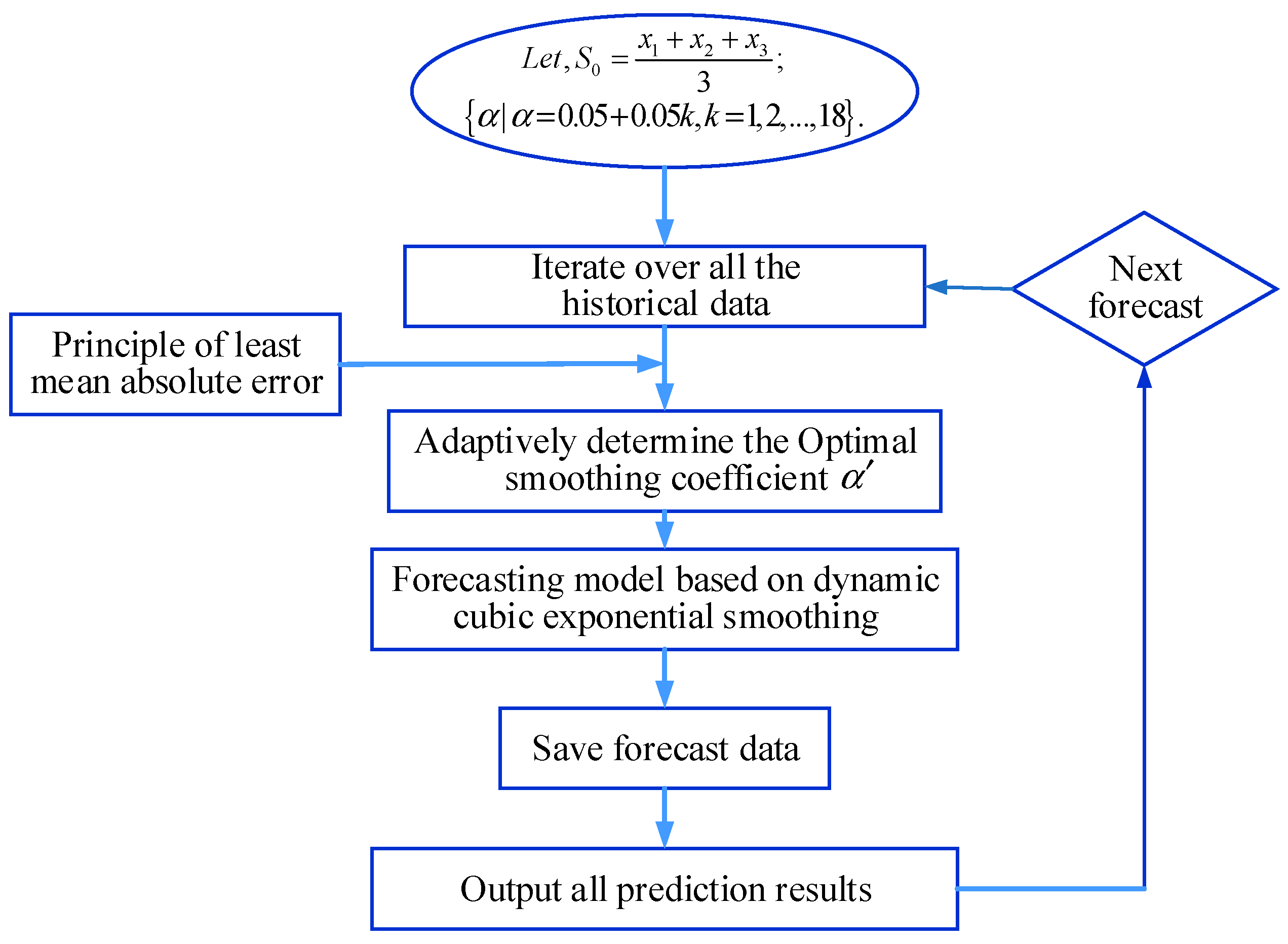
• Optimal smoothing coefficient dynamic calculation method

We proposed an adaptive exponential smoothing and set the sampling period of traffic flow parameters to 6 min, used the latest 10 periods of data as historical data, and the average of the previous three periods of data as the initial smoothing value, and then predicted the traffic flow parameters for the next period, where the smoothing coefficient α could continuously follow-up changes in the historical data and make corresponding adjustments, reducing the impact of changes on objective factors and better follow the principle of minimizing the average absolute error to ensure the accuracy of the prediction results. The calculation process of this method is shown in Figure 4.

ii.

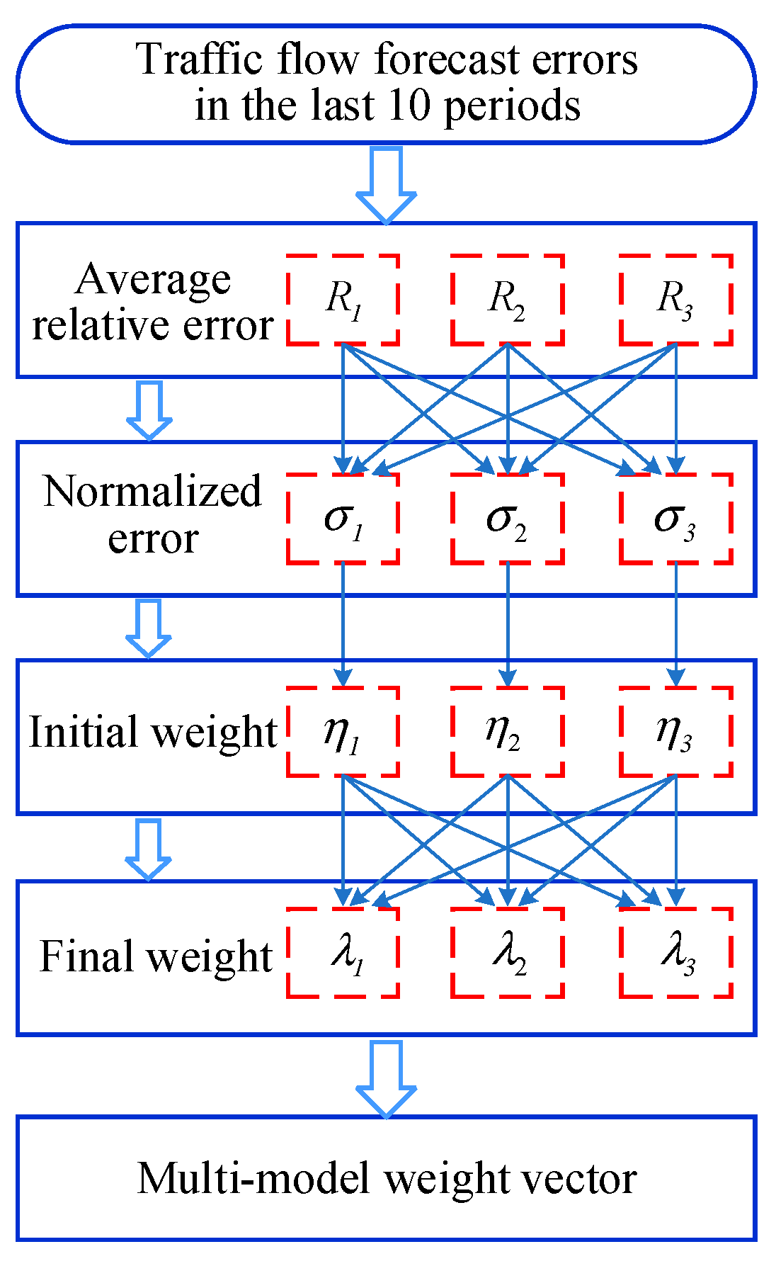
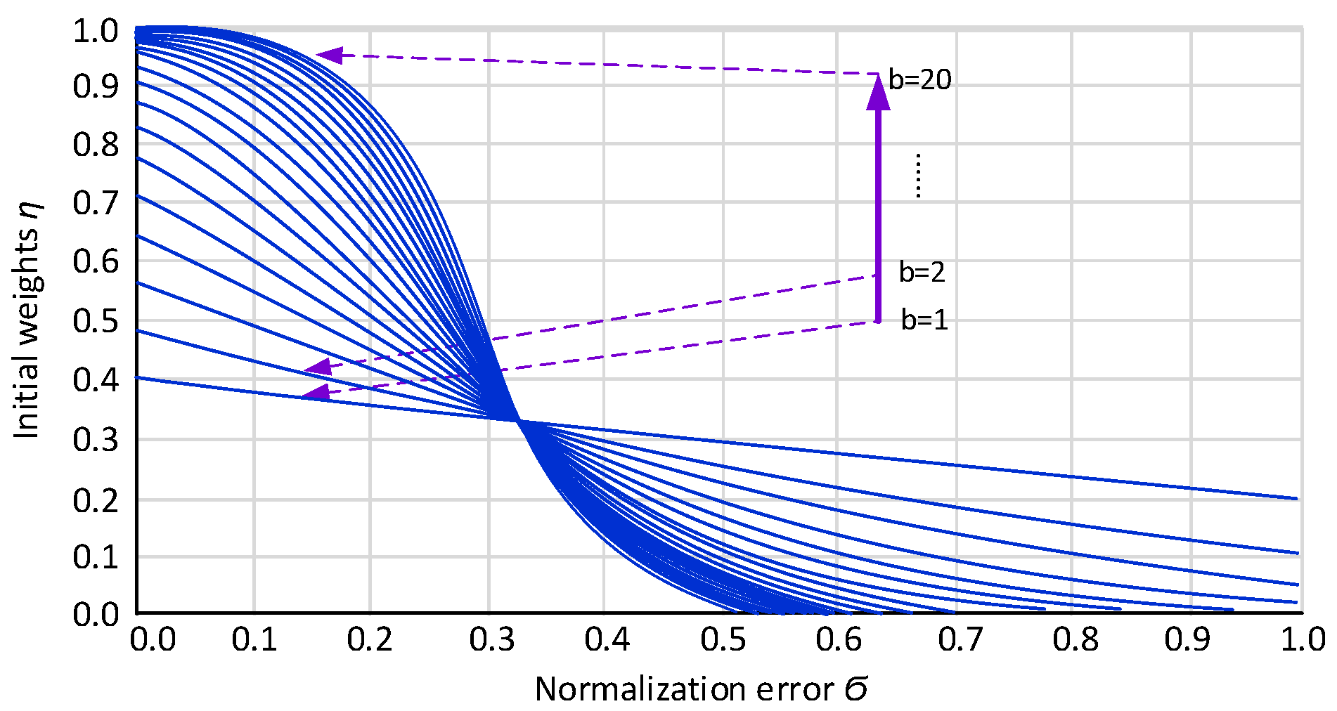
Multi-model weight vector dynamic calculation method

After using the exponential smoothing, quadratic exponential smoothing, and cubic exponential smoothing to predict the measured values that need to be predicted, the data predicted by the three methods needed to be fused by weighted summation. Among them, the weight vector was determined according to the average error of the previous 10 periods of each model. The weight vector determination process is shown in Figure 5.

To calculate the weight vector, the average relative prediction error of the first 10 periods of the three exponential smoothing methods was first calculated, denoted as R₁, R₂, and R₃, and then the average relative error, ${\sigma }_1=R_i/{\sum }^{}{R}_j$, was normalized and, finally, the weight according to the principle that the error was inversely proportional to the weight was determined. Using the sigmoid curve to perform nonlinear processing on the error ensured that the weight difference was not large when the normalization error was small or large at the same time, and that when the normalization error tended to the middle, different errors had a significant impact on the weight.

Assuming that the normalized average relative errors of the three models are ${\sigma }_1$, ${\sigma }_2$, and ${\sigma }_3$, respectively, the model weights are calculated as follows.

Initial weight:

$${\eta }_i=1-\frac{1}{1+a{\mathrm{e}}^{-b{\sigma }_i}}$$

(8)

Final weight:

$${\lambda }_i=\frac{{\eta }_i}{\sum {\eta }_j}$$

(9)

To ensure that the normalization error is 1/3, the step weight is also 1/3, let $a={\mathrm{e}}^{\frac{b}{3}}/2$.

For the determination of b, the difference between the initial weight ${\eta }_i$ and 1 when the normalization error ${\sigma }_i=0$ is as close as possible to the difference between the initial weight ${\eta }_i$ and 0 when the normalization error ${\sigma }_i=1$, while ensuring that the approximate linearity has a sufficiently large variation range. According to the principle of b value selection, the following evaluation function is set:

$$g\left(b\right)=\ln \left({\Delta }_{\sigma }-l_{\sigma }\right)$$

(10)

where ${\Delta }_{\sigma }$ represents the difference between the corresponding initial weight ${\eta }_i$ and 1 or 0 when the normalized error is 0 and 1. $l_{\sigma }$ is the length of the interval, where the difference between the initial weight of the two ends of the interval and the initial weight of the center point does not exceed 10% when the normalized error is taken symmetrically with 1/3 as the center.

When the value of b is 1–20, the relationship between the normalized error and the initial weight is shown in Figure 6.

The variation curve of the evaluation function $g\left(b\right)$ with b is shown in Figure 7. It can be seen that when b = 5, the evaluation function $g\left(b\right)$ takes the minimum value. Therefore, we chose b = 5 as the optimal value of b.

3.2.2. Calculate the Predicted Value of the Evaluation Index

According to Formulas (1) to (3), the predicted values of the traffic congestion evaluation indicators can be calculated from the predicted values of the traffic flow parameters including average traffic flow speed (${\overline{v}}_i$) (km/h), traffic flow density ($D$) (pcu/km/h), and road saturation ($S$).

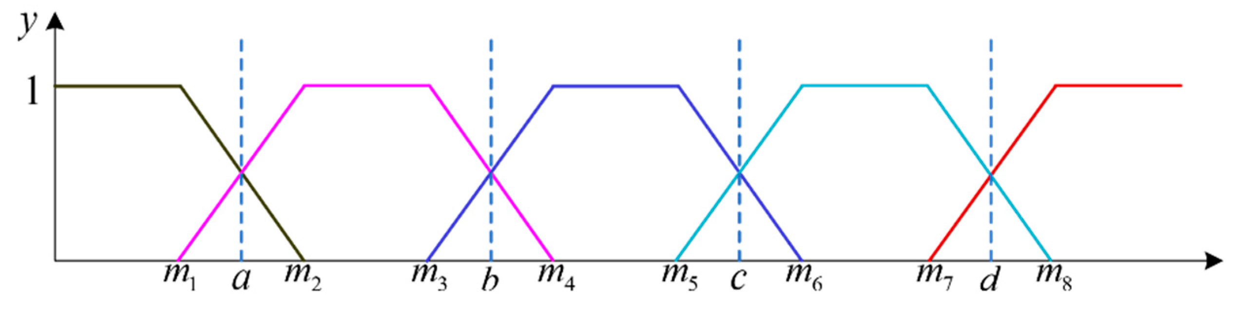
3.3. Select Membership Function

According to the literature [22], congested traffic situations are divided into five levels, and the range of values for the level of traffic congestion corresponding to the three indicators used in this paper is clarified as shown in

Table 2. The value range of the traffic congestion levels of the three indicators.

Indicator Name	Traffic Congestion Levels
	1	2	3	4	5
	Unblocked	Generally Unblocked	Light Congestion	Moderate Congestion	Severe Congestion
${\overline{v}}_i$ (km/h)	(45, $+\infty$)	(35, 45]	(25, 35]	(15, 25]	[0, 15]
D (pcu/km)	(0, 10]	(10, 20]	(20, 30]	(30, 40]	(45, $+\infty$)
S	(0, 0.4]	(0.4, 0.6]	(0.6, 0.8]	(0.8, 1]	(1, +$\infty$)

.

Each indicator corresponds to the corresponding traffic congestion level within a certain range. The closer the indicator value is to the critical value of the range, the lower the degree of membership of the indicator belonging to the corresponding congestion level. Therefore, we adopted the trapezoidal membership function to calculate the membership of the evaluation index belonging to a certain traffic congestion level, where the reduced half trapezoidal membership function and the increased half membership function are used for the two traffic congestion states of unblocked and severely congested traffic, respectively. The membership function graph is shown in Figure 8.

The horizontal axis represents the value of each indicator; a, b, c, and d represent the threshold value of the indicator corresponding to different traffic congestion levels; $m_1,m_2,\dots ,m_8$ represent the linear values of the indicator near the threshold at different traffic congestion levels; the vertical axis is “0” indicates that the corresponding indicator does not belong to a certain traffic congestion level, and “1” means that it meets completely. Since the average speed is a negative indicator, the traffic congestion situations corresponding to their value are severe congestion, moderate congestion, light congestion, generally unobstructed, and unobstructed from left to right. The calculation formula of the membership degree of the traffic congestion evaluation index is as follows.

Level 1:

$$f_1=\{\begin{array}{cc}\hfill 1,\hfill & x\le m_1\hfill \\ \hfill \frac{m_2-x}{m_2-m_1},\hfill & m_1<x<m_2\hfill \\ \hfill 0,\hfill & x\gg m_2\hfill \end{array}$$

(11)

Level 2~4:

$$f_i=\{\begin{array}{cc}\hfill 0,\hfill & x\le m_i\mathrm{or}x\ge m_{i+3}\hfill \\ \hfill \frac{x-m_i}{m_{i+1}-m_i},\hfill & m_i<m_{i+1}\hfill \\ \hfill 1,\hfill & m_{i+1}\le x\le m_{i+2}\hfill \\ \hfill \frac{m_{i+3}-x}{m_{i+3}-m_{i+2}},\hfill & m_{i+2}<x<m_{i+3}\hfill \end{array}, \left(i=2,3,4\right)$$

(12)

Level 5:

$$f_5=\{\begin{array}{cc}\hfill 0,\hfill & x\le m_7\hfill \\ \hfill \frac{x-m_7}{m_8-m_7},\hfill & m_7<x<m_8\hfill \\ \hfill 1,\hfill & x″m_8\hfill \end{array}$$

(13)

According to the membership function, the membership degree l_ij of the jth level of the ith index is obtained, and the membership degree matrix L of the traffic congestion state space can be obtained as shown in Formula (14):

$$L=\left(\begin{array}{c}{L}_1\\ L_2\\ ⋮\\ L_i\end{array}\right)=\left(\begin{array}{cccc}{l}_{11}& l_{12}& \cdots & l_{1j}\\ l_{21}& l_{22}& \cdots & l_{2j}\\ ⋮& ⋮& & ⋮\\ l_{i1}& l_{i2}& \cdots & l_{ij}\end{array}\right)$$

(14)

3.4. Confirming the Weight of the Evaluation Index

The CRITIC method [54] was proposed by Diakoulaki, Mavrotas, and Papayannakis in 1995. We improved the CRITIC method into an adaptive CRITIC method to determine index weight. The adaptive CRITIC can dynamically measure the uncertainty of the indicators and the correlation between indicators based on the indicator data of the last 10 periods. Therefore, using this method to calculate the weights of traffic congestion assessment indicators can more accurately reflect the actual weights of each indicator in different periods. The steps of the adaptive CRITIC method to determine weight are as follows.

Step 1: Process raw data according to Formula (15) to obtain standardized data.

$$K_i=\frac{k_i-k_{imin}}{k_{imax}-k_{imin}}$$

(15)

where $K_i$ is the standardized data of the ith indicator; $k_i$ is the raw data value of the ith indicator; $k_{imax}$ is the maximum value in the raw data of the ith indicator; $k_{imin}$ is the minimum value in the raw data of the ith indicator;

Step 2: Calculate the standard deviation, Si, of the index $k_i$;

Step 3: Calculate the linear correlation coefficient, $R_{i{i}^{\prime }}$, between index, $k_i$, and index, $k_{i^{\prime }}$;

Step 4: Calculate the weight of each indicator according to Formula (16):

$$W_i=\frac{C_i}{{\sum }_{i=1}^g{C}_i}$$

(16)

where $W_i$ is the weight of indicator $k_i$; $C_i=S_i{\sum }_{i^{\prime }=1}^g\left(1-R_{i{i}^{\prime }}\right)$; $i^{\prime }=1,2,\dots ,g$; g is the number of indicators.

3.5. Confirming the Level of Traffic Congestion

The fuzzy comprehensive evaluation matrix was obtained through fuzzy comprehensive evaluation:

$$B=W•L=\left[b_1,b_2,\dots ,b_j\right]$$

(17)

where $W$ is the weight vector of the indicator. According to the principle of maximum membership degree, the level with the maximum membership degree in the fuzzy comprehensive evaluation matrix is selected as the final congestion level. If the maximum value of the final degree of membership is $b_j$, then the traffic congestion level of the traffic sample at this period is $j$.

4. Performance Analysis

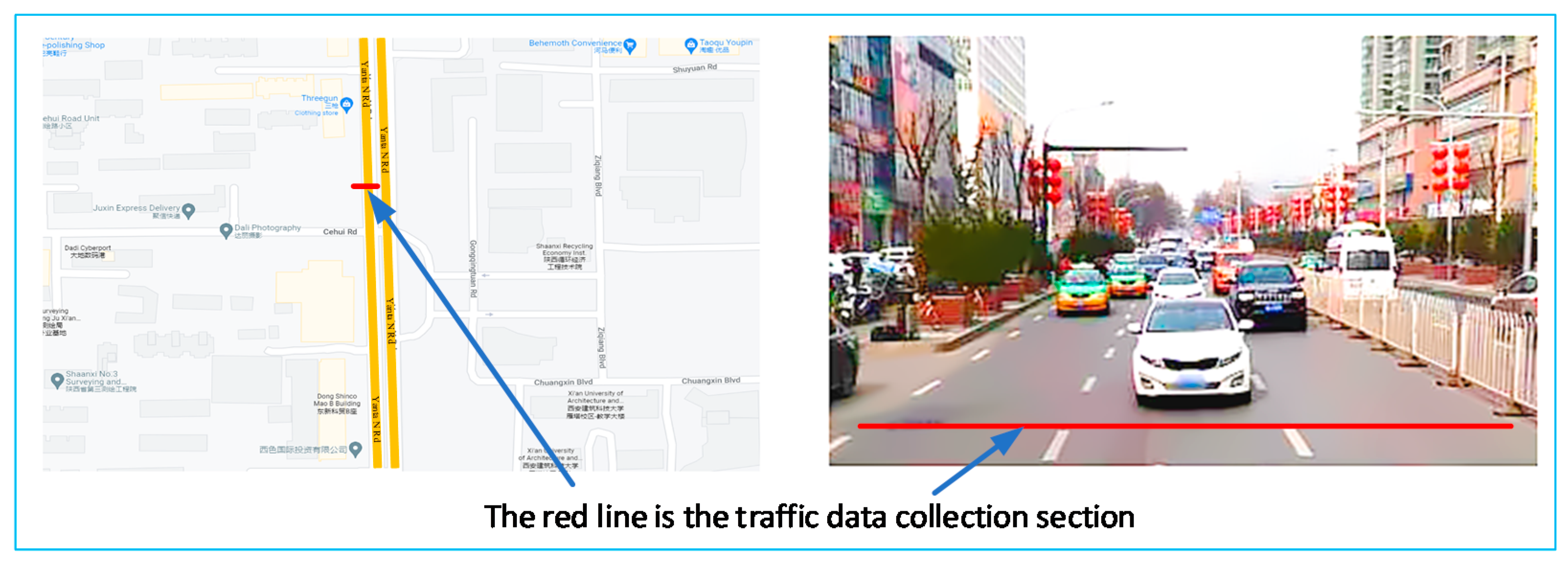
4.1. Data Description

Due to the experimental conditions, it was impossible to collect traffic flow data in a real 5G-IoV environment. The accuracy and reliability of the scheme were tested using traffic flow data of Yanta North Road in Xi’an. Vehicle speed and traffic volume were collected by roadside microwave detectors and video recordings, respectively. It took 6 min of traffic flow data collection to obtain the average vehicle speed and traffic volume. These data sets were analogous to the sequence data obtained after data interaction and processing in the 5G-IoV environment in Figure 1. The data collection range is shown in Figure 9 for three-lane sections traveling from south to north. The collection time was the whole day on 16 October 2019, with a total of 240 data points.

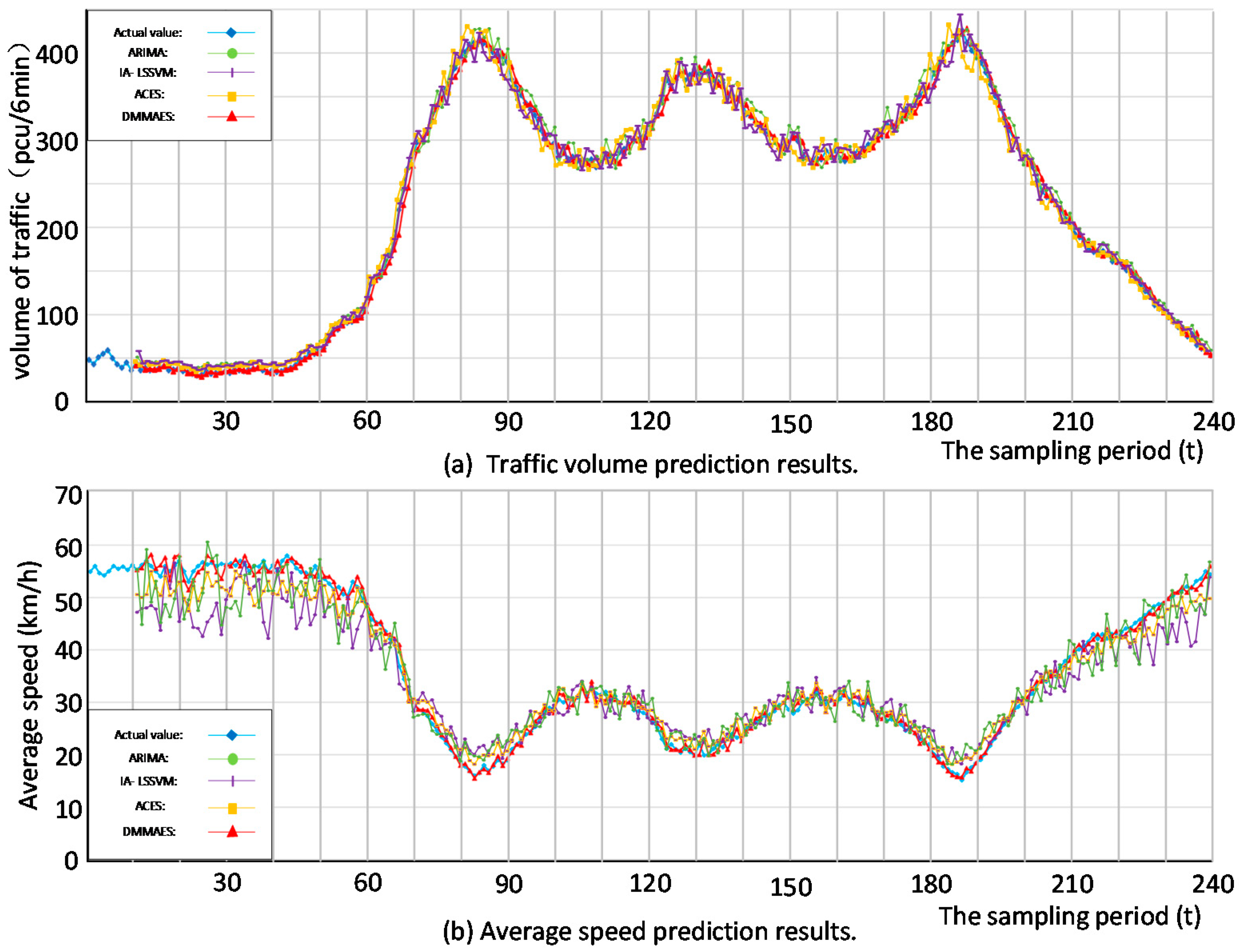
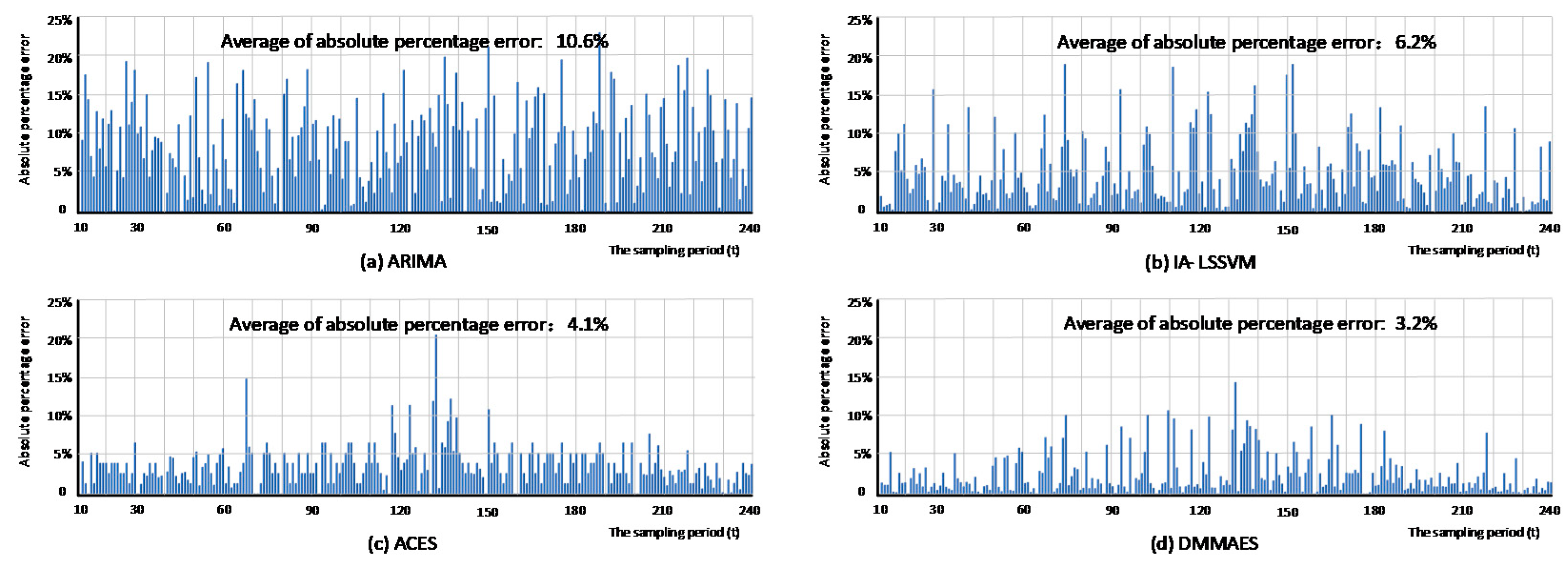
4.2. Predicted Results of Traffic Flow Parameters

The DMMAES was used to realize the one-step, short-term time-series prediction of traffic flow parameters, and the adaptive smoothing coefficient and dynamic multi-model weight vectors were used to improve the prediction accuracy. The next forecast required updating the real-time traffic flow parameters. Assuming that the traffic flow data of the current sampling period are $x_t$, then $\left\{x_{t-9},x_{t-8},\dots ,x_t\right\}$ are historical data, and the exponential smoothing coefficient $\mathsf{\alpha }\prime$ and the multi-model weight vector are dynamically adjusted, and it will predict the traffic flow data $x_{t+1}$ of the next sampling period. In order to verify the effectiveness of the DMMAES prediction algorithm, we used autoregressive integrated moving average (ARIMA), the immune algorithm optimization least squares support vector machine (IA-LSSVM), adaptive cubic exponential smoothing (ACES), and DMMAES to predict traffic volume, $f$, and average speed, ${\overline{v}}_i$. The prediction result is shown in Figure 10.

In order to reflect the accuracy of the prediction results more intuitively, the absolute percentage error was chosen in this paper to reflect the accuracy of the prediction results. The calculation formula is as follows:

$$p_t=\frac{100\left|y_t-{\widehat{y}}_t\right|}{y_t}$$

(18)

where $y_t$ is the actual value; ${\widehat{y}}_t$ is the predicted value; $p_t$ is the absolute percentage error.

The histogram of the absolute percentage error of the traffic volume prediction results corresponding to the four different algorithms is shown in Figure 11, and the corresponding absolute percentage error histogram of the average speed prediction results is shown in Figure 12.

The average absolute percentage error of different prediction algorithms and their computing time are shown in

Table 3. Comparison of prediction errors and the time consumption of the four algorithms.

Data	Prediction Algorithm	ARIMA	IA-LSSVM	ACES	DMMAES
Traffic volume	Average of absolute percentage error	7.3%	4.8%	3.6%	2.7%
	Time consuming (s)	0.83	38.15	0.32	0.62
Average speed	Average of absolute percentage error	10.6%	6.2%	4.1%	3.2%
	Time consuming (s)	0.81	36.26	0.26	0.51

. The operating environment of the algorithm is Windows 10 system, the processor was an Intel Core [email protected] Hz, and the memory was 16 G.

The experimental results showed that our proposed DMMAES could predict traffic flow parameters well. Through horizontal comparison, it can be seen that the absolute percentage error of the prediction results using DMMAES was better than other algorithms. This was because there were many changing trends in the traffic flow parameters, and DMMAES could better adapt to the changing law of traffic flow parameters, thereby reducing the prediction error. In addition, compared with the artificial intelligence algorithm IA-LSSTM, DMMAES has a simple structure and has a much lower computational complexity than IA-LSSTM and consumes much less time than IA-LSSTM, making it suitable for 5G-LOV prediction of traffic flow parameters on the sensor side.

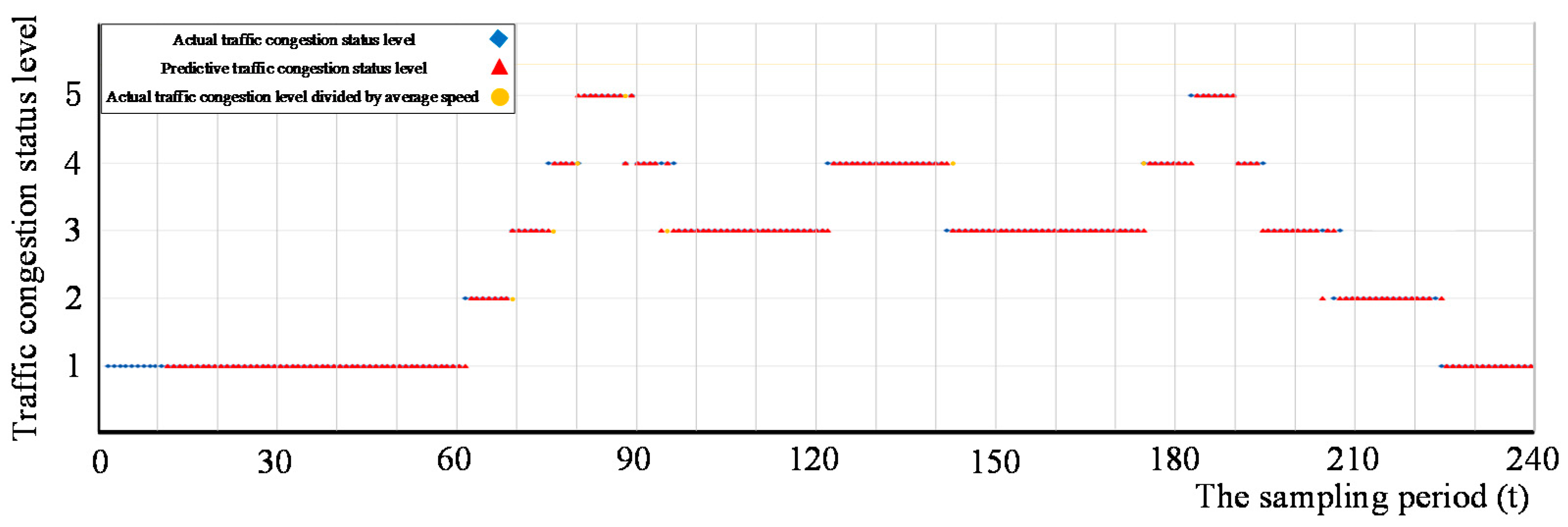
4.3. Predicted Results of Traffic Congestion Level

According to the predicted results of the average speed, ${\overline{v}}_{i_{(t+1)}},$ and traffic volume, $f_{t+1}$, in period t + 1, the traffic flow density, D_t+1, and saturation, S_t+1, in period t + 1 were calculated according to Formulas (2) and (3), where the number of lanes on the road was three, and the road design had a maximum traffic capacity of 3800 pcu/h.

After determining the divided trapezoidal membership function, according to the value range of the traffic congestion evaluation index shown in Table 1, and calculating the membership matrix, L_t+1, of the traffic congestion evaluation index for the period t + 1, we used the last 10 periods of the traffic congestion evaluation index values as the raw data and the adaptive CRITIC method to calculate the weight, w_i, of each index in the t + 1 period to obtain the weight vector, W_t+1. Figure 13 shows that the weights we calculated can objectively reflect the impact of different indicators on traffic congestion at different time periods.

Then, the membership degree of each traffic congestion level was calculated by Formula (17) and, finally, the traffic congestion level of the period t + 1 was determined according to the principle of the maximum membership degree. Figure 14 shows the comparison between the predicted value of traffic congestion and the actual one. There were 230 traffic congestion level prediction data points, of which only seven data points were inconsistent with the actual traffic congestion level, and 10 data points were different from level evaluated only by the average speed.

4.4. Application of the TCSA Scheme in Traffic Management

The agglomeration effect of cities has led to increasing pressure on urban traffic operations, and the problem of traffic congestion has seriously restricted the development of towns, especially during peak hours. If scientific and reasonable traffic management is not carried out, the entire road network will be partially congested, and resources will be wasted. In our defined 5G-IoV real-time traffic flow data system, each sensor terminal, such as a vehicle navigation system, coil detection, and video vehicle detection, can detect traffic flow parameters in real time under suitable conditions. The detection and prediction data of each terminal can be fused with each other to improve the detection and prediction accuracy of its traffic flow parameters. Due to the consideration of construction costs, the hardware configuration of the above sensor terminal was not high. We designed a TCSA scheme with low hardware requirements, fast calculation speed, and high precision.

Based on the classic traffic guidance control system [55,56], we embedded the TCSA scheme in it. As shown in Figure 15, the structure diagram of the traffic guidance control system improved by the TCSA scheme. In the traffic flow information processing link, the TCSA scheme was used to provide the relevant performance indicators Zp(k) of each road segment in the prediction time domain, such as traffic flow density, road saturation, average vehicle speed, and road congestion level. Through the performance index Z(k) of the current road network traffic flow and the proposed value Zs, the future performance index Zs(k) was determined according to the TCSA module, the traffic flow simulation and evaluation module, and the optimal control input in the system. Through the function of the optimizer, the performance index Zp(k) was close to the proposed performance index Zs(k) so as to realize the output solution of the controller.

The result of the traffic guidance control is realized by the traffic management center in the ITS through the traffic control guidance system to control the time of the signal lights of the city intersection. It shares information with other subsystems through the traffic information center, and the subsystem provides detailed traffic information for the traffic management center. For example, the GPS navigation system provides a traveler with a time-optimized or distance-optimized travel path according to the results of traffic guidance control and the collected vehicle positioning information. The above methods can improve the operation efficiency of the urban road network and alleviate the problem of urban traffic congestion.

5. Conclusions and Future Work

As the front end of the intelligent transportation system, 5G-IoV is used to collect and transmit massive traffic flow data in real-time to ensure the real-time and high efficiency of traffic management. Our research provides a comprehensive solution scheme for the prediction and evaluation of traffic congestion in the 5G-IoV environments. The experimental results show that the TCSA scheme proposed in this paper can accurately predict and evaluate the level of traffic congestion based on real-time traffic flow data, which benefits from the following innovations:

(1)

The DMMAES prediction algorithm can dynamically adjust the smoothing coefficient and weight of the model according to the changing trend of traffic flow parameters;

(2)

The membership degree of the traffic congestion index was calculated using the trapezoidal membership function. The boundaries among the various thresholds that conform to the traffic congestion state was not clear, and there was ambiguity;

(3)

The adaptive CRITIC method was used to determine the weights of traffic congestion evaluation indicators, which can reflect not only the conflict between the indicators, but also the impact of the indicators on the traffic congestion in different periods.

However, the reasons that affect the accuracy of traffic congestion prediction are very complicated. Within the framework of our proposed traffic congestion assessment plan, there are still some areas that can be improved. In order to develop a more effective traffic management plan, it is necessary to appropriately increase the traffic congestion prediction step size, and at the same time, appropriate traffic congestion indicators should be selected to improve the prediction accuracy. In future work, we will focus on the following challenges:

(1)

Enhance 5G-IoV perception capabilities, such as the ability to perceive weather changes and traffic accidents;

(2)

Increase the traffic flow prediction step size without reducing the prediction accuracy;

(3)

Add new traffic congestion evaluation indicators and propose corresponding weight calculation methods. Next, we will consider the impact of weather conditions and the service level of public transportation near roads on traffic congestion and try to develop a combination of a subjective and objective weighting method to determine the index weight.

References

1. Chow, A.H.; Santacreu, A.; Tsapakis, I.; Tanasaranond, G.; Cheng, T. Empirical assessment of urban traffic congestion. J. Adv. Transp. 2014, 48, 1000–1016. [Google Scholar] [CrossRef] [Green Version]
2. Knorr, F.; Baselt, D.; Schreckenberg, M.; Mauve, M. Reducing traffic jams via VANETs. IEEE Trans. Veh. Technol. 2012, 61, 3490–3498. [Google Scholar] [CrossRef]
3. Wu, F.; Stern, R.E.; Cui, S.; Delle Monache, M.L.; Bhadani, R.; Bunting, M.; Miles, C.; Nathaniel, H.; R’mani, H.; Benedetto, P.; et al. Tracking vehicle trajectories and fuel rates in phantom traffic jams: Methodology and data. Transp. Res. Part C Emerg. Technol. 2019, 99, 82–109. [Google Scholar] [CrossRef] [Green Version]
4. Fabre, M.; Faure, S.; Laurière, M.; Maury, B.; Perrin, C. Non classical solution of a conservation law arising in vehicular traffic modelling. ESAIM Proc. Surv. 2016, 55, 131–147. [Google Scholar] [CrossRef] [Green Version]
5. Sjoberg, K.; Andres, P.; Buburuzan, T.; Brakemeier, A. Cooperative intelligent transport systems in Europe: Current deployment status and outlook. IEEE Veh. Technol. Mag. 2017, 12, 89–97. [Google Scholar] [CrossRef]
6. Yin, J.; Lo, W.; Deng, S.; Li, Y.; Wu, Z.; Xiong, N. Colbar: A collaborative location-based regularization framework for QoS prediction. Inf. Sci. 2014, 265, 68–84. [Google Scholar] [CrossRef]
7. Kumar, P.M.; Manogaran, G.; Sundarasekar, R.; Chilamkurti, N.; Varatharajan, R. Ant colony optimization algorithm with internet of vehicles for intelligent traffic control system. Comput. Netw. 2018, 144, 154–162. [Google Scholar] [CrossRef]
8. Zhang, Q.; Zhou, C.; Tian, Y.C.; Xiong, N.; Qin, Y.; Hu, B. A fuzzy probability Bayesian network approach for dynamic cybersecurity risk assessment in industrial control systems. IEEE Trans. Ind. Inform. 2017, 14, 2497–2506. [Google Scholar] [CrossRef] [Green Version]
9. Sharif, A.; Li, J.P.; Saleem, M.A. Internet of things enabled vehicular and ad hoc networks for smart city traffic monitoring and controlling: A review. Int. J. Adv. Netw. Appl. 2018, 10, 3833–3842. [Google Scholar] [CrossRef]
10. Guo, W.; Xiong, N.; Vasilakos, A.V.; Chen, G.; Cheng, H. Multi-source temporal data aggregation in wireless sensor networks. Wirel. Pers. Commun. 2011, 56, 359–370. [Google Scholar] [CrossRef]
11. Ray, P.P. A survey on Internet of Things architectures. J. King Saud Univ.-Comput. Inf. Sci. 2018, 30, 291–319. [Google Scholar]
12. Chen, M.; Tian, Y.; Fortino, G.; Zhang, J.; Humar, I. Cognitive internet of vehicles. Comput. Commun. 2018, 120, 58–70. [Google Scholar] [CrossRef]
13. Xu, W.; Zhou, H.; Cheng, N.; Lyu, F.; Shi, W.; Chen, J.; Shen, X. Internet of vehicles in big data era. IEEE/CAA J. Autom. Sin. 2018, 5, 19–35. [Google Scholar] [CrossRef]
14. Shankar, H.; Raju, P.L.N.; Rao, K.R.M. Multi model criteria for the estimation of road traffic congestion from traffic flow information based on fuzzy logic. J. Transp. Technol. 2012, 2, 50. [Google Scholar] [CrossRef] [Green Version]
15. Li, S.; Da Xu, L.; Zhao, S. 5G Internet of Things: A survey. J. Ind. Inf. Integr. 2018, 10, 1–9. [Google Scholar] [CrossRef]
16. Duan, W.; Gu, J.; Wen, M.; Zhang, G.; Ji, Y.; Mumtaz, S. Emerging Technologies for 5G-IoV Networks: Applications, Trends and Opportunities. IEEE Netw. 2020, 34, 283–289. [Google Scholar] [CrossRef]
17. Wang, Z.; Li, T.; Xiong, N.; Pan, Y. A novel dynamic network data replication scheme based on historical access record and proactive deletion. J. Supercomput. 2012, 62, 227–250. [Google Scholar] [CrossRef]
18. Ahmad, M.; Chen, Q.; Khan, Z. Microscopic Congestion Detection Protocol in VANETs. J. Adv. Transp. 2018, 2018, 6387063. [Google Scholar] [CrossRef]
19. Rao, A.M.; Rao, K.R. Measuring urban traffic congestion-a review. Int. J. Traffic Transp. Eng. 2012, 2, 286–305. [Google Scholar]
20. Lu, Y.; Wu, S.; Fang, Z.; Xiong, N.; Yoon, S.; Park, D.S. Exploring finger vein based personal authentication for secure IoT. Future Gener. Comput. Syst. 2017, 77, 149–160. [Google Scholar] [CrossRef]
21. Yao, Y.; Xiong, N.; Park, J.H.; Ma, L.; Liu, J. Privacy-preserving max/min query in two-tiered wireless sensor networks. Comput. Math. Appl. 2013, 65, 1318–1325. [Google Scholar] [CrossRef]
22. Chen, Y.; Chen, C.; Wu, Q.; Ma, J.; Zhang, G.; Milton, J. Spatial-temporal traffic congestion identification and correlation extraction using floating car data. J. Intell. Transp. Syst. 2020, 25, 263–280. [Google Scholar] [CrossRef]
23. He, F.; Yan, X.; Liu, Y.; Ma, L. A traffic congestion assessment method for urban road networks based on speed performance index. Procedia Eng. 2016, 137, 425–433. [Google Scholar] [CrossRef] [Green Version]
24. Yang, P.; Xiong, N.; Ren, J. Data security and privacy protection for cloud storage: A survey. IEEE Access 2020, 8, 131723–131740. [Google Scholar] [CrossRef]
25. Smilowitz, K.R.; Daganzo, C.F. Reproducible features of congested highway traffic. Math. Comput. Model. 2002, 35, 509–515. [Google Scholar] [CrossRef]
26. Zhou, Z.; Zhao, Q.P. Study on RTI congestion control based on the layer of interest. J. Softw. 2004, 15, 120–130. [Google Scholar]
27. Gore, R.; Kamensky, D.; Diallo, S.; Padilla, J. Statistical debugging for simulations. ACM Trans. Modeling Comput. Simul. (TOMACS) 2015, 25, 1–26. [Google Scholar] [CrossRef]
28. Kamensky, D.; Gore, R.; Reynolds, P.F. Applying enhanced fault localization technology to Monte Carlo simulations. In Proceedings of the 2011 Winter Simulation Conference (WSC), Phoenix, AZ, USA, 11–14 December 2011; pp. 2798–2809. [Google Scholar]
29. Altunkaynak, A.; Özger, M.; Çakmakci, M. Water consumption prediction of Istanbul city by using fuzzy logic approach. Water Resour. Manag. 2005, 19, 641–654. [Google Scholar] [CrossRef]
30. Akkurt, S.; Tayfur, G.; Can, S. Fuzzy logic model for the prediction of cement compressive strength. Cem. Concr. Res. 2004, 34, 1429–1433. [Google Scholar] [CrossRef] [Green Version]
31. Qu, Y.; Xiong, N.N. RFH: A resilient, fault-tolerant and high-efficient replication algorithm for distributed cloud storage. In Proceedings of the 41st International Conference on Parallel Processing, Pittsburgh, PA, USA, 10–13 September 2012; pp. 520–529. [Google Scholar]
32. Habtemichael, F.G.; Cetin, M. Short-term traffic flow rate forecasting based on identifying similar traffic patterns. Transp. Res. Part C Emerg. Technol. 2016, 66, 61–78. [Google Scholar] [CrossRef]
33. Qi, S.; Jiang, D.; Huo, L. A Prediction Approach to End-to-End Traffic in Space Information Networks. Mob. Netw. Appl. 2019, 26, 726–735. [Google Scholar] [CrossRef]
34. Luo, X.; Li, D.; Yang, Y.; Zhang, S. Spatiotemporal traffic flow prediction with KNN and LSTM. J. Adv. Transp. 2019, 2019, 4145353. [Google Scholar] [CrossRef] [Green Version]
35. Shen, M.; Wei, M.; Zhu, L.; Wang, M. Classification of encrypted traffic with second-order markov chains and application attribute bigrams. IEEE Trans. Inf. Forensics Secur. 2017, 12, 1830–1843. [Google Scholar] [CrossRef]
36. Xu, D.; Wei, C.; Peng, P.; Xuan, Q.; Guo, H. GE-GAN: A novel deep learning framework for road traffic state estimation. Transp. Res. Part C Emerg. Technol. 2020, 117, 102635. [Google Scholar] [CrossRef]
37. Kadkhodaei, M.; Shad, R. Analysis and Evaluation of Traffic Congestion Control Methods in Touristic Metropolis Using Analytical Hierarchy Process (AHP). Civ. Eng. J. 2018, 4, 602–608. [Google Scholar] [CrossRef]
38. Wan, R.; Xiong, N. An energy-efficient sleep scheduling mechanism with similarity measure for wireless sensor networks. Hum.-Cent. Comput. Inf. Sci. 2018, 8, 1–22. [Google Scholar] [CrossRef] [Green Version]
39. Berrouk, S.; Fazziki, A.E.; Sadgal, M. Fuzzy-Based Approach for Assessing Traffic Congestion in Urban Areas. Int. Conf. Image Signal Process. 2020, 12119, 112–121. [Google Scholar]
40. Kong, X.; Xu, Z.; Shen, G.; Wang, J.; Yang, Q.; Zhang, B. Urban traffic congestion estimation and prediction based on floating car trajectory data. Future Gener. Comput. Syst. 2016, 61, 97–107. [Google Scholar] [CrossRef]
41. Wan, Z.; Xiong, N.; Ghani, N.; Vasilakos, A.V.; Zhou, L. Adaptive unequal protection for wireless video transmission over IEEE 802.11 e networks. Multimed. Tools Appl. 2014, 72, 541–571. [Google Scholar] [CrossRef]
42. Ermagun, A.; Levinson, D. Spatiotemporal traffic forecasting: Review and proposed directions. Transp. Rev. 2018, 38, 786–814. [Google Scholar] [CrossRef]
43. He, R.; Xiong, N.; Yang, L.T.; Park, J.H. Using multi-modal semantic association rules to fuse keywords and visual features automatically for web image retrieval. Inf. Fusion 2011, 12, 223–230. [Google Scholar] [CrossRef]
44. Shafi, M.; Molisch, A.F.; Smith, P.; Haustein, T.; Zhu, P.; De Silva, P.; Tufvesson, F.; Benjebbour, A.; Wunder, G. 5G: A tutorial overview of standards, trials, challenges, deployment, and practice. IEEE J. Sel. Areas Commun. 2017, 35, 1201–1221. [Google Scholar] [CrossRef]
45. Wu, M.; Tan, L.; Xiong, N. A structure fidelity approach for big data collection in wireless sensor networks. Sensors 2015, 15, 248–273. [Google Scholar] [CrossRef] [PubMed] [Green Version]
46. Huang, S.; Liu, A.; Wang, T.; Xiong, N.N. BD-VTE: A novel baseline data based verifiable trust evaluation scheme for smart network systems. IEEE Trans. Netw. Sci. Eng. 2020, 8, 2087–2105. [Google Scholar] [CrossRef]
47. Li, H.; Liu, J.; Wu, K.; Yang, Z.; Liu, R.W.; Xiong, N. Spatio-temporal vessel trajectory clustering based on data mapping and density. IEEE Access 2018, 6, 58939–58954. [Google Scholar] [CrossRef]
48. Kombate, D. The Internet of Vehicles based on 5G communications. In Proceedings of the 2016 IEEE International Conference on Internet of Things (iThings) and IEEE Green Computing and Communications (GreenCom) and IEEE Cyber, Physical and Social Computing (CPSCom) and IEEE Smart Data (SmartData), Chengdu, China, 15–18 December 2016; pp. 445–448. [Google Scholar]
49. Xia, F.; Hao, R.; Li, J.; Xiong, N.; Yang, L.T.; Zhang, Y. Adaptive GTS allocation in IEEE 802.15. 4 for real-time wireless sensor networks. J. Syst. Archit. 2013, 59, 1231–1242. [Google Scholar] [CrossRef]
50. Yang, X.; Luo, S.; Gao, K.; Qiao, T.; Chen, X. Application of data science technologies in intelligent prediction of traffic congestion. J. Adv. Transp. 2019, 2019, 2915369. [Google Scholar] [CrossRef] [Green Version]
51. Gao, K.; Han, F.; Dong, P.; Xiong, N.; Du, R. Connected vehicle as a mobile sensor for real time queue length at signalized intersections. Sensors 2019, 19, 2059. [Google Scholar] [CrossRef] [Green Version]
52. Rui, L.; Zhang, Y.; Huang, H.; Qiu, X. A New Traffic Congestion Detection and Quantification Method Based on Comprehensive Fuzzy Assessment in VANET. KSII Trans. Internet Inf. Syst. 2018, 12, 41–60. [Google Scholar]
53. Jiang, Y.; Tong, G.; Yin, H.; Xiong, N. A pedestrian detection method based on genetic algorithm for optimize XGBoost training parameters. IEEE Access 2019, 7, 118310–118321. [Google Scholar] [CrossRef]
54. Diakoulaki, D.; Mavrotas, G.; Papayannakis, L. Determining objective weights in multiple criteria problems: The critic method. Comput. Oper. Res. 1995, 22, 763–770. [Google Scholar] [CrossRef]
55. Lin, C.; He, Y.X.; Xiong, N. An energy-efficient dynamic power management in wireless sensor networks. In Proceedings of the 2006 Fifth International Symposium on Parallel and Distributed Computing, Timisoara, Romania, 6–9 July 2006; Volume 2006, pp. 148–154. [Google Scholar]
56. Jia, D.; Chen, H.; Zheng, Z.; Watling, D.; Connors, R.; Gao, J.; Li, Y. An enhanced predictive cruise control system design with data-driven traffic prediction. IEEE Trans. Intell. Transp. Syst. 2021, 2021, 1–14. [Google Scholar] [CrossRef]
Figure 1. Real-time traffic flow data system in 5G-IoV.
Electronics 11 01032 g001
Figure 2. Traffic congestion situation assessment (TCSA) scheme.
Electronics 11 01032 g002
Figure 3. Algorithm concept of dynamic multi-model adaptive exponential smoothing (DMMAES).
Electronics 11 01032 g003
Figure 4. The calculation process of the adaptive exponential smoothing.
Electronics 11 01032 g004
Figure 5. The calculation process of the multi-model weight vector.
Electronics 11 01032 g005
Figure 6. The relationship between normalized error and initial weight for different b values.
Electronics 11 01032 g006
Figure 7. The relationship between the evaluation function g ( b ) and the b value.
Electronics 11 01032 g007
Figure 8. Trapezoidal membership function of traffic congestion levels.
Electronics 11 01032 g008
Figure 9. Scope of traffic flow data collection.
Electronics 11 01032 g009
Figure 10. Traffic volume, f , and average speed, v ¯ i , prediction results.
Electronics 11 01032 g010
Figure 11. Histogram of the absolute percentage error of traffic volume prediction results.
Electronics 11 01032 g011
Figure 12. Histogram of the absolute percentage error of the average speed prediction results.
Electronics 11 01032 g012
Figure 13. Weight of the traffic congestion evaluation index.
Electronics 11 01032 g013
Figure 14. Predicted traffic congestion level and actual traffic congestion level.
Electronics 11 01032 g014
Figure 15. Structure diagram of the improved traffic guidance control system based on the TCSA scheme.
Electronics 11 01032 g015