Efficient Wind Power Prediction Using Machine Learning Methods: A Comparative Study

Abstract

Wind power represents a promising source of renewable energies. Precise forecasting of wind power generation is crucial to mitigate the challenges of balancing supply and demand in the smart grid. Nevertheless, the major difficulty in wind power is its high fluctuation and intermittent nature, making it challenging to forecast. This study aims to develop efficient data-driven models to accurately forecast wind power generation. Crucially, the main contributions of this work are listed in the following major elements. Firstly, we investigate the performance of enhanced machine learning models to forecast univariate wind power time-series data. Specifically, we employed Bayesian optimization (BO) to optimally tune hyperparameters of the Gaussian process regression (GPR), Support Vector Regression (SVR) with different kernels, and ensemble learning (ES) models (i.e., Boosted trees and Bagged trees) and investigated their forecasting performance. Secondly, dynamic information has been incorporated in their construction to further enhance the forecasting performance of the investigated models. Specifically, we introduce lagged measurements to enable capturing time evolution into the design of the considered models. Furthermore, more input variables (e.g., wind speed and wind direction) are used to further improve wind prediction performance. Actual measurements from three wind turbines in France, Turkey, and Kaggle are used to verify the efficiency of the considered models. The results reveal the benefit of considering lagged data and input variables to better forecast wind power. The results also showed that the optimized GPR and ensemble models outperformed the other machine learning models.

1. Introduction

Wind power capacity has shown a rapid increase recently and has become a promising source of renewable energies. For instance, 8.4% of the total U.S. utility-scale electricity generation is provided by wind turbines in 2020, and it is expected to reach 20% by 2030 and 35% by 2050 [1]. The significant advantage of wind energy is avoiding approximately 189 million metric tons of CO${}_2$ emissions and reducing water usage by about 103 billion gallons compared to traditional power sources [1]. However, the main challenges in wind power management reside in its intermittent fluctuations mainly due to weather conditions, which makes its integration into a power grid a challenging task [2]. Thus, predicting wind power is undoubtedly necessary for the efficient integration of wind turbines into the power grid.

Over the last two decades, there has been increasing interest in developing accurate wind power prediction methods [3,4]. Two main types of models can be distinguished: physical-based and data-driven models [5]. Physical models employed atmospheric motion equations for estimating the evolution of meteorological measurements, and then they used the estimated meteorological variables for wind power prediction [6]. Essentially, predicting wind power via a physical model using numerical weather estimation is accomplished in two phases: at first, wind speed is predicted and then transformed into wind power [7]. However, physical models are generally costly and time-consuming to design, producing low prediction precision for a local area [8]. In contrast to physical approaches based on very complex differential equations, the data-based models derive functional dependencies directly from the data to build a model that describes the relations between wind power and other input variables [9,10].

Efficiently predicting wind power is vital to help operators integrate wind turbines in smart-grids and improve the management of power output. Various data-driven approaches have been developed in the literature to improve wind power prediction. Traditional time-series methods, including the autoregressive moving average (ARMA) model and its variants, have been widely used for short-term wind power forecasting [11,12]. The method in [13] used an ARMA model to forecast hourly wind power. It showed good forecasting performance for one hour ahead and declines in precision further along in time. These models are simple to construct and convenient to implement. However, it is worthwhile noticing that traditional time-series models (e.g., ARMA and its variants) can reach a satisfying performance when wind power data show regular variations, but the forecast error is obvious when the wind power time series shows irregular variations. In [14], a coupled strategy integrating ARMA and an artificial neural network (ANN) has been proposed to short-term forecast wind power. This study showed that the coupled approach provided a better forecasting performance compared to the standalone ARMA and ANN.

Various machine learning methods have been developed in the literature to predict wind power in recent decades. In [15], Bhaskar and Singh conducted a two-stage approach to improve wind power forecasting. At first, after the decomposition of wind time-series using wavelet decomposition, an adaptive wavelet neural network (AWNN) approach is applied for regression of every decomposed signal 30 h ahead of predicting the wind speed. Then, a feed-forward neural network is employed to establish the mapping between wind speed and wind power output. The latter enables transforming the forecasted wind speed into wind power prediction. They showed that the AWNN approach offers the best approximation and fast training capacity in comparison to a feed-forward neural network (FFNN). Chen et al. proposed a wind power forecasting approach based on Gaussian processes and numerical weather prediction [16]. Azimi et al. considered the K-means clustering method combined with a cluster selection algorithm for better extracting features from wind time-series data [17]. Then, a hybrid wind power forecaster is proposed using data mining, discrete wavelet transform, and a multilayer perceptron neural network. They highlighted that cluster selection makes the forecast process faster since only the relevant portion of data is used to train the forecaster rather than using the whole dataset. Further, Yang et al. proposed a support-vector-machine (SVM)-enhanced Markov method for short-term wind power forecasting [18]. Specifically, the data analytic-based finite-state Markov procedures are first performed to model the nominal evolution of wind generation. Then, the forecast using SVM is merged appropriately into the finite-state Markov models. The study in [19] showed that an artificial neural network (ANN) model reasonably predicted wind power and outperformed analytical models due to its flexibility and ability to model process nonlinearity. The method in [20] combines the benefits of the wavelet transform and neural networks with tapped delay to forecast wind power. However, it is worthwhile to notice that this approach cannot be performed online because the wavelet transform requires batch data. In [21], an approach based on sparse vector autoregression is introduced for very short-term probabilistic wind power forecasting. Wu et al. used a mean trend detector (MTD) and a mathematical morphology-based local predictor (MMLP) for multistep-ahead forecasting of wind power generation [22]. Demolli et al. proposed wind power forecasting using machine learning algorithms [23]. Specifically, they applied random forest regression (RF), support vector regression (SVR), k-nearest neighbors (kNN), and least absolute shrinkage and selection operator (LASSO) regression to forecast the wind power based on historical daily wind speed data. They highlight that machine learning models could be used to a location distinct from model-trained locations. However, these models are static and ignore information in past data. Importantly, when the temporal dependence in time-series data is moderate or high, considering time-lagged values could improve forecast accuracy. Several data-driven methods developed in the literature, such as lagged-ensemble machine learning [24,25] and dynamic principal component regression [26], demonstrated the potential improvement of forecast accuracy using lagged data when compared with the static counterpart.

In addition, various machine learning techniques have been developed in the literature by merging the advantages of different models to further improve their prediction accuracy. For instance, Liu et el. proposed a hybrid approach based on an orthogonal test and SVM (OT-SVM) to forecast the wind power ramp [27]. They achieved better prediction precision compared to Spearman-SVM, Grey Correlation Degree-SVM, and principal components analysis-SVM models. They demonstrated that the proposed method improves the forecast when the time resolution is increased from 0.5 h to 24 h. In [28], Xiaohui Yuan used hybrid model least squares support vector machine (LSSVM) and gravitational search algorithm (GSA) to forecast wind power. Specifically, GSA was applied to select optimal hyperparameters of LSSVM. Compared with ANN and SVM, the hybrid (LSSVM- GSA) delivers higher accuracy for short-time wind power prediction. In [29], four machine learning models, artificial neural networks, support vector regression, regression trees, and random forest have been applied for wind power prediction. The results revealed that the SVR could be the best solution if employing a single metric considering both performance and training time. The authors in [30] introduced an approach to predict wind power under the missing data scenario, which is a common problem in time-series data. Here, missing values are estimated using a multiple imputation procedure based on the expectation-maximization algorithm. After that, the GPR model is applied to the new imputed data for wind power prediction. The results demonstrated that this approach effectively predicts wind power with missing data. Recently, in [31], a deep learning framework based on a bidirectional gated recurrent unit model is applied to forecast wind power. The results show the capability of this approach in automatically modeling the relationship between wind speed, wind direction, and wind power. In [32], the Long Short-Term Memory (LSTM) model is applied to the reduced data from principal component analysis (PCA) to improve wind power prediction. Compared to the backpropagation neural network and SVM model, the PCA-LSTM showed superior prediction performance.

Machine learning techniques have demonstrated themselves as a prominent field of study within a data-driven framework over the last decade by addressing numerous challenging problems in the electricity market [33,34,35], gas market [36], and other real-world applications [37,38,39,40,41]. As presented above, several machine learning methods have been employed to enhance wind power prediction. This study aims to propose a shallow and simple machine learning approach for forecasting wind power data. Towards this end, we completed the following points.

• At first, the performance of machine learning models to forecast univariate wind power time-series data is verified. More specifically, seven machine learning methods, including kernel-based methods (i.e., SVR and GPR models), ensemble learning techniques (Boosting, Bagging, Random Forest, and eXtreme Gradient Boosting (XGBoost)), are evaluated for the wind power forecast. The five-fold cross-validation was carried out on the training set to construct the considered models. In addition, we applied Bayesian optimization (BO) to optimally tune hyperparameters of the Gaussian process regression (GPR) with different kernels. Three different datasets from France, Turkey, and Kaggel are used to assess the performance of the investigated techniques. The results indicate the superior performance of the GPR compared to the other models.
• However, these investigated methods ignored the information from the past data in the forecasting process. In other words, the time dependency in wind power measurements is ignored when constructing machine learning models. Exploiting information from past data is expected to reduce prediction errors and improve forecasting accuracy. To this end, information from lagged data is considered in constructing dynamic machine learning models. This study revealed that incorporating dynamic information into machine learning models improves forecasting performances.
• Meanwhile, after showing the need to include information from past data to improve the prediction accuracy of investigated machine learning models, more input variables (e.g., wind speed and wind direction) are used to further enhance the wind prediction performance. Importantly, the results revealed significant improvement in the prediction accuracy of wind power could be obtained by using input variables.

The rest of the paper consists of three sections. Section 2 briefly describes the machine learning methods used in this study and presents the adopted wind-power-based power framework. Section 3 presents the forecasting results and discussion. Lastly, Section 4 summarizes the paper and provides future directions for possible improvements.

2. Methodology

This section presents the machine learning models employed in this study for wind power prediction. In this study, Gaussian process regression (GPR) and support vector regression (SVR) with different kernels, ensemble learning (EL) models (i.e., Boosted trees, bagged trees, random forest, and XGBoost), and the optimized GPR and EL models are investigated to predict wind power. In total, fifteen models are considered in this study.

2.1. Gaussian Process Regressor

GPR is a nonparametric kernel-based learning model that has been widely exploited for addressing nonlinear prediction problems due to its good generalization ability and improved nonlinear approximation [42,43,44]. The principal characteristic of the GPR model is its capacity to handle different types of data with Gaussian or non-Gaussian distribution [45]. In addition, GPR is known by its Bayesian formulation, which enables an explicit probabilistic representation of model outputs [46]. The employment of the GPR model showed satisfactory performance in numerous applications, such as power plant monitoring [43] and spatio-temporal PM 2.5 prediction [47].

In GPR, the response $\mathbf{y}$ of a function $f$ at the input $\mathbf{x}$ is defined by the following expression [48].

$${\mathbf{y}}_i=f\left({\mathbf{x}}_i\right)+{\epsilon }_i$$

(1)

where $\epsilon \sim \mathcal{N}(0,{\sigma }_{\epsilon }^2)$, and $f\left(x\right)$ is considered a random variable that follows a particular distribution. The uncertainty about the function f could be decreased by observing the function’s output at distinct input points.

In GPR, $f\left(x\right)$ is assumed to be distributed as a Gaussian process, and thus, $y_i$s follow a joint Gaussian distribution [48]:

$$\mathbf{y}={[y_1,y_2,\cdots y_n]}^{\top }\sim \mathcal{N}(\mathbf{m}\left(\mathbf{x}\right),\mathbf{K}+{\sigma }^2\mathbf{I}),$$

(2)

where $\mathbf{m}\left(\mathbf{x}\right)={[m\left(x_1\right),m\left(x_2\right),\cdots m\left(x_n\right)]}^{\top }$ denotes the mean vector $m(·)$, $\mathbf{I}$ is the identity matrix, and $\mathbf{K}$ is the $n\times n$ covariance matrix with $(i,j)$th element ${\mathbf{K}}_{ij}=k(x_i,x_j)$, usually called kernel function in a GPR model [45,48]. The GPR can be optimized by determining the kernel parameters that maximize the following likelihood [48,49].

$${\mathbf{\theta }}_{\mathrm{opt}}=\underset{\mathbf{\theta }}{argmax}L\left(\mathbf{\theta }\right)$$

(3)

where $\mathbf{\theta }=[{\theta }_1,{\theta }_2,\cdots ]$ refers to kernel parameters, the mean values $m(·)$ are chosen to be zero, and

$$L\left(\mathbf{\theta }\right)=\frac{1}{\sqrt{{\left(2\pi \right)}^n|\mathbf{K}+{\sigma }^2\mathbf{I}|}}exp\left(-\frac{1}{2}\left({\mathbf{y}}^{\top }(\mathbf{K}+{\sigma }^2\mathbf{I})\mathbf{y}\right)\right).$$

(4)

In this study, Bayesian optimization will be applied to determine the optimal GPR hyperparameters via the maximization of the marginal likelihood in Equation (3) with respect to $\mathbf{\theta }$ [50].

Let us assume $x_{*}$ is a new input, then the predictive mean and variance related with ${\widehat{y}}_{*}=f\left(x_{*}\right)=f_{*}$ are, respectively, described as [48,49]:

• the mean value

  $${\widehat{y}}_{*}={\mathbf{k}}_{*}^{\top }{(\mathbf{K}+{\sigma }^2\mathbf{I})}^{-1}\mathbf{y}$$

  (5)
• and variance

  $${\mathrm{\Sigma }}_{*}=k_{**}-{\mathbf{k}}_{*}^{\top }{(\mathbf{K}+{\sigma }^2\mathbf{I})}^{-1}{\mathbf{k}}_{*}.$$

  (6)
• and $y_{*}$ follows a conditional distribution:

  $$y_{*}|\mathbf{y}\sim \mathcal{N}({\widehat{y}}_{*},{\mathrm{\Sigma }}_{*})$$

  (7)

  with $K=k(X,X)$ denotes the covariance matrix of the training set; $K_{**}=k(X_{*},X_{*})$ denotes the covariance of the testing set, and $K_{*}=k(X,X_{*})$ denotes the covariance matrix computed based on the training and test sets.

The GPR-predicted output value for a given test input ${\mathbf{x}}^{*}$ is ${\overline{\mathbf{f}}}^{*}$. In addition to the predicted output, GPR can provide a confidence interval (CI) to assess the reliability of the prediction, which can be computed using the variance $cov\left({\overline{\mathbf{f}}}^{*}\right)$. For example, the 95% CI is computed as [51],

$$\mathrm{CI}=\left[{\overline{\mathbf{f}}}^{*}-2\times \sqrt{cov\left(\overline{\mathbf{f}}\right)},{\overline{\mathbf{f}}}^{*}+2\times \sqrt{cov\left(\overline{\mathbf{f}}\right)}\right].$$

(8)

For more details about GPR model, see [48,52].

• Rational Quadratic (RQ) kernel: ${\sigma }_f^2{\left(1+\frac{r^2}{2\alpha {\sigma }_l^2}\right)}^{-\alpha }$;
• Squared Exponential (SE) kernel: ${\sigma }_f^{2}exp\left(\frac{1}{2}\frac{r^2}{{\sigma }_l^2}\right)$;
• Matern 5/2 (M52) kernel: ${\sigma }_f^2\left(1+\frac{\sqrt{5}r}{{\sigma }_l}+\frac{5r^2}{3{\sigma }_l^2}\right)exp\left(\frac{\sqrt{5}r}{{\sigma }_l}\right)$;
• Exponential (Exp) kernel: ${\sigma }_f^{2}exp\left(\frac{r}{{\sigma }_l}\right)$;

where $r=\sqrt{{(x_i-x_j)}^{\top }(x_i-x_j)}$ is the GPR kernel function.

Support Vector Regression

Support vector regression (SVR) models are important kernel-based learning models that exhibit good prediction capability via kernel tricks. Essentially, SVR maps the training data into a higher dimension space and then performs linear regression in this feature space [53,54], dealing efficiently with nonlinear regression problems. It is important to note that the SVR was conceived based on the structural risk minimization concept. Furthermore, it is worth highlighting that SVR models were effective with limited samples [55]. Furthermore, SVR has been broadly exploited in different applications, such as anomaly detection [43], road traffic prediction [56], swarm motion prediction [57], and solar irradiance prediction [58]. The kernel function is a crucial element in designing an SVR model. It is employed to project low-dimensional data to higher-dimensional data space for converting a nonlinear problem to a linear problem. Different kernel functions have different mapping capabilities, resulting in different forecast precision levels [59]. In this work, we considered the performance of six SVR models, including an optimized SVR using Bayesian optimization and five SVR models with the following kernels:

• Linear kernel: $x_i^{\top }\mathbf{x}$;
• Quadratic kernel: ${(1+x_i^{\top }{x}_j)}^2$;
• Cubic kernel: ${(1+x_i^{\top }{x}_j)}^3$;
• Medium Gaussian kernel: $exp(-\sqrt{p}||x_i-x_j|{|}^2)$;
• Coarse Gaussian kernel: $exp(-4\sqrt{p}||x_i-x_j|{|}^2)$.

2.2. Bayesian Optimization

In this study, we employed the Bayesian optimization (BO) algorithm to determine the values of hyperparameters in GPR and ensemble models [60]. Essentially, the BO algorithm is an effective global optimization procedure that is developed using Gaussian processes and Bayesian inference [50]. The BO’s central advantage is its ability to reduce the time spent to obtain the optimal set of parameters by considering the past evaluations when choosing the hyperparameters set to evaluate next [61]. In addition, it can be applied for optimizing functions with an unknown closed form [62]. Although, unlike a grid search, BO can find the optimal hyperparameters with fewer iterations.

The BO procedure is performed by constructing a probabilistic proxy model for the cost function, utilizing previous experiments’ outcomes as a training dataset. Effectively, the proxy model (e.g., the Gaussian process) is more inexpensive to compute, and it provides sufficient information on where we should assess the true objective function to obtain appropriate results. Let us assume there are m hyperparameters $\mathbf{P}={\mathbf{p}}_1,\cdots ,{\mathbf{p}}_m$ to be adjusted. The purpose consists of determining

$${\mathbf{P}}^{*}=\underset{\mathbf{P}}{argmin}\mathbf{g}\left(\mathbf{P}\right|{\left\{(x_i,y_i)\right\}}_{i=1}^n),$$

(9)

where $\mathbf{g}$ refers to the cost function [63]. The entire optimization process is regulated through an appropriate acquisition function that determines the next set of hyperparameters for assessment [64].

Here, the Bayesian optimization is used to determine the hyperparameters of the GPR and ensemble learning methods during the training stage based on the training data. Figure 1 illustrates the basic concept of the BO optimization procedure. At each iteration, the mean squared error (MSE) between the actual wind power data and the predicted one using the values of the hyperparameters determined by BO. This procedure is repeated until the MSE converges to a small value, close to zero.

2.3. Ensemble Learning Models

The ensemble learning model, which is based on incorporating multiple base learners, has been proven to be a powerful tool to significantly enhance the accuracy of predictions. This section introduces three ensemble methods commonly used in the litterature.

2.3.1. Boosted Trees

The boosting model, which is an ensemble model, aims at improving the performance of learning algorithms by boosting weak learners to obtain an effective joint model [65,66]. The boosting algorithm has gained importance and attention from both the machine learning community [67] as well as the statistics community [68]. Moreover, the concept of the boosting algorithm is widely used in data mining challenges [69]. The boosting algorithm was originally developed to solve the classification problem [65,66]. Breiman in [70,71] stated that the boosting method could be seen as a gradient descent algorithm in some function space. Some further contributions conducted by the authors in [72,73] revealed the link relating the Boosting model and the framework of statistical estimation. These works led to the fact that the boosting algorithm is considered numerical optimization using steepest descent minimization. This fact opened the door for more applications rather than classification [58]. This work uses the boosting algorithm for regression problems with base learners as regression trees. In the boosting algorithm based on the squared error loss, regression trees are iteratively fitted to the residuals of previous fits. The errors generated by previous fits are gradually corrected by latter fits.

2.3.2. Bagged Regression Trees

Bagging or bootstrap aggregating is within ensemble-driven regression models that integrate many single learners (decision trees) to enhance prediction accuracy [74,75]. The main idea of bootstrap aggregating (bagging) trees originally proposed by Breiman [74] is based on the construction of multiple similar but independent predictors, then the outputs of such predictors are averaged to obtain the final prediction. Essentially, the Bagging technique builds a prefixed number of decision trees and then averages their performance results together to obtain the outcome. This decreases the variance of prediction errors in the decision trees and alleviates the overfitting problem in a standalone tree [76,77]. More specifically, in the Bagging-based regression, at first, N samples are created by sampling with replacement via the Bootstrap technique based on the original dataset, and N different decision trees are built; Then, the final result consists of averaging their prediction outputs together [78,79]. This allows reducing the variance error, as pointed out in [80]. In addition, outliers are almost cleaned in the training set. However, the interpretation of the BTs model that combines a set of trees is challenging.

2.4. XGBoost

Extreme gradient boosting (XGBoost) is an ensemble machine learning model that boosts the performance of weak base learners, such as classification and regression tree (CART), to build a strong ensemble model [69,81]. A gradient descending function is employed in the XGBoost to minimize errors. Moreover, the Taylor expansion approximation of loss is used in XGBoost to obtain an accurate model error evaluation and the most appropriate objective function. Essentially, XGBoost is conducted with additional functions, including shrinking the terminal nodes and column sampling, extra randomization, avoiding overfitting, and automatic feature selection [69]. Due to its efficiency and flexibility, XGBoost has been widely used in numerous winning data mining competitions, such as in Knowledge Discovery in the Database Cup 2015 [69].

Random Forest

A random forest (RF) is an ensemble learning approach built using several decision trees to provide solutions to complex regression and classification problems [82,83]. The RF model uses decision trees as a base learner. It is more accurate than a single tree, better at handling missing data, and avoids the problem of overfitting produced by a decision tree. In RF, the procedure for node selection is performed by randomly choosing a subset from the current feature set and then selecting one optimized feature in the sub-feature set. On the other hand, in boosting, each new training set is sampled with replacements from the original training set based on the bootstrap procedure. As recommended in [82], using randomly chosen features at every node when fitting trees enables a decrease in the correlation between trees. RF models have been widely exploited in different classification and regression problems applications.

2.5. Wind Power Prediction Strategy

This study aims to explore the feasibility of machine learning methods in forecasting and predicting wind power. Seventeen machine learning models, including kernel-based models (e.g., SVR and GPR) and ensemble learning models (e.g., Boosting, bagging, RF and XGBoost), are investigated and compared against each other to forecast wind power data. The general procedure performed in this study for wind power prediction is depicted in Figure 2.

At first, we preprocess the collected data before constructing the machine learning model. Precisely, we discard outliers and impute missing values to improve data quality. Outliers in wind turbine measurements could be due to wide ranges of causes, such as malfunctioning measurement sensors [84]. Outliers are generally identified and eliminated to increase the considered model’s forecasting accuracy [85]. Otherwise, the constructed model may be biased or inaccurate [84]. Here, the outliers have been replaced by the median of the training data. Missing values in wind speed could be due to different reasons, including incorrect data recording, thunderstorms, degradation, and other anemometer failures [86]. Several techniques have been developed in the literature for missing value imputation [87]. In this study, the R package Amelia has been used for missing value imputation [88].

Next, we divided the normalized data into training and testing sets. The models are firstly trained based on the training set, and the values of model parameters are computed. Here, we applied Bayesian optimization to find the optimal parameters of the machine learning models. The k-fold cross-validation technique has been considered in constructing these models based on the training data, as recommended in [89]. Specifically, we applied a five-fold cross-validation technique in training the investigated models. Finally, the quality of each model is evaluated using three statistical indicators: RMSE, MAE, and R${}^2$.

2.6. Evaluation Metrics

In this study, we used three statistical indicators to verify the precision of the prediction methods: (R${}^2$), RMSE, and MAE. Crucially, higher R${}^2$ and lower RMSE and MAE values indicate better accuracy and forecast quality.

• R${}^2$ is a statistical measure that shows how regression line fit the data set, in other words, how much data points are variance from the mean:

  $${\mathrm{R}}^2=\frac{{\sum }_{i=1}^n{[(y_{i,}-\overline{y})·({\widehat{y}}_i-\overline{\widehat{y}})]}^2}{\sqrt{{\sum }_{i=1}^n{(y_i-\overline{y})}^2}·\sqrt{{\sum }_{i=1}^n{({\widehat{y}}_i-\overline{\widehat{y}})}^2}},$$

  (10)

  where $y_t$ is the measured wind power, $\widehat{y}$ is its corresponding predicted power, and n is the number of data points;
• RMSE is used to measure the average squared differences between actual and predicted data.

  $$\mathrm{RMSE}=\sqrt{\frac{1}{n}\sum _{t=1}^n{(y_t-{\widehat{y}}_t)}^2},$$

  (11)
• MAE it is measure the average of absolute errors.

  $$\mathrm{MAE}=\frac{{\sum }_{t=1}^n\left|y_t-{\widehat{y}}_t\right|}{n},$$

  (12)

3. Results and Discussion

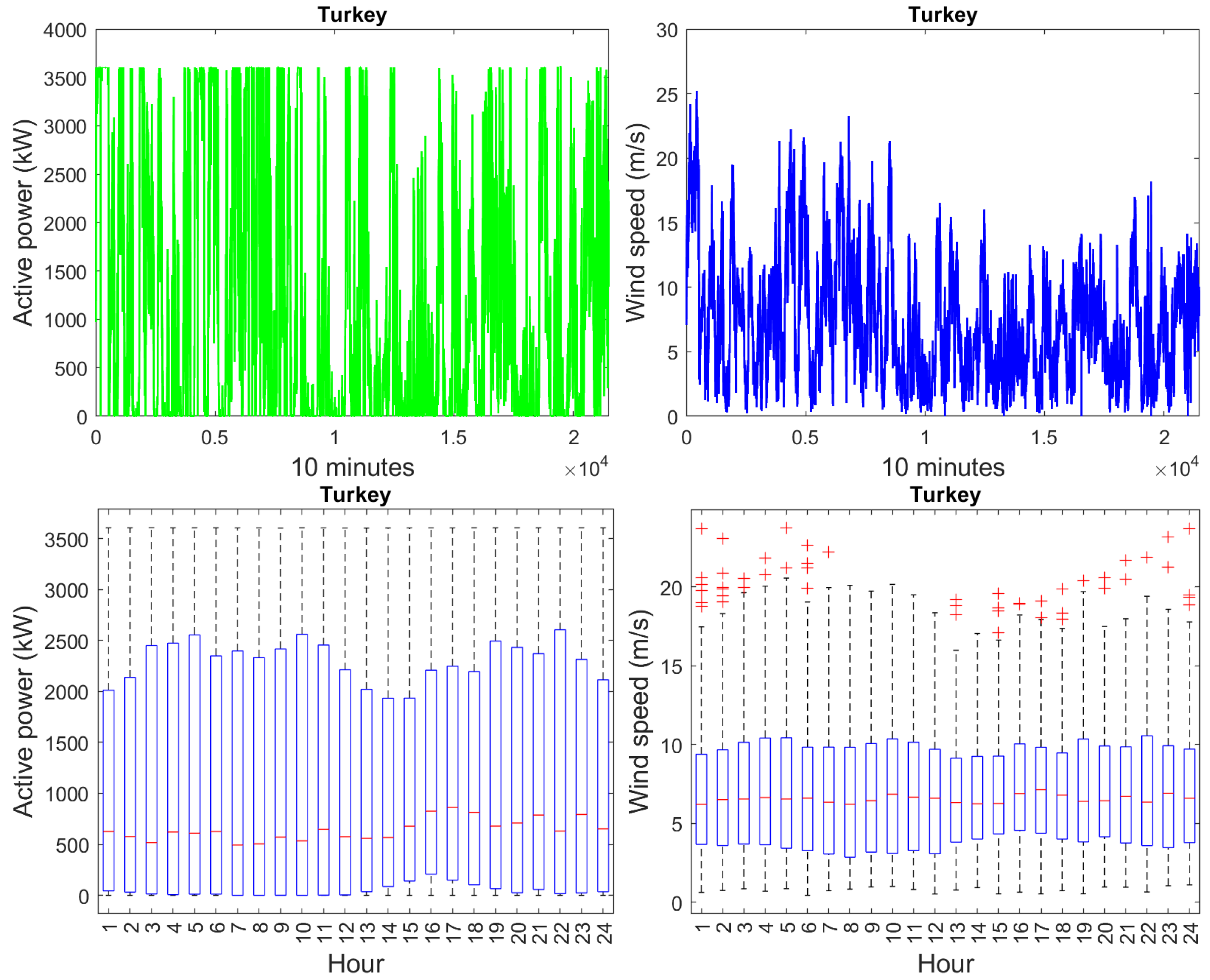
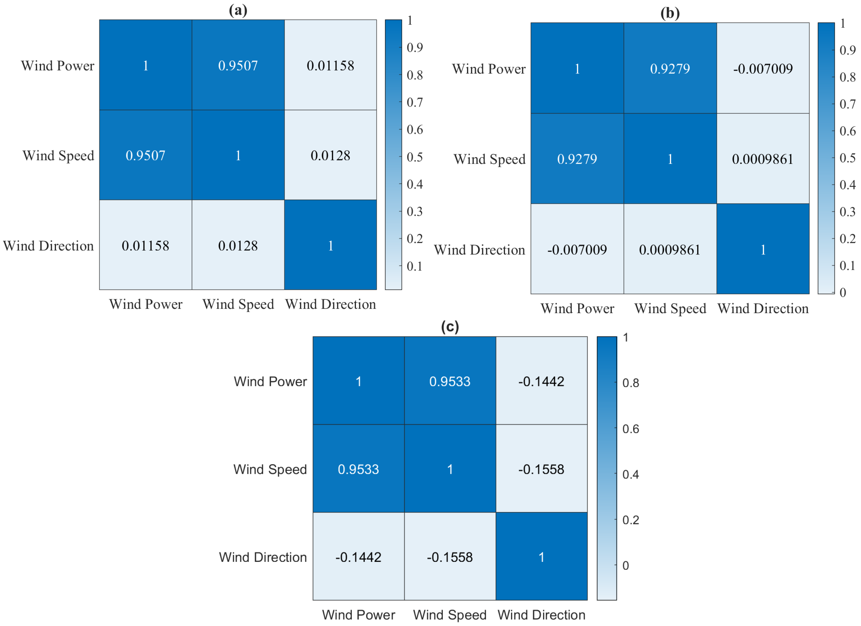
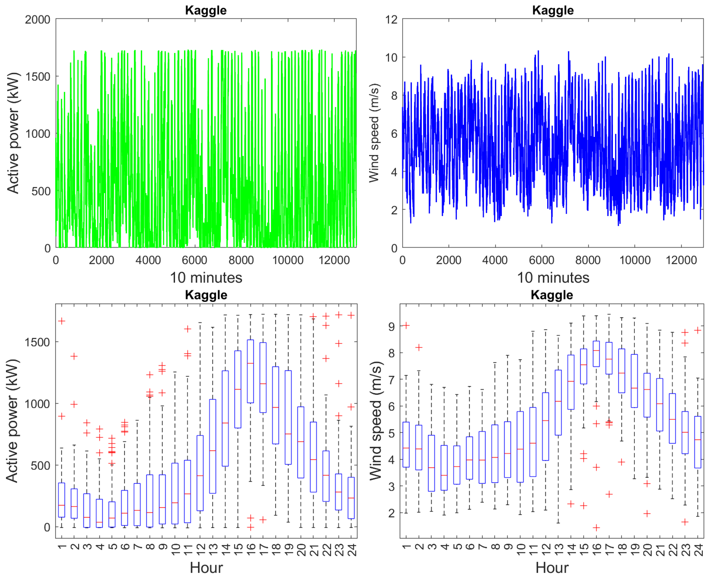
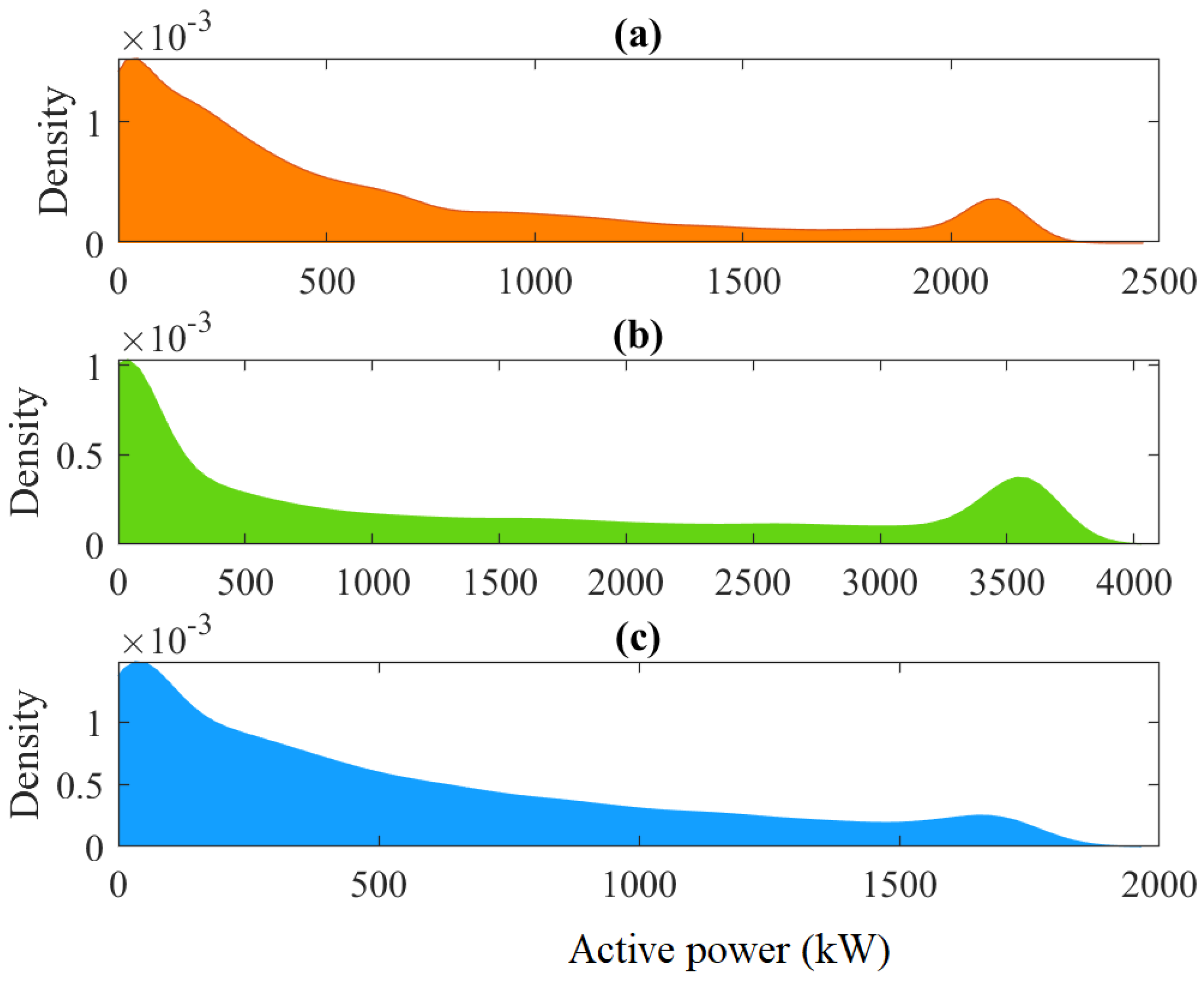
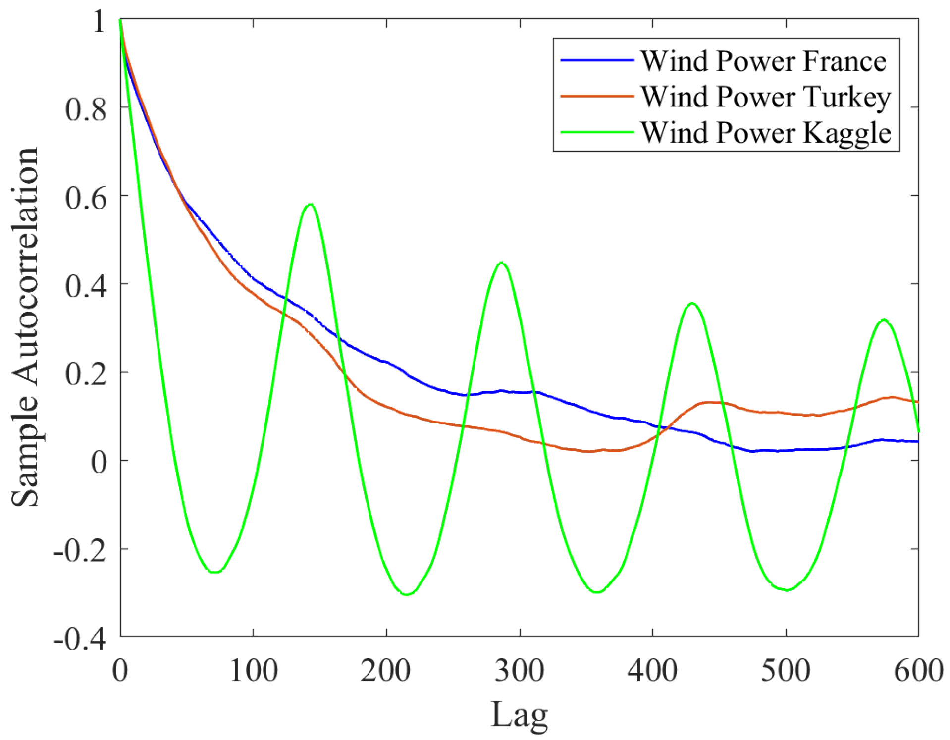
Three different datasets are used in this study to demonstrate the effectiveness of the considered machine learning models from France, Turkey, and Kaggle. Senvion MM82 wind turbines located in France recorded the first data in 2017 with a time resolution of ten minutes. The hub height of the Senvion MM82 wind turbine is 80 m. A wind turbine in Turkey gathers the second dataset that contains three variables (P, Ws, Wa) with ten minutes of time resolution. The last dataset from Kaggle was collected between January 2018 and March 2020 with time resolutions of 10 min. It contains twenty weather, turbine, and rotor features, namely active power, ambient temperature, bearing shaft temperature, blade 1 pitch angle, blade 2 pitch angle, blade 3 pitch angle, control box temperature, gearbox bearing temperature, gearbox oil temperature, generator rotations per minute (RPM), generator winding 1 temperature, generator winding 2 temperature, hub temperature, main box temperature, nacelle position, reactive power, rotor RPM, turbine status, wind direction, and wind speed. For France data, the investigated models are trained using data recorded from 1 February 2017 to 30 June 2017. For the Turkey data, the train data are collected from 1 February 2018 to 30 June 2018. Kaggle data contain some significant periods with missing values, which are discarded. We considered only periods with a few missing values. Specifically, we selected data for training from 1 January 2020 to 30 March 2020. We took the next three days of each training dataset for testing (i.e., 432 data points). A five-fold cross-validation procedure is adopted in training to avoid overfitting [90]. Figure 3, Figure 4 and Figure 5 show the wind power and wind speed time-series and the distribution of wind power and wind speed in the daytime from France, Turkey, and Kaggle wind turbines, respectively. This allows visual verification of the presence of data patterns and behavior over time. From Figure 3 and Figure 4, the presence of a long-term trend or seasonality in these data is not visually obvious. The bottom panel of Figure 5 (left and right) clearly shows the presence of a daily cycle in the hourly wind power and wind speed measurements, respectively.

Irregular variations without a daily cycle usually characterize the wind power time series, which is not the case with the studied Kaggle data. In the absence of additional information on the Kaggle wind power data (https://www.kaggle.com/theforcecoder/wind-power-forecasting) (accessed on 20 March 2022), it is not obvious to clarify the presence of this daily cycle (Figure 5).

3.1. Data Analysis

Figure 6 displays the probability density function (PDF) of the kernel density estimation fit to the wind power time-series data from three considered wind turbines. Visually from Figure 6, we can see that the wind power datasets are non-Gaussian distributed with positive support.

Figure 7 shows the autocorrelation function (ACF) plot of the wind power data collected from the three considered wind turbines. Generally speaking, the ACF graph is usually utilized to visually show the temporal correlations between $x_t$ and $x_{t+k}$, where $k=0,\cdots ,l$ and $x_t$ represents the wind power time series data [91]. Importantly, ACF measures the self-similarity of the wind power time-series data at different lag times [91]. Figure 7 indicates that the ACFs of France and Turkey wind power data from France tend slowly to zero, which indicates the presence of long-range dependence in this time-series data. Surprisingly, we observe that Kaggle wind power data are periodic with a period of 24 h. The length of the period is defined by the time difference between two successive peaks in the ACF plot. However, there is no obvious physical explanation of the source of this seasonality without more information from the Kaggle website. Usually, wind power output does not show period behaviors since it mainly depends on wind speed data, which are highly dynamic.

Figure 8 depicts the pairwise correlation coefficients between the wind speed, wind direction, and wind power from France, Turkey, and Kaggle wind turbines. We observe a very positive correlation between wind paper and wind speed and a weak correlation between wind power and wind direction. Overall, we conclude that the generated wind power is highly related to the input wind speed variation.

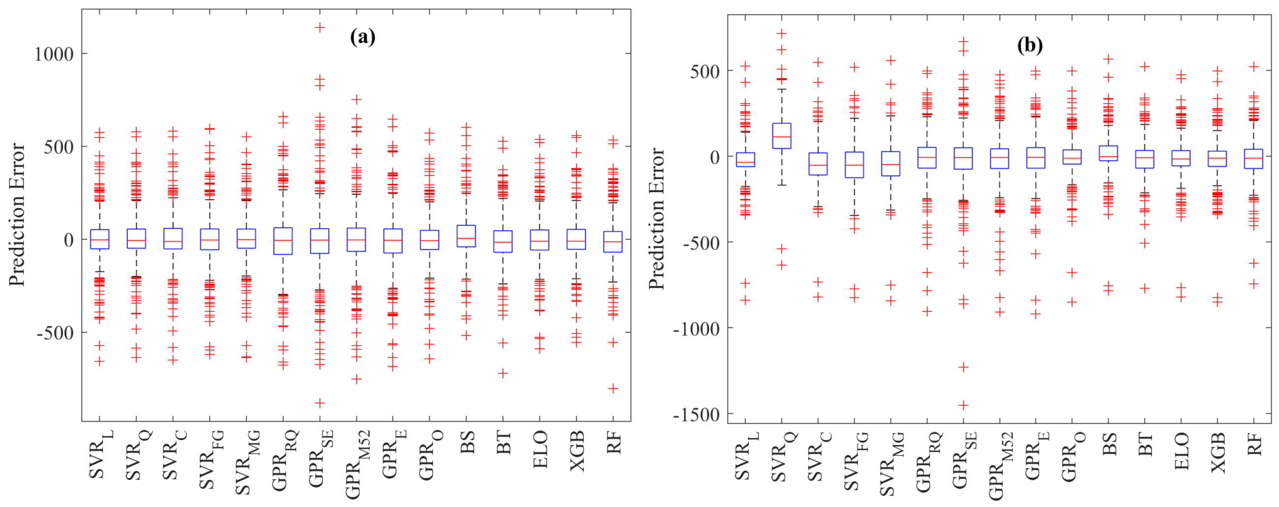
3.2. Forecasting Results

Three main experiments are conducted in this study to verify the performance of the seventeen considered machine learning models.

• Univariate forecasting using static models: In this scenario, we only used the past wind power time-series data to forecast the future trend of wind power. Each model is first trained using the wind power data and used to perform wind power forecasting.
• Univariate forecasting using dynamic models: In this experiment, the univariate forecasting of wind power is based on past and actual data. Considering information from lagged data is expected to obtain a better forecasting performance than the static models.
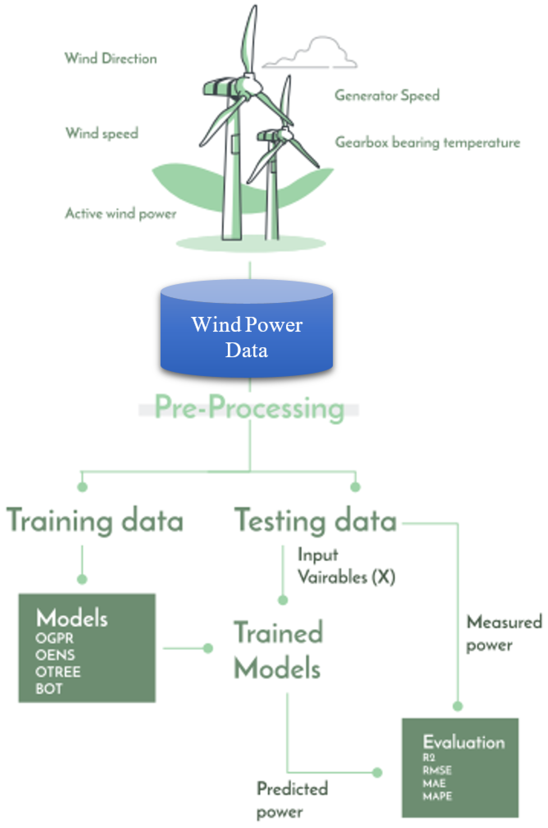
• Prediction of wind power: The prediction of wind power is conducted using other meteorological variables (e.g., wind speed and wind direction) as input. Specifically, we train each model to predict the next value of wind power based on input meteorological variables.

Wind Power Forecasting Using Static Models

In the first experiment, the considered machine learning models are trained using wind power training data for each wind turbine. We employed a five-fold cross-validation technique to train the investigated models. This study has been conducted using Matlab R2021b. Here, we used the BO method for the OGPR and OEL methods to obtain the optimal parameters minimizing the Mean Absolute Error between the predicted wind power and the actual wind power in the training stage.

Table 1. Hyperparameters search range and optimized hyperparameters via the BO algorithm.

Model	Hyperparameter Search Range	Optimized Hyperparameters
	-Sigma: 0.0001–1441.9316	-Sigma: 0.0080861
	-Basis function: Constant, Zero, Linear	-Basis function: Constant
GPRO	-Kernel function: Exp, M52, RQ, SE	-Kernel function: SE
	-Kernel scale: 0.498–2000	-Kernel scale: 1747.75
	-Standardize: true, false	-Standardize: True
	-Ensemble method: Bag, LSBoost	-Ensemble method: LSBoost
ELO	-Number of learners: 10–500	-Number of learners: 61
	-Learning rate: 0.001–1	-Learning rate: 0.20073
	-Minimum leaf size: 1–249	-Minimum leaf size: 3
	-Number of predictors to sample: 1–2	-Number of predictors to sample: 1

lists the computed values of the hyperparameters of considered models utilizing the BO algorithm. We omitted the results from the optimized SVR because it provides unsatisfactory results during the testing stage.

Here, the models forecast wind power without considering information from lagged data. We evaluate the performance of the trained models via test data recorded.

Table 2. Forecasting results using static models.

		France			Turkey			Kaggel
Models	RMSE (kW)	MAE (kW)	R2	RMSE (kW)	MAE (kW)	R2	RMSE (kW)	MAE (kW)	R2
SVR${}_L$	185.50	126.07	0.83	111.48	70.01	0.97	123.43	74.88	0.95
SVR${}_Q$	259.41	218.69	0.68	113.48	74.47	0.97	139.28	90.10	0.94
SVR${}_C$	187.64	124.63	0.83	120.46	88.44	0.96	123.49	79.41	0.95
SVR${}_{FG}$	186.16	123.82	0.83	131.25	98.08	0.95	124.30	80.81	0.95
SVR${}_{MG}$	186.32	123.68	0.83	133.22	101.86	0.95	124.32	80.10	0.95
GPR${}_{RQ}$	185.81	124.21	0.83	114.87	70.77	0.97	122.49	75.19	0.96
GPR${}_{SE}$	184.40	123.98	0.84	112.89	69.96	0.97	122.62	75.15	0.96
GPR${}_{M52}$	184.70	124.49	0.84	115.09	70.88	0.96	122.48	75.17	0.96
GPR${}_E$	183.23	124.42	0.84	122.63	78.13	0.96	121.62	75.47	0.96
GPR${}_O$	184.57	124.22	0.84	112.79	69.96	0.97	122.60	75.13	0.96
BS	183.66	124.33	0.84	114.34	71.78	0.97	129.71	82.38	0.95
BT	199.79	135.27	0.81	123.79	84.11	0.96	119.24	82.17	0.96
ELO	183.46	124.05	0.84	117.25	72.89	0.96	120.64	75.80	0.96
XGB	185.38	125.21	0.83	121.02	75.23	0.96	122.02	76.95	0.96
RF	223.40	148.95	0.76	185.13	115.01	0.91	132.52	91.95	0.95

lists the computed statistical scores (${\mathrm{R}}^2$, RMSE, MAE, and MAD) for each model based on the testing data for the three wind turbines (France, Turkey, and Kaggle). Three main observations can be extracted from the results in Table 2. The wind power data from the France turbine is very dynamic and complicated compared to the Turkey and Kaggle datasets. Except for the SVR${}_{CG}$ that provides poor forecasting results, the results in terms of ${\mathrm{R}}^2$ are within [0.75 0.83], [0.92 0.97], and [0.93 0.95] when using France, Turkey, and Kaggle datasets, respectively. The best result based on France data is obtained based on GPR${}_E$ with an ${\mathrm{R}}^2$ of 0.8384. In this experiment, the GPR${}_O$ reached the best results with an ${\mathrm{R}}^2$ of 0.9789 for the Turkey data, and the Bagging approach provided the best result for the Kaggle data with an ${\mathrm{R}}^2$ of 0.9578.

Next, we analyzed the distribution of the forecasting errors from the investigated models. Figure 9a–c shows the boxplots of the forecasting errors for each approach using test datasets from France, Turkey, and Kaggle data, respectively. The forecast error is the deviation between the measured and forecasted wind power measurements. The more compact the boxplot is, the more accurate the forecast is. Visually, we can see that the SVR${}_{CG}$ provides poor forecasting results with large boxplots. We can also see that the distributions of the forecasting errors of ensemble and kernel-based machine learning models are concentrated around zero, indicating satisfactory results, particularly for Turkey and Kaggle datasets.

As an illustration, the measured and forecasted wind power from the GPR model based on the three test datasets are given in Figure 10. The scatter plots show that the GPR model provides satisfactory forecasting results for Turkey and Kaggle datasets. The scatter plot of wind power from the France wind turbine indicates that the forecast does not closely follow the future trend of measured data.

3.3. Wind Power Prediction Using Dynamic Models

It is worth noticing from the first experiment that forecasting wind power time-series without considering the past information has not led to good forecasting results. In addition, wind power data exhibit a dynamic nature, as shown in ACF plots (Figure 7). This experiment aims to investigate the accuracy of the machine learning methods when including information from past data. To this end, dynamic characteristics of wind power data can be considered using lagged data to construct the prediction models. We used time-lagged wind power data as input to predict wind power. After evaluating the length of the input sequence on the forecasting output, the length of time-lagged data adopted is 5. This means that we use the previous five data points to predict the next wind power observation.

Table 3. Hyperparameters search range and optimized hyperparameters using the BO algorithm.

Model	Hyperparameter Search Range	Optimized Hyperparameters
	-Sigma: 0.0001–1441.9316	-Sigma: 0.049216
	-Basis function: Constant, Zero, Linear	-Basis function: Linear
GPRO	-Kernel function: Exp, M52, RQ, SE	-Kernel function: RQ
	-Kernel scale: 0.498–2000	-Kernel scale: 1145.0171
	-Standardize: true, false	-Standardize: True
	-Ensemble method: Bag, LSBoost	-Ensemble method: Bag
ELO	-Number of learners: 10–500	-Number of learners: 19
	-Learning rate: 0.001–1	-Learning rate: 0.2
	-Minimum leaf size: 1–249	-Minimum leaf size: 34
	-Number of predictors to sample: 1–5	-Number of predictors to sample: 4

summarizes the obtained values of the hyperparameters of considered dynamic models via the BO algorithm.

Table 4. Forecasting results using dynamic models.

		France			Turkey			Kaggel
Models	RMSE (kW)	MAE (kW)	R2	RMSE (kW)	MAE (kW)	R2	RMSE (kW)	MAE (kW)	R2
SVR${}_L$	130.89	85.36	0.91	111.98	73.04	0.97	130.89	85.36	0.91
SVR${}_Q$	130.77	85.06	0.91	171.45	133.97	0.92	130.77	85.06	0.91
SVR${}_C$	131.71	86.98	0.91	122.53	90.98	0.96	131.71	86.98	0.91
SVR${}_{FG}$	149.47	97.84	0.89	133.39	100.31	0.95	149.47	97.84	0.89
SVR${}_{MG}$	132.07	85.76	0.91	124.17	91.53	0.96	132.07	85.76	0.91
GPR${}_{RQ}$	165.33	112.81	0.86	143.97	93.44	0.94	165.33	112.81	0.86
GPR${}_{SE}$	199.63	125.11	0.80	176.64	101.93	0.92	199.63	125.11	0.80
GPR${}_{M52}$	170.63	110.82	0.85	148.86	94.90	0.94	170.63	110.82	0.85
GPR${}_E$	160.65	108.14	0.87	133.34	85.20	0.95	160.65	108.14	0.87
GPR${}_O$	129.06	84.94	0.92	109.62	68.87	0.97	129.06	84.94	0.92
BS	129.26	87.08	0.92	114.71	71.94	0.96	129.26	87.08	0.92
BT	129.62	88.27	0.91	112.21	75.21	0.97	129.62	88.27	0.91
ELO	127.37	86.15	0.92	114.86	72.74	0.96	127.37	86.15	0.92
XGB	129.68	88.16	0.91	117.28	73.17	0.96	129.68	88.16	0.91
RF	133.70	90.41	0.91	118.87	80.09	0.96	133.70	90.41	0.91

lists the evaluation metrics (RMSE, MAE, and R${}^2$) obtained using the fifteen considered models with time-lagged data based on testing data from the three studied wind turbines. Table 4 indicates that the dynamic models improved wind power prediction, particularly for France data. Similar conclusions still arise when comparing the performance of the considered models. Importantly, GPRO and ensemble models achieved superior forecast performance than the other investigated models.

Figure 11 depicts the boxplots of the forecast errors from the investigated models based on testing data from the three turbines (France, Turkey, and France). It can be seen that ensemble models and GPRO provide less forecasting errors than other models. There is no single approach dominating the others for all cases, but on average, the GPRO and ensemble learning models achieved satisfactory results.

As a visual illustration, Figure 12 displays the scatter graphs and plots of the measured testing data together with the ELO model forecasts of wind power. To simplify visual readability, the results from the other models are omitted. Figure 12 indicates that the forecasted values of wind power from the ELO models are closer to the actual data collected from France, Turkey, and Kaggle, indicating good forecast performance.

Figure 13 provides a visual comparison between the average R${}^2$ values obtained from static models and dynamic models. We observe that the use of dynamic models leads to improved prediction results of wind power compared to statistical models, particularly for ensemble models (i.e., Boosting, bagging, XGBoost, and RF) and the GPRO model. This experiment revealed that incorporating information from past data in building prediction models significantly improves the prediction accuracy of machine learning models.

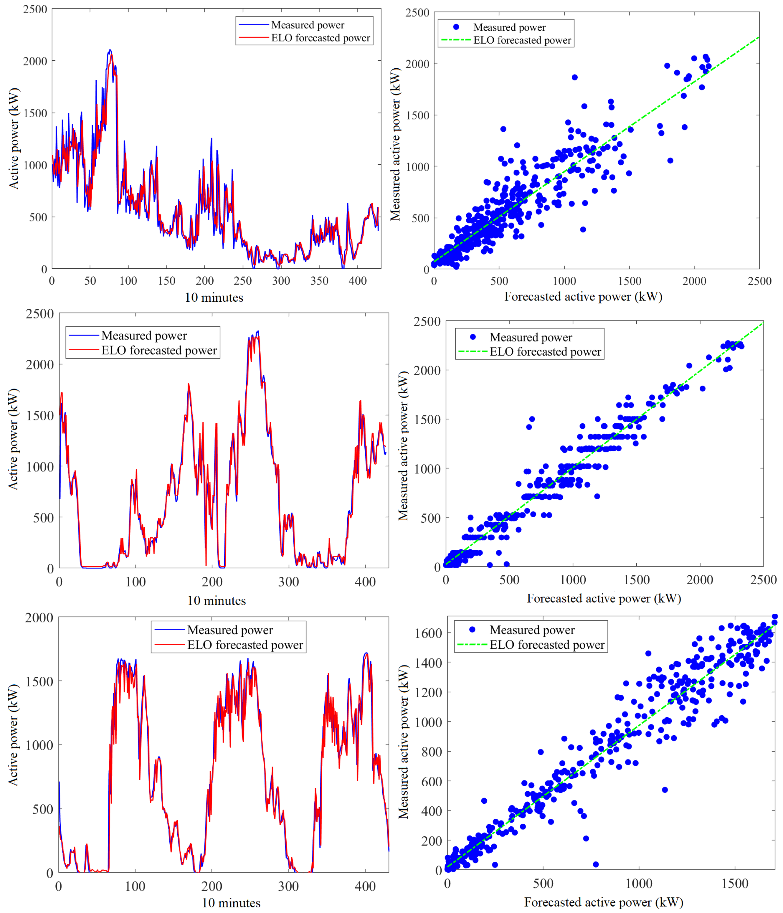
3.4. Wind Power Prediction

The previous experiment showed that using information from past data in building prediction models improved the prediction accuracy of wind power. This last experiment investigates the capacity of considered machine learning models for wind power prediction using meteorological variables as input variables (i.e., wind direction and wind speed). As the wind speed is highly correlated with the produced wind power (Figure 8), it is expected that employing information from the wind direction and wind speed will improve the prediction accuracy of wind power. To this end, the fifteen models are trained using training data to predict wind power using wind direction and wind speed as input variables (covariate information). After that, each model is used to predict wind power for the testing data.

Table 5. Prediction results of the fifteen models using France data.

Models	RMSE (kW)	MAE (kW)	R2
SVR${}_L$	129.91	102.80	0.91
SVR${}_Q$	85.22	59.08	0.96
SVR${}_C$	88.57	62.93	0.96
SVR${}_{FG}$	87.52	59.26	0.96
SVR${}_{MG}$	83.44	57.12	0.96
GPR${}_{RQ}$	76.91	48.89	0.97
GPR${}_{SE}$	78.54	50.03	0.97
GPR${}_{M52}$	76.54	48.26	0.97
GPR${}_E$	76.91	46.94	0.97
GPR${}_O$	69.47	41.13	0.98
BS	73.77	47.54	0.97
BT	42.28	21.41	0.99
ELO	84.95	52.87	0.96
XGB	78.32	46.09	0.97
RF	56.74	37.07	0.98

reports the prediction results in terms of RMSE, MAE, and R${}^2$ obtained using the fifteen machine learning models based on test data from the France wind turbine. The results in Table 5 show the satisfactory performance of kernel-based learning methods and ensemble learning methods in predicting wind power with high accuracy, with R${}^2$ values around 0.96, except for linear SVR (R${}^2$ = 0.91). This could be explained by the limitation of the linear SVR model in capturing process nonlinearity in wind power data. The bagging trees model dominated all the other models by capturing almost 99% of the variance in wind power data (i.e., R${}^2$ = 0.99). It is followed by RF and GPR (R${}^2$ = 0.98%).

Figure 14 illustrates the boxplots of the prediction errors for each approach using test datasets. From Figure 14, we observe that the boxplot related to the BT and GPRO and ensemble models are concentrated around zero, indicating the better prediction performance of these models. Visually, we can see also that ensemble models (BT, BS, RF, and XGBoost) and GPRO with narrower boxes and whiskers reach superior performance compared to the other models.

The measured and predicted wind power data from the ensemble models are displayed in Figure 15. Visual inspection of time series plots in Figure 15 shows that the predicted wind power from the investigated models closely followed the measured wind power data.

As expected, the prediction accuracy of all considered models increased after using information from input variables (wind speed and wind direction). The use of information from input variables increased the wind power prediction significantly. Specifically, the RMSE value of the BT model has been decreased by 157.51, and the ${\mathrm{R}}^2$ value increased by 0.18 compared to the BT with input variables. The last finding is because the incorporated meteorological variables, particularly wind speed, have great impact on generating wind power. Thus, when information from meteorological variables is available, its consideration in the machine learning models will allow for more accurate wind power prediction.

From Table 5, it can be observed that ensemble learning-driven models provided promising wind power prediction. Theoretically, it is clear that the variance of prediction employing n learners could be decreased to $1/n$ of the variance of a single learner. Thus, the use of a large number of learners is advantageous because it generally results in reduced variance compared to standalone learners of a small set of learners. For instance, to understand how the bagging approach reduces the prediction error, let us consider the following regression problem with base regressors $b_1\left(x\right),\cdots ,b_n\left(x\right)$. Assume that an ideal target function of true answers $y\left(x\right)$ obtained from a given set of inputs is known. Furthermore, assume that the distribution $p\left(x\right)$ is specified. Then, the error is obtained for each regression function as follows [58]:

$${\epsilon }_i\left(x\right)=b_i\left(x\right)-y\left(x\right),i=1,\cdots ,n$$

(13)

The mean square prediction error is formulated as [58]:

$$E_x\left[{\left(b_i\left(x\right)-y\left(x\right)\right)}^2\right]=E_x\left[{\epsilon }_i^2\left(x\right)\right].$$

(14)

Then, the mean prediction error over all the regression functions is expressed as [58]

$$E_1=\frac{1}{n}{E}_x\left[{\epsilon }_i^2\left(x\right)\right]$$

(15)

Assume that the errors are unbiased and uncorrelated, then we can write [58]:

$$\begin{array}{ccc}\hfill E_x\left[{\epsilon }_i\left(x\right)\right]& =& 0,\hfill \\ \hfill E_x\left[{\epsilon }_i\left(x\right){\epsilon }_j\left(x\right)\right]& =& 0,i\ne j.\hfill \end{array}$$

(16)

The regression function can be computed as [58]:

$$a\left(x\right)=\frac{1}{n}\sum _{i=1}^n{b}_i\left(x\right).$$

(17)

Thus, its mean square error is provided by [58]

$$\begin{array}{ccc}\hfill E_n& =& E_x{\left[\frac{1}{n}\sum _{i=1}^n{b}_i\left(x\right)-y\left(x\right)\right]}^2\hfill \\ \hfill & =& E_x{\left[\frac{1}{n}\sum _{i=1}^n{\epsilon }_i\right]}^2\hfill \\ \hfill & =& \frac{1}{n^2}{E}_x\left[\sum _{i=1}^n{\epsilon }_i^2\left(x\right)+\sum _{i\ne j}{\epsilon }_i\left(x\right){\epsilon }_j\left(x\right)\right]\hfill \\ \hfill & =& \frac{1}{n}{E}_1.\hfill \end{array}$$

(18)

The central characteristic of ensemble learning-driven models is their capability to reduce forecasting error.

Overall, this study investigated and compared the performance of both static and dynamic machine learning models for predicting wind power. Essentially, the results indicated that the dynamic models that incorporate past data information provide superior prediction performance compared to the static models. In addition, the prediction accuracy is significantly improved when considering methodological variables (i.e., wind speed and wind direction). The optimized dynamic GPR model provided a comparable prediction performance as ensemble learning models in predicting wind power.

4. Conclusions

Accurate forecasting of wind power is essential for quantifying and managing the energy budget in the power grid. This study first applied and compared several machine learning approaches to model the nonlinear wind power dynamics and forecast the future trends of wind power. Specifically, kernel-driven machine learning models (SVR and GPR) and ensemble learning models (Boosting, Bagging, XGBoost, and RF) are considered in this comparative study. Wind power data from three wind turbines are used to assess the effectiveness of the machine learning models in this study. The results revealed that using dynamic models that consider relevant information from past observations of wind power series improved the prediction results compared to static models. Furthermore, this study showed that including information from input variables (i.e., wind speed and wind direction) further improves the prediction results. We observe that there is no single approach dominating the others for all experiments, but on average, the GPR models and ensemble models reached a satisfactory prediction performance, with an R² of about 0.95.

Despite the satisfactory wind power prediction results using the dynamic machine learning techniques, future works will be aimed at improving the robustness of the machine learning techniques to noisy wind power measurements by developing wavelet-based dynamic machine learning methods. Another direction of improvement is to incorporate explanatory variables, such as meteorological measurements, in constructing the machine learning techniques to further improve prediction quality. Furthermore, an interesting future work is to develop machine-learning-driven fault detection methods for wind turbines monitoring. More specifically, the dynamic machine learning models presented in this study can be used to model the normal operating condition of the inspected wind turbines, and statistical monitoring charts, such as exponentially weighted moving average and generalized likelihood tests, can be applied for fault detection [92].

References

1. American Wind Energy Association (AWEA). Wind Powers America First Quarter 2020 Report; American Wind Energy Association (AWEA): Washington, DC, USA, 2020. [Google Scholar]
2. Hanifi, S.; Liu, X.; Lin, Z.; Lotfian, S. A critical review of wind power forecasting methods—past, present and future. Energies 2020, 13, 3764. [Google Scholar] [CrossRef]
3. Treiber, N.A.; Heinermann, J.; Kramer, O. Wind power prediction with machine learning. In Computational Sustainability; Springer: Berlin/Heidelberg, Germany, 2016; pp. 13–29. [Google Scholar]
4. Yang, M.; Wang, S. A review of wind power forecasting & prediction. In Proceedings of the 2016 International Conference on Probabilistic Methods Applied to Power Systems (PMAPS), Beijing, China, 16–20 October 2016; pp. 1–7. [Google Scholar]
5. Ouyang, T.; Zha, X.; Qin, L.; He, Y.; Tang, Z. Prediction of wind power ramp events based on residual correction. Renew. Energy 2019, 136, 781–792. [Google Scholar] [CrossRef]
6. Ding, F.; Tian, Z.; Zhao, F.; Xu, H. An integrated approach for wind turbine gearbox fatigue life prediction considering instantaneously varying load conditions. Renew. Energy 2018, 129, 260–270. [Google Scholar] [CrossRef]
7. Han, S.; Qiao, Y.H.; Yan, J.; Liu, Y.Q.; Li, L.; Wang, Z. Mid-to-long term wind and photovoltaic power generation prediction based on copula function and long short term memory network. Appl. Energy 2019, 239, 181–191. [Google Scholar] [CrossRef]
8. Tascikaraoglu, A.; Uzunoglu, M. A review of combined approaches for prediction of short-term wind speed and power. Renew. Sustain. Energy Rev. 2014, 34, 243–254. [Google Scholar] [CrossRef]
9. Bouyeddou, B.; Harrou, F.; Saidi, A.; Sun, Y. An Effective Wind Power Prediction using Latent Regression Models. In Proceedings of the 2021 International Conference on ICT for Smart Society (ICISS), Bandung, Indonesia, 2–4 August 2021; pp. 1–6. [Google Scholar]
10. Yan, J.; Ouyang, T. Advanced wind power prediction based on data-driven error correction. Energy Convers. Manag. 2019, 180, 302–311. [Google Scholar] [CrossRef]
11. Karakuş, O.; Kuruoğlu, E.E.; Altınkaya, M.A. One-day ahead wind speed/power prediction based on polynomial autoregressive model. IET Renew. Power Gener. 2017, 11, 1430–1439. [Google Scholar] [CrossRef] [Green Version]
12. Eissa, M.; Yu, J.; Wang, S.; Liu, P. Assessment of wind power prediction using hybrid method and comparison with different models. J. Electr. Eng. Technol. 2018, 13, 1089–1098. [Google Scholar]
13. Rajagopalan, S.; Santoso, S. Wind power forecasting and error analysis using the autoregressive moving average modeling. In Proceedings of the 2009 IEEE Power & Energy Society General Meeting, Calgary, AB, Canada, 26–30 July 2009; pp. 1–6. [Google Scholar]
14. Singh, P.K.; Singh, N.; Negi, R. Wind Power Forecasting Using Hybrid ARIMA-ANN Technique. In Ambient Communications and Computer Systems; Springer: Berlin/Heidelberg, Germany, 2019; pp. 209–220. [Google Scholar]
15. Bhaskar, K.; Singh, S. AWNN-assisted wind power forecasting using feed-forward neural network. IEEE Trans. Sustain. Energy 2012, 3, 306–315. [Google Scholar] [CrossRef]
16. Chen, N.; Qian, Z.; Nabney, I.T.; Meng, X. Wind power forecasts using Gaussian processes and numerical weather prediction. IEEE Trans. Power Syst. 2013, 29, 656–665. [Google Scholar] [CrossRef] [Green Version]
17. Azimi, R.; Ghofrani, M.; Ghayekhloo, M. A hybrid wind power forecasting model based on data mining and wavelets analysis. Energy Convers. Manag. 2016, 127, 208–225. [Google Scholar] [CrossRef]
18. Yang, L.; He, M.; Zhang, J.; Vittal, V. Support-vector-machine-enhanced markov model for short-term wind power forecast. IEEE Trans. Sustain. Energy 2015, 6, 791–799. [Google Scholar] [CrossRef]
19. Ti, Z.; Deng, X.W.; Zhang, M. Artificial Neural Networks based wake model for power prediction of wind farm. Renew. Energy 2021, 172, 618–631. [Google Scholar] [CrossRef]
20. Saroha, S.; Aggarwal, S. Wind power forecasting using wavelet transforms and neural networks with tapped delay. CSEE J. Power Energy Syst. 2018, 4, 197–209. [Google Scholar] [CrossRef]
21. Dowell, J.; Pinson, P. Very-short-term probabilistic wind power forecasts by sparse vector autoregression. IEEE Trans. Smart Grid 2015, 7, 763–770. [Google Scholar] [CrossRef] [Green Version]
22. Wu, J.; Ji, T.; Li, M.; Wu, P.; Wu, Q. Multistep wind power forecast using mean trend detector and mathematical morphology-based local predictor. IEEE Trans. Sustain. Energy 2015, 6, 1216–1223. [Google Scholar] [CrossRef]
23. Demolli, H.; Dokuz, A.S.; Ecemis, A.; Gokcek, M. Wind power forecasting based on daily wind speed data using machine learning algorithms. Energy Convers. Manag. 2019, 198, 111823. [Google Scholar] [CrossRef]
24. Lekkas, D.; Price, G.D.; Jacobson, N.C. Using smartphone app use and lagged-ensemble machine learning for the prediction of work fatigue and boredom. Comput. Hum. Behav. 2022, 127, 107029. [Google Scholar] [CrossRef]
25. Bi, J.W.; Han, T.Y.; Li, H. International tourism demand forecasting with machine learning models: The power of the number of lagged inputs. Tour. Econ. 2020, 1354816620976954. [Google Scholar] [CrossRef]
26. Shang, H.L. Dynamic principal component regression for forecasting functional time series in a group structure. Scand. Actuar. J. 2020, 2020, 307–322. [Google Scholar] [CrossRef]
27. Liu, Y.; Sun, Y.; Infield, D.; Zhao, Y.; Han, S.; Yan, J. A hybrid forecasting method for wind power ramp based on orthogonal test and support vector machine (OT-SVM). IEEE Trans. Sustain. Energy 2016, 8, 451–457. [Google Scholar] [CrossRef] [Green Version]
28. Yuan, X.; Chen, C.; Yuan, Y.; Huang, Y.; Tan, Q. Short-term wind power prediction based on LSSVM–GSA model. Energy Convers. Manag. 2015, 101, 393–401. [Google Scholar] [CrossRef]
29. Buturache, A.N.; Stancu, S. Wind Energy Prediction Using Machine Learning. Low Carbon Econ. 2021, 12, 1. [Google Scholar] [CrossRef]
30. Liu, T.; Wei, H.; Zhang, K. Wind power prediction with missing data using Gaussian process regression and multiple imputation. Appl. Soft Comput. 2018, 71, 905–916. [Google Scholar] [CrossRef]
31. Deng, Y.; Jia, H.; Li, P.; Tong, X.; Qiu, X.; Li, F. A deep learning methodology based on bidirectional gated recurrent unit for wind power prediction. In Proceedings of the 2019 14th IEEE Conference on Industrial Electronics and Applications (ICIEA), Xi’an, China, 19–21 June 2019; pp. 591–595. [Google Scholar]
32. Xiaoyun, Q.; Xiaoning, K.; Chao, Z.; Shuai, J.; Xiuda, M. Short-term prediction of wind power based on deep long short-term memory. In Proceedings of the 2016 IEEE PES Asia-Pacific Power and Energy Engineering Conference (APPEEC), Xi’an, China, 25–28 October 2016; pp. 1148–1152. [Google Scholar]
33. Bibi, N.; Shah, I.; Alsubie, A.; Ali, S.; Lone, S.A. Electricity Spot Prices Forecasting Based on Ensemble Learning. IEEE Access 2021, 9, 150984–150992. [Google Scholar] [CrossRef]
34. Shah, I.; Iftikhar, H.; Ali, S.; Wang, D. Short-term electricity demand forecasting using components estimation technique. Energies 2019, 12, 2532. [Google Scholar] [CrossRef] [Green Version]
35. Lisi, F.; Shah, I. Forecasting next-day electricity demand and prices based on functional models. Energy Syst. 2020, 11, 947–979. [Google Scholar] [CrossRef]
36. Su, M.; Zhang, Z.; Zhu, Y.; Zha, D.; Wen, W. Data driven natural gas spot price prediction models using machine learning methods. Energies 2019, 12, 1680. [Google Scholar] [CrossRef] [Green Version]
37. Ghoddusi, H.; Creamer, G.G.; Rafizadeh, N. Machine learning in energy economics and finance: A review. Energy Econ. 2019, 81, 709–727. [Google Scholar] [CrossRef]
38. Toubeau, J.F.; Pardoen, L.; Hubert, L.; Marenne, N.; Sprooten, J.; De Grève, Z.; Vallée, F. Machine learning-assisted outage planning for maintenance activities in power systems with renewables. Energy 2022, 238, 121993. [Google Scholar] [CrossRef]
39. Cai, C.; Kamada, Y.; Maeda, T.; Hiromori, Y.; Zhou, S.; Xu, J. Prediction of power generation of two 30 kW Horizontal Axis Wind Turbines with Gaussian model. Energy 2021, 231, 121075. [Google Scholar]
40. Cheng, B.; Du, J.; Yao, Y. Machine learning methods to assist structure design and optimization of Dual Darrieus Wind Turbines. Energy 2021, 244, 122643. [Google Scholar] [CrossRef]
41. Reddy, S.R. A machine learning approach for modeling irregular regions with multiple owners in wind farm layout design. Energy 2021, 220, 119691. [Google Scholar] [CrossRef]
42. Xie, Y.; Zhao, K.; Sun, Y.; Chen, D. Gaussian processes for short-term traffic volume forecasting. Transp. Res. Rec. 2010, 2165, 69–78. [Google Scholar] [CrossRef] [Green Version]
43. Harrou, F.; Saidi, A.; Sun, Y.; Khadraoui, S. Monitoring of photovoltaic systems using improved kernel-based learning schemes. IEEE J. Photovolt. 2021, 11, 806–818. [Google Scholar] [CrossRef]
44. Lee, J.; Wang, W.; Harrou, F.; Sun, Y. Wind power prediction using ensemble learning-based models. IEEE Access 2020, 8, 61517–61527. [Google Scholar] [CrossRef]
45. Williams, C.K.; Rasmussen, C.E. Gaussian Processes for Regression. 1996. Available online: https://is.mpg.de/publications/2468 (accessed on 10 February 2022).
46. MacKay, D.J. Gaussian Processes-A Replacement for Supervised Neural Networks? 1997. Available online: http://www.inference.org.uk/mackay/gp.pdf (accessed on 10 February 2022).
47. Yang, W.; Deng, M.; Xu, F.; Wang, H. Prediction of hourly PM2. 5 using a space-time support vector regression model. Atmos. Environ. 2018, 181, 12–19. [Google Scholar] [CrossRef]
48. Schulz, E.; Speekenbrink, M.; Krause, A. A tutorial on Gaussian process regression: Modelling, exploring, and exploiting functions. J. Math. Psychol. 2018, 85, 1–16. [Google Scholar] [CrossRef]
49. Seeger, M. Gaussian processes for machine learning. Int. J. Neural Syst. 2004, 14, 69–106. [Google Scholar] [CrossRef] [Green Version]
50. Nguyen, V.H.; Le, T.T.; Truong, H.S.; Le, M.V.; Ngo, V.L.; Nguyen, A.T.; Nguyen, H.Q. Applying Bayesian Optimization for Machine Learning Models in Predicting the Surface Roughness in Single-Point Diamond Turning Polycarbonate. Math. Probl. Eng. 2021, 2021, 6815802. [Google Scholar] [CrossRef]
51. García-Nieto, P.J.; García-Gonzalo, E.; Puig-Bargués, J.; Duran-Ros, M.; de Cartagena, F.R.; Arbat, G. Prediction of outlet dissolved oxygen in micro-irrigation sand media filters using a Gaussian process regression. Biosyst. Eng. 2020, 195, 198–207. [Google Scholar] [CrossRef]
52. Murphy, K.P. Machine Learning: A Probabilistic Perspective; MIT Press: Cambridge, MA, USA, 2012. [Google Scholar]
53. Yu, P.S.; Chen, S.T.; Chang, I.F. Support vector regression for real-time flood stage forecasting. J. Hydrol. 2006, 328, 704–716. [Google Scholar] [CrossRef]
54. Hong, W.C.; Dong, Y.; Chen, L.Y.; Wei, S.Y. SVR with hybrid chaotic genetic algorithms for tourism demand forecasting. Appl. Soft Comput. 2011, 11, 1881–1890. [Google Scholar] [CrossRef]
55. Smola, A.J.; Schölkopf, B. A tutorial on support vector regression. Stat. Comput. 2004, 14, 199–222. [Google Scholar] [CrossRef] [Green Version]
56. Zeroual, A.; Harrou, F.; Sun, Y. Predicting road traffic density using a machine learning-driven approach. In Proceedings of the 2021 International Conference on Electrical, Computer and Energy Technologies (ICECET), Cape Town, South Africa, 9–10 December 2021; pp. 1–6. [Google Scholar]
57. Khaldi, B.; Harrou, F.; Benslimane, S.M.; Sun, Y. A Data-Driven Soft Sensor for Swarm Motion Speed Prediction using Ensemble Learning Methods. IEEE Sens. J. 2021, 21, 19025–19037. [Google Scholar] [CrossRef]
58. Lee, J.; Wang, W.; Harrou, F.; Sun, Y. Reliable solar irradiance prediction using ensemble learning-based models: A comparative study. Energy Convers. Manag. 2020, 208, 112582. [Google Scholar] [CrossRef] [Green Version]
59. Kari, T.; Gao, W.; Tuluhong, A.; Yaermaimaiti, Y.; Zhang, Z. Mixed kernel function support vector regression with genetic algorithm for forecasting dissolved gas content in power transformers. Energies 2018, 11, 2437. [Google Scholar] [CrossRef] [Green Version]
60. Protopapadakis, E.; Voulodimos, A.; Doulamis, N. An investigation on multi-objective optimization of feedforward neural network topology. In Proceedings of the 2017 8th International Conference on Information, Intelligence, Systems & Applications (IISA), Larnaca, Cyprus, 27–30 August 2017; pp. 1–6. [Google Scholar]
61. Shahriari, B.; Swersky, K.; Wang, Z.; Adams, R.P.; De Freitas, N. Taking the human out of the loop: A review of Bayesian optimization. Proc. IEEE 2015, 104, 148–175. [Google Scholar] [CrossRef] [Green Version]
62. Snoek, J.; Larochelle, H.; Adams, R.P. Practical bayesian optimization of machine learning algorithms. Adv. Neural Inf. Process. Syst. 2012, 25, 1–9. [Google Scholar]
63. Alali, Y.; Harrou, F.; Sun, Y. A proficient approach to forecast COVID-19 spread via optimized dynamic machine learning models. Sci. Rep. 2022, 12, 2467. [Google Scholar] [CrossRef]
64. Springenberg, J.T.; Klein, A.; Falkner, S.; Hutter, F. Bayesian optimization with robust Bayesian neural networks. Adv. Neural Inf. Process. Syst. 2016, 29, 4134–4142. [Google Scholar]
65. Freund, Y.; Schapire, R.E. A decision-theoretic generalization of on-line learning and an application to boosting. J. Comput. Syst. Sci. 1997, 55, 119–139. [Google Scholar] [CrossRef] [Green Version]
66. Schapire, R.E.; Freund, Y.; Bartlett, P.; Lee, W.S. Boosting the margin: A new explanation for the effectiveness of voting methods. Ann. Stat. 1998, 26, 1651–1686. [Google Scholar]
67. Schapire, R.E. The boosting approach to machine learning: An overview. In Nonlinear Estimation and Classification; Springer: Berlin/Heidelberg, Germany, 2003; pp. 149–171. [Google Scholar]
68. Bühlmann, P.; Hothorn, T. Boosting algorithms: Regularization, prediction and model fitting. Stat. Sci. 2007, 22, 477–505. [Google Scholar]
69. Chen, T.; Guestrin, C. Xgboost: A scalable tree boosting system. In Proceedings of the 22nd ACM Sigkdd International Conference on Knowledge Discovery and Data Mining, San Francisco, CA, USA, 13–17 August 2016; pp. 785–794. [Google Scholar]
70. Breiman, L. Arcing classifiers. Ann. Stat. 1996, 26, 123–140. [Google Scholar]
71. Breiman, L. Prediction games and arcing algorithms. Neural Comput. 1999, 11, 1493–1517. [Google Scholar] [CrossRef]
72. Friedman, J.; Hastie, T.; Tibshirani, R. Additive logistic regression: A statistical view of boosting (with discussion and a rejoinder by the authors). Ann. Stat. 2000, 28, 337–407. [Google Scholar] [CrossRef]
73. Friedman, J.H. Greedy function approximation: A gradient boosting machine. Ann. Stat. 2001, 29, 1189–1232. [Google Scholar] [CrossRef]
74. Breiman, L. Bagging predictors. Mach. Learn. 1996, 24, 123–140. [Google Scholar] [CrossRef] [Green Version]
75. Zhang, Y.; Haghani, A. A gradient boosting method to improve travel time prediction. Transp. Res. Part C Emerg. Technol. 2015, 58, 308–324. [Google Scholar] [CrossRef]
76. Harrou, F.; Saidi, A.; Sun, Y. Wind power prediction using bootstrap aggregating trees approach to enabling sustainable wind power integration in a smart grid. Energy Convers. Manag. 2019, 201, 112077. [Google Scholar] [CrossRef]
77. Ruiz-Abellón, M.D.C.; Gabaldón, A.; Guillamón, A. Load forecasting for a campus university using ensemble methods based on regression trees. Energies 2018, 11, 2038. [Google Scholar] [CrossRef] [Green Version]
78. Bauer, E.; Kohavi, R. An empirical comparison of voting classification algorithms: Bagging, boosting, and variants. Mach. Learn. 1999, 36, 105–139. [Google Scholar] [CrossRef]
79. Ribeiro, M.H.D.M.; dos Santos Coelho, L. Ensemble approach based on bagging, boosting and stacking for short-term prediction in agribusiness time series. Appl. Soft Comput. 2020, 86, 105837. [Google Scholar] [CrossRef]
80. Sutton, C.D. Classification and regression trees, bagging, and boosting. Handb. Stat. 2005, 24, 303–329. [Google Scholar]
81. Zheng, H.; Yuan, J.; Chen, L. Short-term load forecasting using EMD-LSTM neural networks with a Xgboost algorithm for feature importance evaluation. Energies 2017, 10, 1168. [Google Scholar] [CrossRef] [Green Version]
82. Breiman, L. Random forests. Mach. Learn. 2001, 45, 5–32. [Google Scholar] [CrossRef] [Green Version]
83. Chen, W.; Xie, X.; Wang, J.; Pradhan, B.; Hong, H.; Bui, D.T.; Duan, Z.; Ma, J. A comparative study of logistic model tree, random forest, and classification and regression tree models for spatial prediction of landslide susceptibility. Catena 2017, 151, 147–160. [Google Scholar] [CrossRef] [Green Version]
84. Zou, M.; Djokic, S.Z. A review of approaches for the detection and treatment of outliers in processing wind turbine and wind farm measurements. Energies 2020, 13, 4228. [Google Scholar] [CrossRef]
85. Shah, I.; Akbar, S.; Saba, T.; Ali, S.; Rehman, A. Short-term forecasting for the electricity spot prices with extreme values treatment. IEEE Access 2021, 9, 105451–105462. [Google Scholar] [CrossRef]
86. Hocaoglu, F.O.; Kurban, M. The effect of missing wind speed data on wind power estimation. In Proceedings of the International Conference on Intelligent Data Engineering and Automated Learning, Birmingham, UK, 16–19 December 2007; Springer: Berlin/Heidelberg, Germany, 2007; pp. 107–114. [Google Scholar]
87. Lin, W.C.; Tsai, C.F. Missing value imputation: A review and analysis of the literature (2006–2017). Artif. Intell. Rev. 2020, 53, 1487–1509. [Google Scholar] [CrossRef]
88. Honaker, J.; King, G.; Blackwell, M. Amelia II: A program for missing data. J. Stat. Softw. 2011, 45, 1–47. [Google Scholar] [CrossRef]
89. James, G.; Witten, D.; Hastie, T.; Tibshirani, R. An Introduction to Statistical Learning; Springer: Berlin/Heidelberg, Germany, 2013; Volume 112. [Google Scholar]
90. Kuhn, M.; Johnson, K. Applied Predictive Modeling; Springer: Berlin/Heidelberg, Germany, 2013; Volume 26. [Google Scholar]
91. Box, G.E.; Jenkins, G.M.; Reinsel, G.C.; Ljung, G.M. Time Series Analysis: Forecasting and Control; John Wiley & Sons: Hoboken, NJ, USA, 2015. [Google Scholar]
92. Harrou, F.; Sun, Y.; Hering, A.S.; Madakyaru, M. Statistical Process Monitoring Using Advanced Data-Driven and Deep Learning Approaches: Theory and Practical Applications; Elsevier: Amsterdam, The Netherlands, 2020. [Google Scholar]
Figure 1. BO-based optimized GPR procedure.
Energies 15 02327 g001
Figure 2. Machine learning-based wind power forecasting framework.
Energies 15 02327 g002
Figure 3. Wind power (top left) and wind speed (top right) data from France wind turbine; box plot of hourly data for wind power (bottom left) and wind speed (bottom right).
Energies 15 02327 g003
Figure 4. Wind power (top left) and wind speed (top right) data from Turkey wind turbine; box plot of hourly data for wind power (bottom left) and wind speed (bottom right).
Energies 15 02327 g004
Figure 5. Wind power (top left) and wind speed (top right) data from Kaggle wind turbine; box plot of hourly data for wind power (bottom left) and wind speed (bottom right).
Energies 15 02327 g005
Figure 6. PDF of the used wind power time-series data from (a) France, (b) Turkey, and (c) Kaggle.
Energies 15 02327 g006
Figure 7. ACF of wind power time-series data.
Energies 15 02327 g007
Figure 8. Heatmap of the correlation matrix of the wind turbine in (a) France, (b) Turkey, and (c) Kaggle.
Energies 15 02327 g008
Figure 9. Forecasting errors of the staic models from the testing datasets: (a) France, (b) Turkey, and (c) Kaggle.
Energies 15 02327 g009
Figure 10. Forecasted wind power from the GPR model based on test data from: (Top) France, (Middle) Turkey, and (Bottom) Kaggle.
Energies 15 02327 g010
Figure 11. Distribution of forecasting errors of the dynamic models from the testing datasets: (a) France, (b) Turkey, and (c) Kaggle.
Energies 15 02327 g011aEnergies 15 02327 g011b
Figure 12. Forecasting wind power using dynamic ELO model based on test data from: (Top) France, (Middle) Turkey, and (Bottom) Kaggle.
Energies 15 02327 g012
Figure 13. Avreaged R 2 values of static and dynamic models.
Energies 15 02327 g013
Figure 14. Boxplots of prediction errors from the testing data.
Energies 15 02327 g014
Figure 15. (Left) Predicted wind power from BT, BS, and XGBoost and RF models for the testing data from France. (Right) Scatter graphs of wind power prediction and measurements.
Energies 15 02327 g015