Development of Closed-Form Equations for Estimating Mechanical Properties of Weld Metals according to Chemical Composition

Abstract

In this study, data analysis was performed using an artificial neural network (ANN) approach to investigate the effect of the chemical composition of welds on their mechanical properties (yield strength, tensile strength, and impact toughness). Based on the data collected from previously performed experiments, correlations between related variables and results were analyzed and predictive models were developed. Sufficient datasets were prepared using data augmentation techniques to solve problems caused by insufficient data and to make better predictions. Finally, closed-form equations were developed based on the predictive models to evaluate the mechanical properties according to the chemical composition.

1. Introduction

As welding is applied in almost all industrial fields, it is crucial in modern industries. Numerous studies have been conducted to improve the quality of weldments. The quality of a weld depends on its mechanical properties such as yield and tensile strengths, impact toughness, and hardness. These properties are determined by parameters such as chemical composition, microstructure, heat input, interpass temperature, and preheating temperature [1].

In terms of the microstructure, acicular ferrite (AF) is formed at a low heat input with a fast cooling rate, improving the low-temperature toughness. It grows in the form of laths and plates, and is formed in an interlocking structure, which prevents crack propagation. As the AF fraction increases, the strength also increases. Grain boundary ferrite (GBF) with large grain sizes is frequently generated at a slow cooling rate, which is a condition of high heat input. Ferrite side plates (FSPs) consist only of the boundary between laths grown in the same direction at the austenite grain boundary. Both GBF and ESPs have a significant adverse effect on toughness owing to their low crack resistance [1,2]. In addition, martensite–austenite (M–A) constituents, which are frequently generated in high heat input welding, are microstructures that adversely affect the transition temperature as their fraction is increased [3].

In terms of welding conditions, the higher the interpass temperature, the slower the cooling rate and the lower the AF fraction. Therefore, the tensile and yield strengths decrease, and the transition temperature also tends to decrease. In the case of a large heat input, the AF fraction decreases, and the tensile and yield strengths decrease. However, in the case of an excessively low heat input, the impact toughness is adversely affected; therefore, an appropriate amount of heat should be inputted [4,5,6].

Thus far, numerous studies have been conducted to determine the effect of chemical composition on mechanical properties.

Shao et al. [7] studied the effect of chemical composition on the fracture toughness of bulk metallic glasses. Balaguru et al. [8] studied the effect of weld metal composition on the impact toughness properties of SMAW-welded ultrahigh hard armor steel joints. Glover et al. [4] studied the effect of cooling rate and chemical composition on the microstructure of weld joints of C–Mn and HSLA steels. Takashima and Minami [9] predicted the Charpy absorbed energy of steel for welded structures in the ductile–brittle transition temperature (DBTT) range. Jorge et al. [10] reviewed the relationship between the microstructure and the impact toughness of C–Mn and high-strength low-alloy steel weld metals based on the work of Evans and Bailey [1]. Khalaj and Poraliakbar [11,12] predicted the effects of chemical composition and heat treatment on the phase transformation of microalloy steel using ANN models to estimate the bainite fraction using the austenitization temperature as a parameter. Pak et al. [13] predicted the impact toughness change owing to the interlayer temperature and Ni and Mn concentrations using ANN models. Jung et al. [14] predicted the yield strength, ultimate tensile strength, and high-strength yield for various microstructures by means of soft magnetic wave linear regression and ANN-based algorithms. He et al. [15] devised a physical model to predict the yield stress of bainitic steel by dislocation strengthening and lath boundary strengthening based on the correlation between dislocation density, lath thickness, and yield stress.

Whereas numerous studies have been carried out on the effect of chemical composition on mechanical properties of weld metals, most of the studies were limited to specific conditions or chemical components. There are few studies that formulate experimental results for various chemical components so that their effects can be simply presented. Therefore, it is worthwhile to propose closed-form equations developed by a statistical method.

In this study, artificial neural networks (ANNs), a field of machine learning, were used to determine the effect of chemical composition on mechanical properties (yield strength, tensile strength, and impact toughness). Based on the collected data, correlations between the related variables and the results were analyzed, and a predictive model was developed. The experimental results were extracted from Evans and Bailey [1], and a sufficient dataset was prepared using a data augmentation technique to make better predictions. Finally, closed-form equations were developed based on the predictive models to evaluate the mechanical properties according to the chemical composition.

2. Data Collection and Augmentation

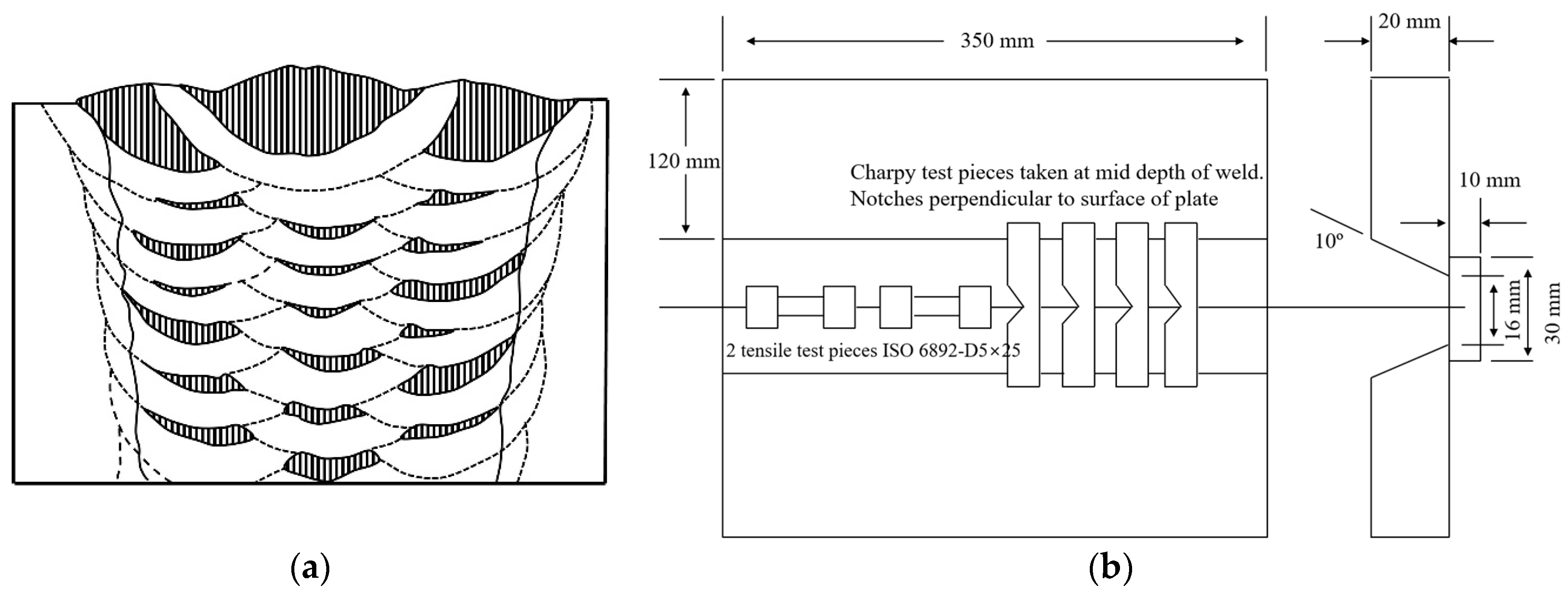
2.1. Data Collection

In this study, experimental data were extracted from Evans and Bailey [1] to understand changes in the mechanical properties with respect to the chemical composition. Mn, which is known to improve the strength significantly, was used as the base. Next, results of experiments on the yield strength, tensile strength, and impact toughness according to the increase in the content of each alloying element were analyzed. To evaluate the impact toughness, the Charpy V-notch (CVN) transition temperature at 100 J was applied, hereinafter referred to as the CVN temperature.

Figure 1a,b shows the shape of the weld used in this study and the sampling method of the specimen. Shielded metal arc welding (SMAW) was applied as the welding technique. The base material and the electrode were welded by using the arc heat generated between a coated electrode and a metal. Herein, ISO 2560:2020, the welding standard for mild steel and low-alloy steel, was applied [16].

The welding electrode was manufactured using the standard technique for a 25% iron powder-coated electrode, and all components were kept constant, except for the components used in the investigation. The automatic spectrographic (ICP-AES) technique was applied for chemical composition analysis. All the core wires of the welding electrode had similar typical compositions of 0.07 C, 0.50 Mn, 0.008 Si, 0.006 S, 0.008 P, 0.02 Cr, 0.003 Mo, 0.03 Ni, 0.02 Cu, 0.0004 Ti, 0.0015 Al, 0.0005 Nb, 0.0005 V, 0.0002 B, 0.02 O, and 0.0025 N (wt%).

The weldment was performed in three beads per layer, as shown in Figure 1a. Two 20 mm-thick mild steel plates were attached to a backing strip, and a jig in a flat (downhand) position with a stringer bead was welded. The root gap size was designed to be 16 mm as shown in Figure 1b. Welding conditions were applied such that the current was 170 A, the voltage was 21 V, the interpass temperature was maintained at 200 °C, and the welding speed was adjusted so that the heat input was 1 kJ/mm. For the interpass temperature, the maximum interpass temperature suitable for welding short blocks in ISO 2560:2020 was applied.

The cross section of the panel after welding is shown in Figure 1b. The mechanical properties were tested under ‘as-welded’ conditions, and the specimens for tensile testing were heated at 250 °C for 14 h to remove diffusive hydrogen. Duplicate tests were conducted with ISO 6892 standard specimens using a gauge with a length of 500 mm and a diameter of 5 mm in a direction parallel to the welding direction.

In the case of metals, the fracture behavior varies from ductile to brittle as the temperature changes from high to low. This change in the fracture mode depends on the material ability to absorb fracture energy. Evans and Bailey [1] conducted an impact toughness test using a CVN impact test, and the specimen was manufactured by machining an axis perpendicular to the welding direction and a notch perpendicular to the plate surface, as shown in Figure 1b. The CVN impact test followed the E23 test procedure of the American Society for Testing Materials (ASTM). Figure 2 shows a typical CVN impact energy curve with respect to the temperature. As shown in Figure 2, the curve is divided into three regions: the upper shelf, lower shelf, and transition. The upper shelf region is a ductile region, the lower shelf is a brittle region, and the transition region is a reference temperature for defining the failure mode as the DBTT. The Charpy impact toughness is generally evaluated based on the transition temperature when absorbing 28 J and 100 J impact energies. In this study, we applied only 100 J of impact energy from a conservative point of view. The 100 J transition temperature data used in this study were obtained from the impact energy and temperature curves obtained through 36 impact tests for each composition condition.

Table 1. Composition of the weld metal with varying alloy and Mn contents data adapted from [1].

Mn	C	Si	Cr	Ni	Mo	O	V	Nb
0.6	0.04	0.20	0.25	0.50	0.0	0.03	0.0004	0.0004
	0.06	0.40	0.50	1.0	0.25	0.037	0.02	0.01
	0.10	0.60	1.0	2.25	0.50	0.045	0.04	0.02
	0.15	0.90	2.3	3.5	1.1	-	0.06	0.045
	-	-	-	-	-	-	0.08	0.09
1.0	0.04	0.20	0.25	0.50	0.0	0.03	0.0004	0.0004
	0.06	0.40	0.50	1.0	0.25	0.037	0.02	0.01
	0.10	0.60	1.0	2.25	0.50	0.045	0.04	0.02
	0.15	0.90	2.3	3.5	1.1	-	0.06	0.045
	-	-	-	-	-	-	0.08	0.09
	0.04	0.20	0.25	0.50	0.0	0.03	0.0004	0.0004
	0.06	0.40	0.50	1.0	0.25	0.037	0.02	0.01
1.4	0.10	0.60	1.0	2.25	0.50	0.045	0.04	0.02
	0.15	0.90	2.3	3.5	1.1	-	0.06	0.045
	-	-	-	-	-	-	0.08	0.09
	0.04	0.20	0.25	0.50	0.0	0.03	0.0004	0.0004
	0.06	0.40	0.50	1.0	0.25	0.037	0.02	0.01
1.8	0.10	0.60	1.0	2.25	0.50	0.045	0.04	0.02
	0.15	0.90	2.3	3.5	1.1	-	0.06	0.045
	-	-	-	-	-	-	0.08	0.09

shows the composition of the weld metal with varying alloy and Mn content used in this study. Nominal Mn contents of 0.6%, 1.0%, 1.4%, and 1.8% were used, and for each Mn content, three to five varying contents of each element were tested.

Table 2. Typical composition except for the elements under investigation data adapted from [1].

	C	Si	Cr	Ni	Mo	O	V	Nb	S	P	N	Cu	Ti	Al	B
Mn–C	-	0.30	0.03	0.03	0.005	0.049	0.012	0.002	0.006	0.013	0.007	0.03	0.0055	0.0005	0.0002
Mn–Si	0.066	-	0.03	0.03	0.005	0.04	0.012	0.002	0.006	0.013	0.006	0.03	0.0055	0.0005	0.0002
Mn–Cr	0.046	0.32	-	0.03	0.005	0.04	0.012	0.002	0.006	0.013	0.006	0.03	0.0055	0.0005	0.0002
Mn–Ni	0.045	0.32	0.03	-	0.005	0.04	0.012	0.002	0.006	0.013	0.006	0.03	0.0055	0.0005	0.0002
Mn–Mo	0.043	0.33	0.03	0.03	-	0.04	0.012	0.002	0.006	0.013	0.006	0.03	0.0055	0.0005	0.0002
Mn–O	0.078	0.32	0.03	0.03	0.005	-	0.012	0.002	0.006	0.008	0.007	0.03	0.0005	0.0005	0.0002
Mn–V	0.076	0.31	0.03	0.03	0.005	0.042	-	0.0006	0.007	0.006	0.008	0.03	0.0032	0.0005	0.0002
Mn–Nb	0.076	0.32	0.03	0.03	0.005	0.042	0.0007	-	0.007	0.006	0.009	0.03	0.0036	0.0005	0.0002

shows typical compositions, except for the elements under investigation.

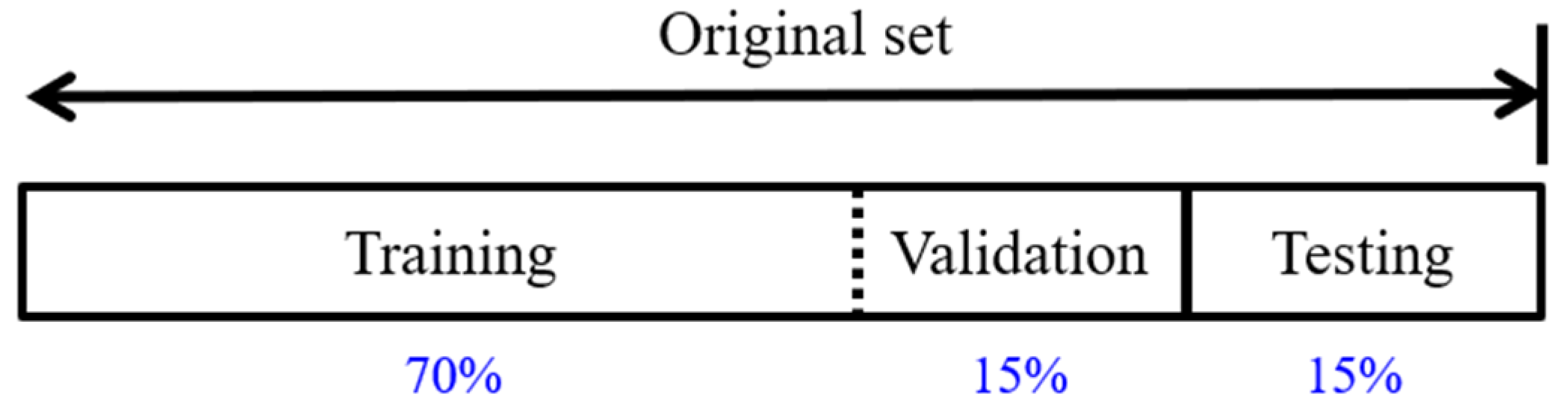
2.2. Data Augmentation

A sufficiently large dataset is required for accurately determining the relationship between the input and the output because the ANN is a data-driven approach. However, the amount of publicly available data on changes in mechanical properties with respect to weld chemical composition is small. Although experiments have been conducted in a large number of studies, it is difficult to create a single dataset owing to different welding methods and conditions. Although the data by Evans and Bailey [1] applied in this study are relatively diverse and provide many experimental results, the amount of data for individual experiments is still insufficient, which may lead to inaccurate predictions. Therefore, in this study, the amount of initial input data was increased by applying a data augmentation technique.

Figure 3 shows an example of the data augmentation applied in this study. There are only four Mn test data points for the 0.04 C condition. Because the amount of data is small and the trends are different, training the ANN directly may cause an inaccurate fitting or overfitting. Therefore, the test data (asterisks in Figure 3) were first plotted for each condition, and then, nonlinear regression was performed with a line that expressed the test data as good as possible. Finally, ten additional data points (circles in Figure 3) were added to the regression line. Although scatter exists owing to the nature of the experimental data, it is expected that a predictive model with better performance can be generated because the finely tuned data after direct fitting are used for model training.

3. Development of Closed-Form Equations Using the ANN Model

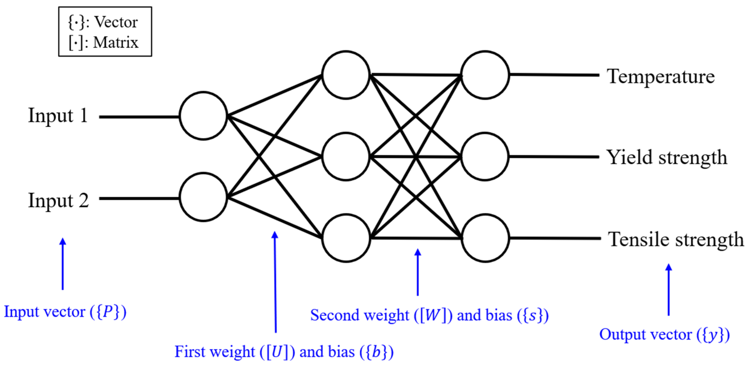
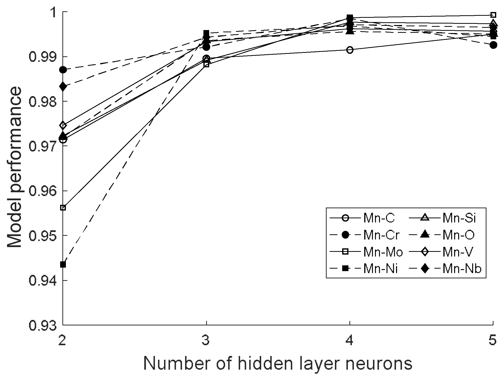
3.1. ANN Model

As shown in Table 1, in this study, we intended to create ANN models that can predict mechanical properties of welds using two variables (chemical compositions). If only one output is obtained from two inputs, multivariate nonlinear regression can be applied because it can be expressed in three dimensions. However, it is difficult to use the existing statistical method to create a model that calculates three outputs (yield strength, tensile strength, and 100 J Charpy temperature) simultaneously. Therefore, it is required to apply the ANN, which is a machine-learning approach that can effectively express multivariate nonlinear systems. The ANN has no limit to the number of input or output variables. If an appropriate structure is used, multiple outputs can be simultaneously derived from multiple inputs.

Figure 4 shows the structure of the ANN model used in this study. This neural network had one input layer, one hidden layer, and one output layer. In the figure, the circle represents the node constituting each layer, and the connecting line represents the weight and the bias representing the relationship between each node. Two input vectors (for example, the content of Mn and the content of C) are fed into the input layer and the output vectors (yield strength, tensile strength, and 100 J Charpy transition temperature) are fed into the output layer. Weights and biases between each node are calculated according to the predetermined ANN model structure. Because the number of hidden layer nodes determines the nonlinearity of the entire system, it should be optimized for the corresponding system. That is, too few nodes result in high computation speed but poor accuracy, and many nodes can lead to overfitting and slow computation.

In this study, the number of nodes in the hidden layer was determined using a case study, as shown in Figure 5. For each model, from two to five hidden layer nodes were tested based on the prediction performance. It was observed that the results almost converged if the number of hidden layer nodes exceeded two. Therefore, in consideration of efficiency, three nodes were selected for the hidden layer. The prediction performance was evaluated using the Pearson correlation coefficient between the predicted and target values. That is, the closer it is to one, the better the prediction result.

Equation (1) presents the ANN model applied in this study in the matrix form: ‘tanh’ was used as the activation function for the nonlinearity of the model and the backpropagation algorithm was applied for weight and bias optimization. For the calculation efficiency, all values applied to the calculation were normalized between −1 and 1, as in Equation (2). Therefore, the final derived outputs should be denormalized using Equation (1).

$$\left\{y\right\}=\left\{s\right\}+{\left[W\right]}^{T}tanh\left(\left[U\right]\left\{P\right\}+\left\{b\right\}\right),$$

(1)

$$X_N=2\times \left[\frac{X_R-X_{min}}{X_{max}-X_{min}}\right]-1,$$

(2)

where $X_N$ is the normalized value and $X_R$ is the original value. $X_{max}$ and $X_{min}$ are the maximum and minimum values of $X_R$, respectively.

To evaluate the performance of the trained model, 15% of the original dataset was used as a test dataset. That is, 85% of the total dataset was used for model training and 15% was used for model evaluation. Moreover, out of 85%, 15% was again separated and used for model validation to prevent data overfitting [18]. In summary, the original dataset was divided into training, validation, and testing sets, as illustrated in Figure 6.

Figure 7a,b shows the model performances at the training and testing stages in the Mn–C model, respectively, and Figure 7c presents the performance after combing these two stages. Here, the x-axis represents the target value, and the y-axis represents the predicted value. R represents the Pearson correlation coefficient.

Table 3. Tested R value for each model.

Mn–C	Mn–Si	Mn–Cr	Mn–Ni	Mn–Mo	Mn–O	Mn–V	Mn–Nb
0.98959	0.98922	0.99215	0.99525	0.98821	0.99358	0.99334	0.99430

shows R values for all models. As a result, it can be seen that all models show high prediction accuracy.

3.2. Closed-Form Equations

The previous section discussed the ANN model development for predicting the mechanical properties according to changes in the content of Mn and other compositions. Developing an ANN model is the process of deriving the connection between each node, that is, weight and bias, as shown in Equation (1), through the ‘learning’ process based on the given data. Therefore, it is possible to use Equation (1) with the calculated weights and biases as a closed-form equation. We prepared the ANN models for each case derived in this study using Equation (3). The models for all eight cases, as summarized in Table 1, are presented in the matrix form. For example, n = 1 represents a model for Mn–C, and n = 2 represents Mn–Cr. To calculate the CVN temperature, yield strength, and tensile strength according to the Mn–C content, the Mn and C contents are entered into the P₁ vector. Each value of the y₁ vector is then calculated through a matrix operation. However, because these values are normalized, as mentioned in Section 3.1, the input values should be normalized first before applying Equation (3). The values required for normalization are listed in

Table 4. Reference values for normalization and denormalization.

		Min. Value	Max. Value	Unit
Mn		0.6	1.8	wt%
C		0.04	0.15	wt%
Si		0.2	0.9	wt%
Cr		0.25	2.3	wt%
Ni		0.5	3.5	wt%
Mo		0	1.1	wt%
O		0.03	0.045	wt%
V		0.0004	0.08	wt%
Nb		0.0004	0.09	wt%
Mn–C	Temp.	−64.91	−16.29	°C
	YS	389	626	MPa
	TS	435	711.67	MPa
Mn–Si	Temp.	−66.25	−2.56	°C
	YS	364	587	MPa
	TS	427	665	MPa
Mn–Cr	Temp.	−53.31	33.19	°C
	YS	416	743	MPa
	TS	482	797	MPa
Mn–Ni	Temp.	−62.62	69.39	°C
	YS	391	589	MPa
	TS	458	683	MPa
Mn–Mo	Temp.	−54.93	16.16	°C
	YS	372	736	MPa
	TS	430	796	MPa
Mn–O	Temp.	−65.47	25.86	°C
	YS	378	468	MPa
	TS	467	560	MPa
Mn–V	Temp.	−69.74	−21.27	°C
	YS	366	648	MPa
	TS	459	685	MPa
Mn–Nb	Temp.	−66.45	15.50	°C
	YS	384	682	MPa
	TS	475	729	MPa

. The final calculated y₁ must be denormalized again to convert it to the original scale.

$$\left\{y_n\right\}=\left\{s_n\right\}+{\left[W_n\right]}^{T}tanh\left(\left[U_n\right]\left\{P_n\right\}+\left\{b_n\right\}\right),n=1~8$$

(3)

$$\begin{array}{l}\left\{y_1\right\}=\left\{\begin{array}{c}{\mathrm{Temp}}_{\mathrm{MnC}}\\ {\mathrm{YS}}_{\mathrm{MnC}}\\ {\mathrm{TS}}_{\mathrm{MnC}}\end{array}\right\},\left\{s_1\right\}=\left\{\begin{array}{c}1.049636\\ 0.233576\\ 0.241714\end{array}\right\}, \left[W_1\right]=\left[ {\begin{array}{c}1.010525\\ -0.284486\\ -0.406651\end{array}}^{ }{\begin{array}{c} 0.635715\\ 1.199921\\ 1.102196\end{array}}^{ }{\begin{array}{c} 0.773552\\ -0.18018\\ -0.02591\end{array}}^{ } \right],\\ \left[U_1\right]=\left[{\begin{array}{c}-0.86956\\ 0.51526\\ -1.05571\end{array}}^{ }{\begin{array}{c}-0.64436\\ 0.45486\\ 0.46409\end{array}}^{ }\right],\left\{P_1\right\}=\left\{ \begin{array}{c}\mathrm{Mn}\\ \mathrm{C}\end{array} \right\},\left\{b_1\right\}=\left\{\begin{array}{c}-0.93884\\ -0.69465\\ -0.66777\end{array}\right\}\end{array}$$

$$\begin{array}{l}\left\{y_2\right\}=\left\{\begin{array}{c}{\mathrm{Temp}}_{\mathrm{MnCr}}\\ {\mathrm{YS}}_{\mathrm{MnCr}}\\ {\mathrm{TS}}_{\mathrm{MnCr}}\end{array}\right\}, \left\{s_2\right\}=\left\{\begin{array}{c}1.311486\\ -0.06367\\ -0.05746\end{array}\right\}, \left[W_2\right]=\left[ {\begin{array}{c}1.872796\\ 0.000750\\ 0.004089\end{array}}^{ }{\begin{array}{c} 0.87106\\ -0.014840\\ -0.000017\end{array}}^{ }{\begin{array}{c}-2.98703\\ 3.639551\\ 3.643273\end{array}}^{ } \right],\\ \left[U_2\right]=\left[{\begin{array}{c}1.186769\\ -1.36505\\ 0.163576\end{array}}^{ }{\begin{array}{c} 0.603857\\ 0.914433\\ 0.113679\end{array}}^{ }\right],\left\{P_2\right\}=\left\{\begin{array}{c}\mathrm{Mn}\\ \mathrm{Cr}\end{array}\right\},\left\{b_2\right\}=\left\{\begin{array}{c}-0.92949\\ -0.71739\\ 0.016649\end{array}\right\}\end{array}$$

$$\begin{array}{l}\left\{y_3\right\}=\left\{\begin{array}{c}{\mathrm{Temp}}_{\mathrm{MnNi}}\\ {\mathrm{YS}}_{\mathrm{MnNi}}\\ {\mathrm{TS}}_{\mathrm{MnNi}}\end{array}\right\},\left\{s_3\right\}=\left\{\begin{array}{c}1.951395\\ -0.02477\\ -0.99595\end{array}\right\},\left[W_3\right]=\left[ {\begin{array}{c}1.72015\\ -0.55666\\ -0.75407\end{array}}^{ }{\begin{array}{c}-0.25232\\ -1.45942\\ -0.81762\end{array}}^{ }{\begin{array}{c}-2.50412\\ -0.39684\\ -0.54086\end{array}}^{ } \right],\\ \left[U_3\right]=\left[{\begin{array}{c}-0.63435\\ -0.34123\\ -0.77397\end{array}}^{ }{\begin{array}{c}-0.28357\\ 0.025948\\ -0.35558\end{array}}^{ }\right],\left\{P_3\right\}=\left\{\begin{array}{c}\mathrm{Mn}\\ \mathrm{Ni}\end{array} \right\},\left\{b_3\right\}=\left\{\begin{array}{c}-0.69519\\ 0.014862\\ 0.921754\end{array}\right\}\end{array}$$

$$\begin{array}{l}\left\{y_4\right\}=\left\{\begin{array}{c}{\mathrm{Temp}}_{\mathrm{MnSi}}\\ {\mathrm{YS}}_{\mathrm{MnSi}}\\ {\mathrm{TS}}_{\mathrm{MnSi}}\end{array}\right\},\left\{s_4\right\}=\left\{\begin{array}{c}0.024837\\ -0.01735\\ 0.168692\end{array}\right\},\left[W_4\right]=\left[ {\begin{array}{c}1.039145\\ -0.22634\\ -0.01153\end{array}}^{ }{\begin{array}{c}-0.09436\\ -1.59469\\ -2.00920\end{array}}^{ }{\begin{array}{c} 0.047961\\ -0.35168\\ -0.17194\end{array}}^{ } \right],\\ \left[U_4\right]=\left[{\begin{array}{c}-1.08566\\ -0.32260\\ -0.32434\end{array}}^{ }{\begin{array}{c} 0.581902\\ -0.14604\\ -1.23222\end{array}}^{ }\right],\left\{P_4\right\}=\left\{\begin{array}{c}\mathrm{Mn}\\ \mathrm{Si}\end{array}\right\},\left\{b_4\right\}=\left\{\begin{array}{c}-0.38397\\ 0.140286\\ -1.27282\end{array}\right\}\end{array}$$

$$\begin{array}{l}\left\{y_5\right\}=\left\{\begin{array}{c}{\mathrm{Temp}}_{\mathrm{MnMo}}\\ {\mathrm{YS}}_{\mathrm{MnMo}}\\ {\mathrm{TS}}_{\mathrm{MnMo}}\end{array}\right\},\left\{s_5\right\}=\left\{\begin{array}{c}1.057515\\ -0.03976\\ -0.03826\end{array}\right\},\left[W_5\right]=\left[ {\begin{array}{c}-0.99300\\ -0.78631\\ -0.85297\end{array}}^{ }{\begin{array}{c}-1.49291\\ 0.499370\\ 0.472669\end{array}}^{ }{\begin{array}{c} 1.051739\\ 0.429281\\ 0.406191\end{array}}^{ } \right],\\ \left[U_5\right]=\left[{\begin{array}{c}-0.03755\\ 0.992052\\ 1.084931\end{array}}^{ }{\begin{array}{c}-0.49507\\ 0.111495\\ 0.121627\end{array}}^{ }\right],\left\{P_5\right\}=\left\{\begin{array}{c}\mathrm{Mn}\\ \mathrm{Mo}\end{array} \right\},\left\{b_5\right\}=\left\{\begin{array}{c}-0.00999\\ 0.779431\\ -0.82102\end{array}\right\}\end{array}$$

$$\begin{array}{l}\left\{y_6\right\}=\left\{\begin{array}{c}{\mathrm{Temp}}_{\mathrm{MnO}}\\ {\mathrm{YS}}_{\mathrm{MnO}}\\ {\mathrm{TS}}_{\mathrm{MnO}}\end{array}\right\},\left\{s_6\right\}=\left\{\begin{array}{c}1.077799\\ 0.067542\\ 0.067552\end{array}\right\},\left[W_6\right]=\left[ {\begin{array}{c}2.043723\\ 0.768526\\ 0.768559\end{array}}^{ }{\begin{array}{c}-0.59919\\ 1.142815\\ 1.142852\end{array}}^{ }{\begin{array}{c}-0.19960\\ 0.213232\\ 0.213249\end{array}}^{ } \right],\\ \left[U_6\right]=\left[{\begin{array}{c}1.049968\\ 0.833696\\ -0.13802\end{array}}^{ }{\begin{array}{c} 0.121991\\ 0.110389\\ -0.71512\end{array}}^{ }\right],\left\{P_6\right\}=\left\{ \begin{array}{c}\mathrm{Mn}\\ \mathrm{O}\end{array} \right\},\left\{b_6\right\}=\left\{\begin{array}{c}-1.08092\\ 0.556272\\ -0.18993\end{array}\right\}\end{array}$$

$$\begin{array}{l}\left\{y_7\right\}=\left\{\begin{array}{c}{\mathrm{Temp}}_{\mathrm{MnV}}\\ {\mathrm{YS}}_{\mathrm{MnV}}\\ {\mathrm{TS}}_{\mathrm{MnV}}\end{array}\right\},\left\{s_7\right\}=\left\{\begin{array}{c}3.559261\\ -0.315284\\ -0.319956\end{array}\right\},\left[W_7\right]=\left[ {\begin{array}{c}1.958502\\ -0.18359\\ -0.22796\end{array}}^{ }{\begin{array}{c}-2.09365\\ 1.548604\\ 1.513895\end{array}}^{ }{\begin{array}{c} 2.507940\\ 0.480616\\ 0.500507\end{array}}^{ } \right],\\ \left[U_7\right]=\left[{\begin{array}{c}-0.81832\\ 0.335151\\ 0.865442\end{array}}^{ }{\begin{array}{c} 0.358623\\ 0.280673\\ 0.267847\end{array}}^{ }\right],\left\{P_7\right\}=\left\{ \begin{array}{c}\mathrm{Mn}\\ \mathrm{V}\end{array} \right\},\left\{b_7\right\}=\left\{\begin{array}{c}-0.94493\\ 0.428865\\ -1.24693\end{array}\right\}\end{array}$$

$$\begin{array}{l}\left\{y_8\right\}=\left\{\begin{array}{c}{\mathrm{Temp}}_{\mathrm{MnNb}}\\ {\mathrm{YS}}_{\mathrm{MnNb}}\\ {\mathrm{TS}}_{\mathrm{MnNb}}\end{array}\right\},\left\{s_8\right\}=\left\{\begin{array}{c}-0.22090\\ -0.31089\\ -0.28607\end{array}\right\},\left[W_8\right]=\left[ {\begin{array}{c}0.769446\\ 0.724100\\ 0.667899\end{array}}^{ }{\begin{array}{c}-1.06027\\ -1.66486\\ -1.79086\end{array}}^{ }{\begin{array}{c} 0.724919\\ -0.02200\\ 0.005047\end{array}}^{ } \right],\\ \left[U_8\right]=\left[{\begin{array}{c}-0.00234\\ -0.29114\\ -1.43752\end{array}}^{ }{\begin{array}{c} 1.101230\\ -0.08185\\ 0.558518\end{array}}^{ }\right],\left\{P_8\right\}=\left\{ \begin{array}{c}\mathrm{Mn}\\ \mathrm{Nb}\end{array} \right\},\left\{b_8\right\}=\left\{\begin{array}{c}1.016240\\ 0.006815\\ -0.26343\end{array}\right\}\end{array}$$

4. Model Performance Estimation and Discussion

The results calculated using the ANN model (Equation (3)) were compared with the original test data to estimate the model performance. Figure 8, Figure 9 and Figure 10 show the comparison between the calculated and experimental results using one of the eight models (Mn–Ni) in terms of 100 J Charpy temperature, yield strength, and tensile strength, respectively. The comparison results for the rest of the models for temperature are shown in Figure A1, Figure A2, Figure A3, Figure A4, Figure A5, Figure A6 and Figure A7 in Appendix A. In the case of yield and tensile strengths, we only included one case (Figure 9 and Figure 10) because all other cases showed a nearly linear relationship and were almost consistent with the experimental results. In the figure, the lines represent the estimation (E), and the symbols represent the tested data (T).

It can be seen that the trend of the fitting results for the experimental results varies greatly depending on the type or content of the ingredients contained. For example, in Figure 8a, the temperature difference is not large depending on the Mn content in 0.5 Ni, and the temperature does not increase even when the Mn content is increased. However, as the Ni content is increased, the temperature increases rapidly with the Mn content, particularly for 3.5 Ni (Figure 8d). As shown in the other figures in the Appendix A, the trends are all different for the other elements. This indicates that the nonlinearity is large, depending on the type or content of the chemical component. In contrast, in terms of yield and tensile strengths, although the slopes are slightly different, they show an almost perfect linear relationship with the Mn content, regardless of the type or content of the component.

As a result, in most cases, the estimated and experimental values show good agreement. However, in some cases, for example, in the case of the CVN temperature of Mn–1.1Mo in Figure A4, an estimation error occurs. This seems to be because, in this case, the experimental results have greater nonlinearity than in the other cases. When the nonlinearity of the data used in the ANN model is high, the fitting accuracy can be improved by increasing the number of hidden layers. However, if the number of hidden layers is increased, there is a risk of overfitting. Therefore, the decision should be made by considering the overall data trend. In the case of the CVN temperature of Mn–1.1Mo, this error seems to be unavoidable because only this case has a large nonlinearity. It is expected that as the amount of experimental data is increased, the accuracy can be increased further. In contrast, for all cases of yield and tensile strengths, the prediction results show high accuracy, as compared with the test results, because the data used for the model training show a strong linearity.

5. Conclusions

In this study, existing experimental data were collected to investigate changes in the following mechanical properties: 100 J Charpy temperature, yield strength, and tensile strength, depending on the chemical composition. Trends were analyzed by applying an ANN to the data. Data augmentation was performed to solve the problem of insufficient data caused by the dependence of experimental results on specific conditions. Finally, closed-form equations were developed based on the coefficients derived from the ANN models to facilitate a prediction. Based on these results, the following conclusions were drawn:

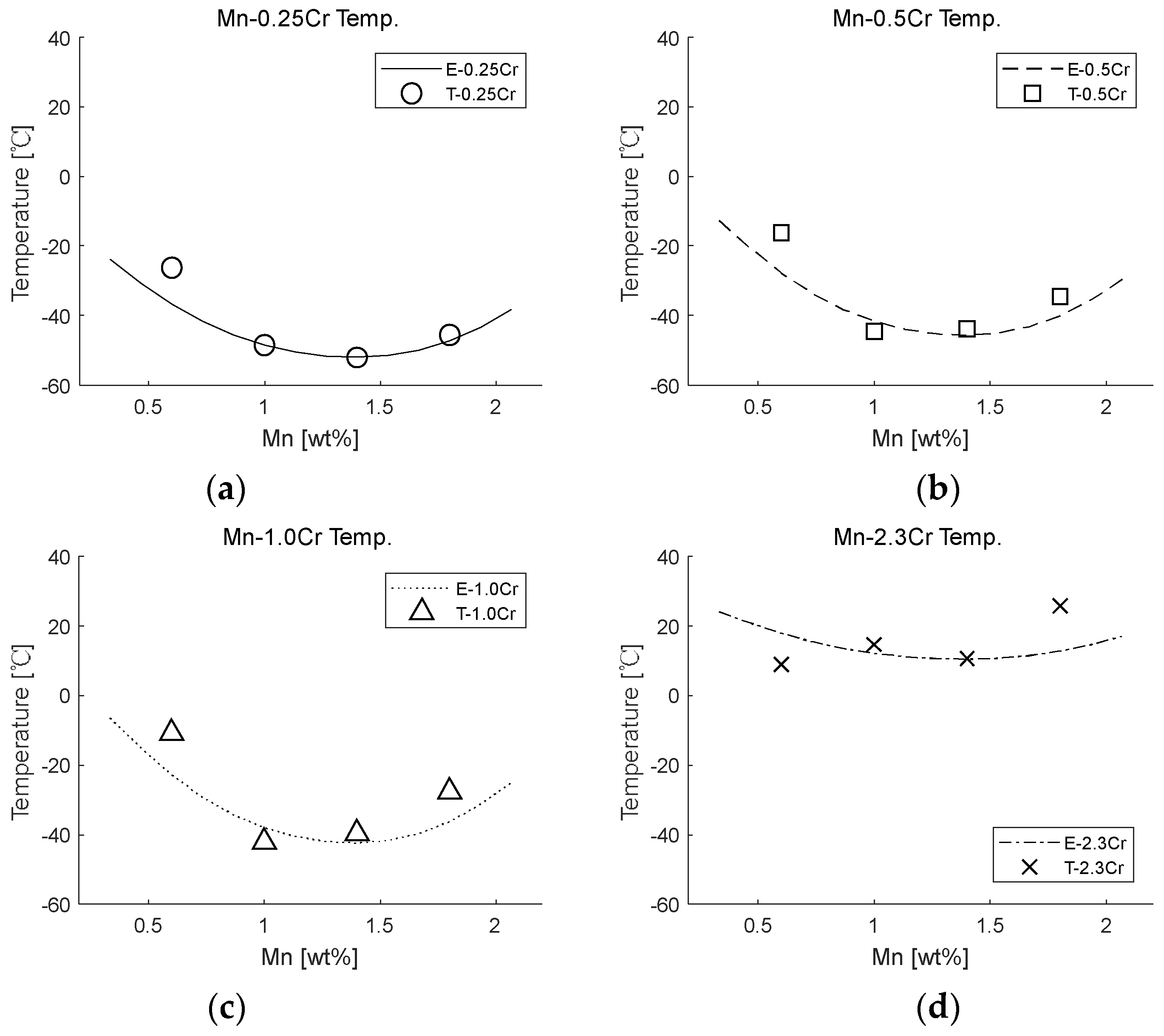
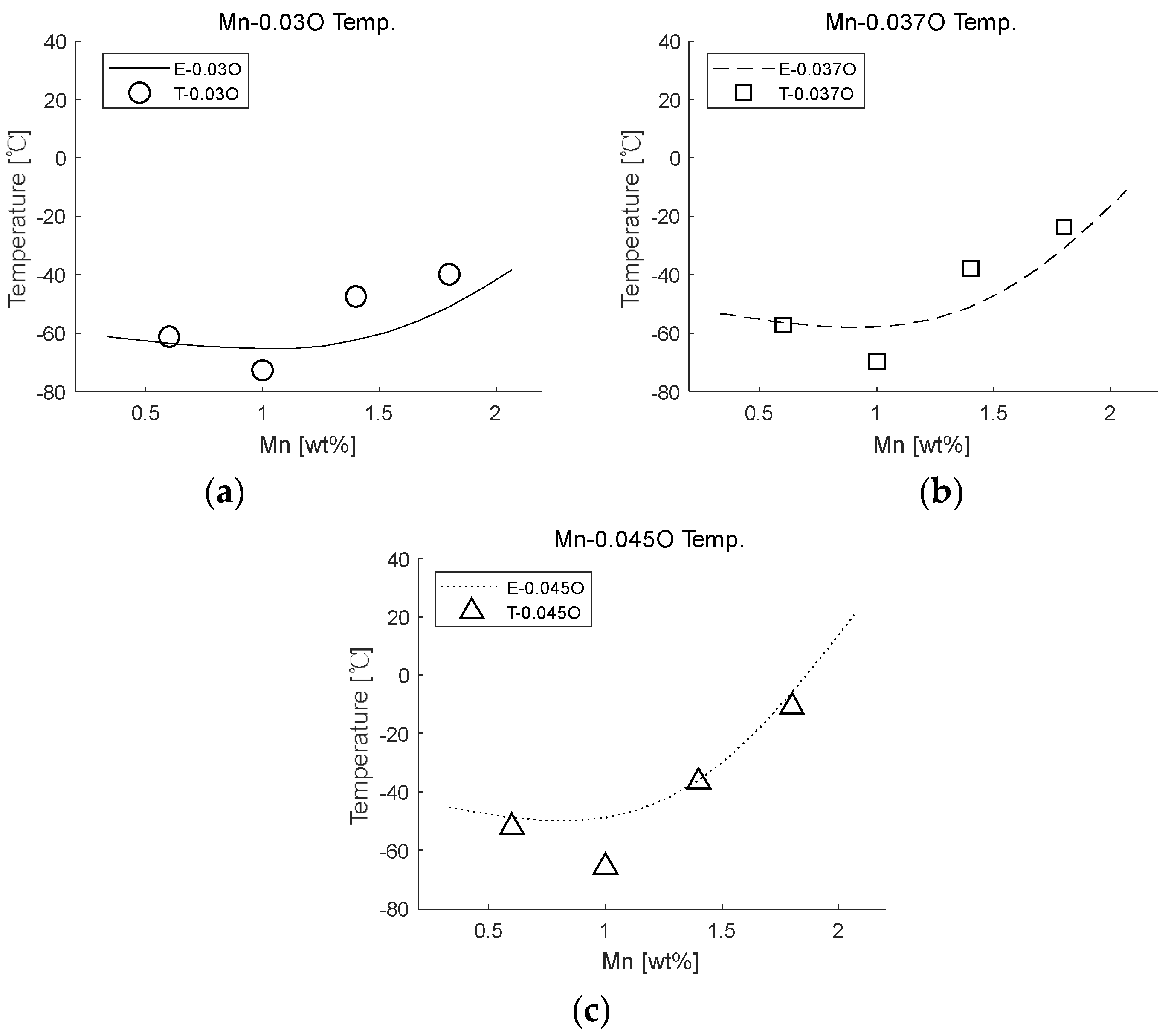
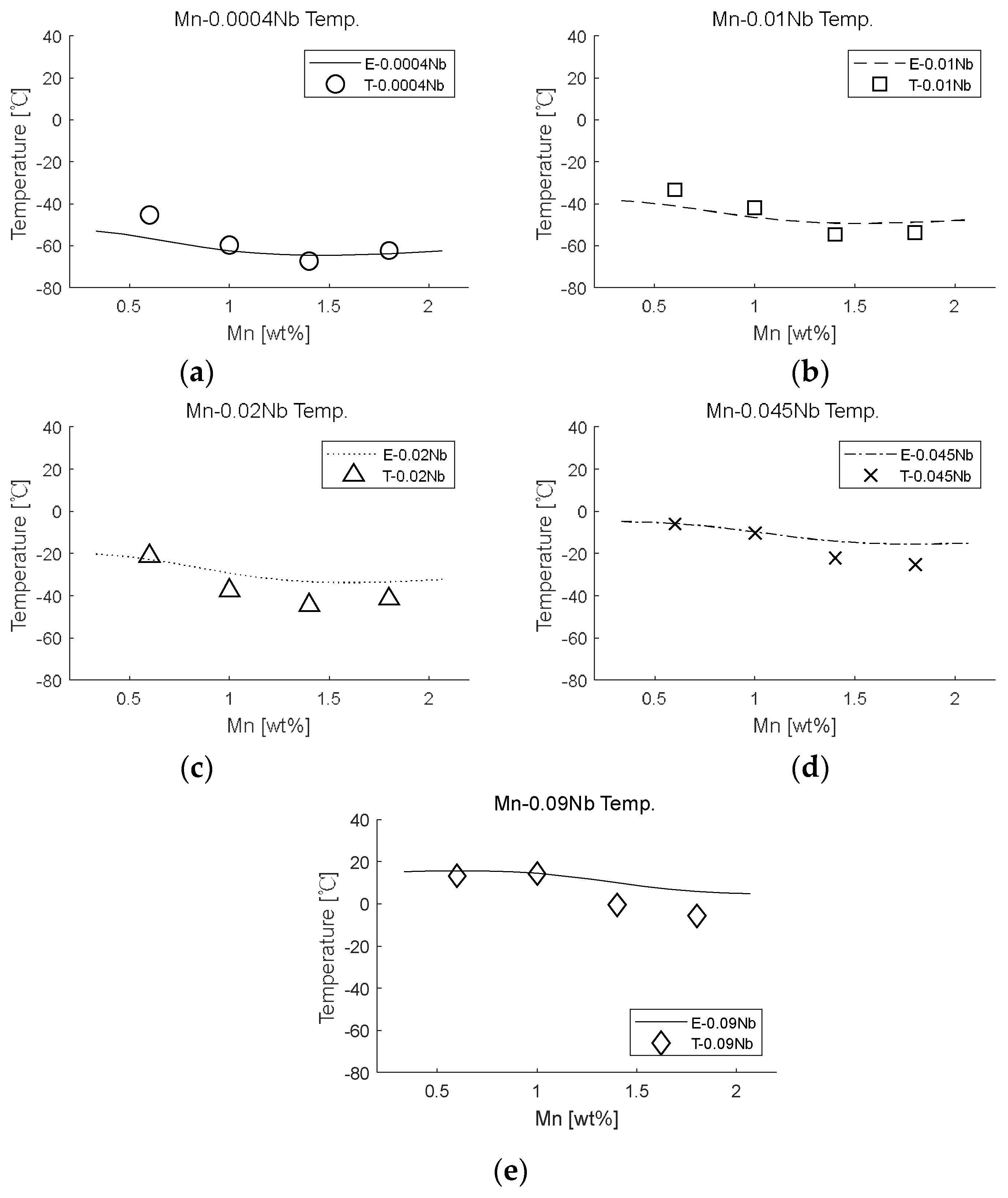
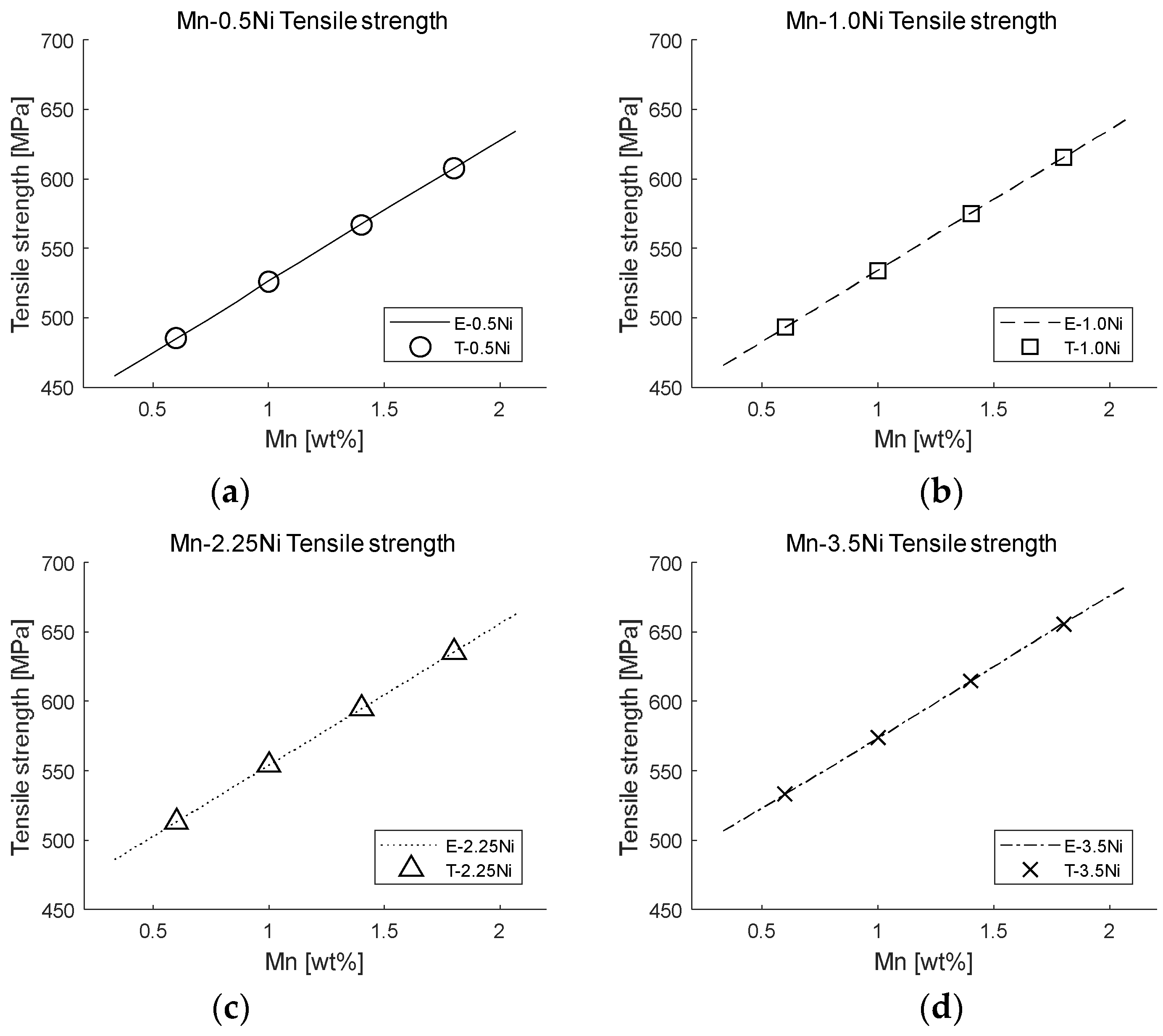
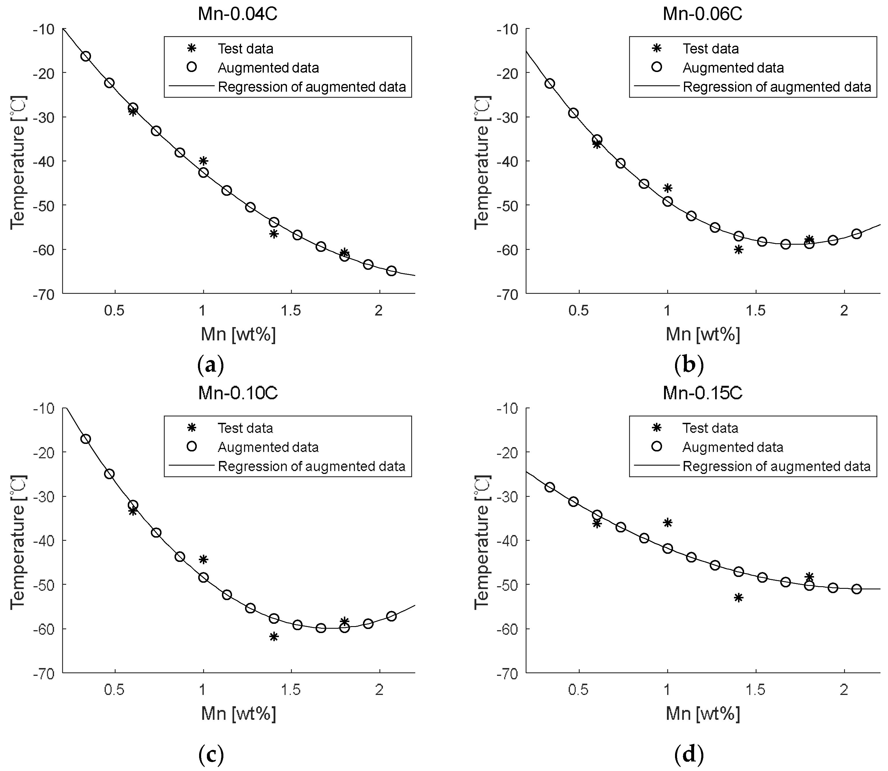
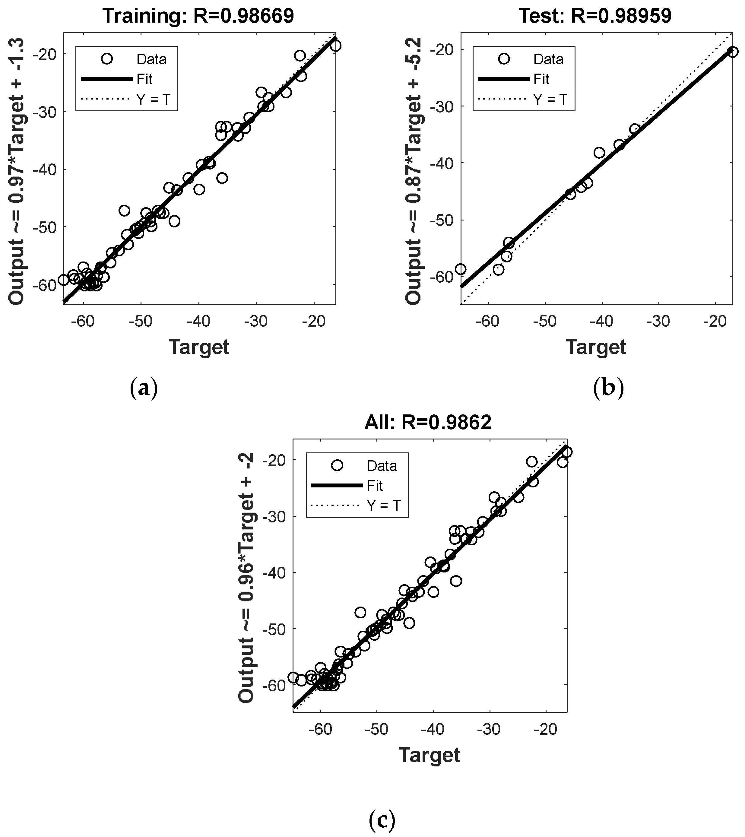
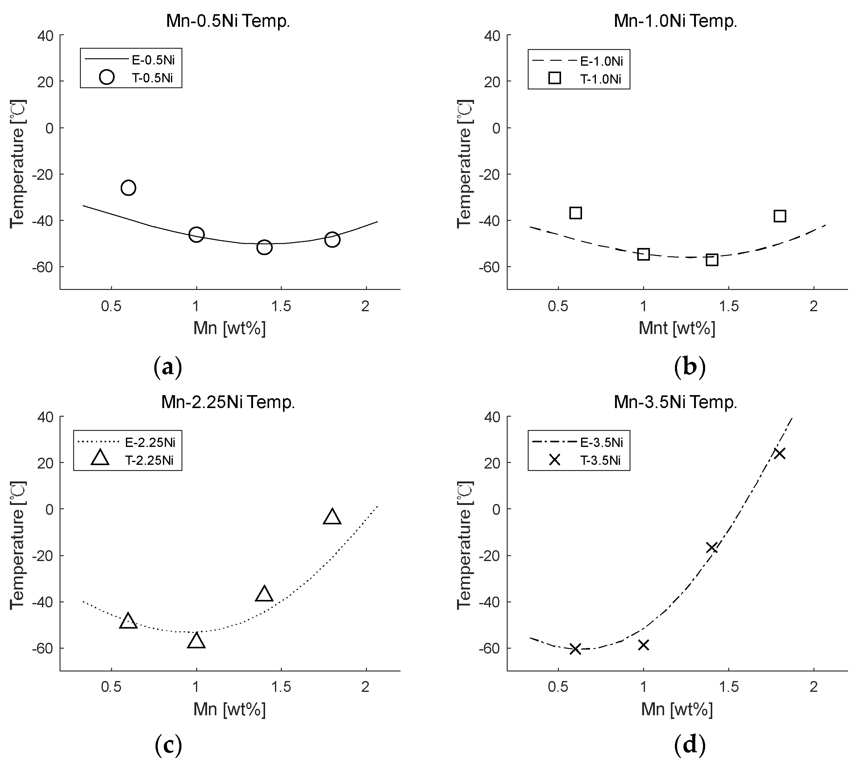
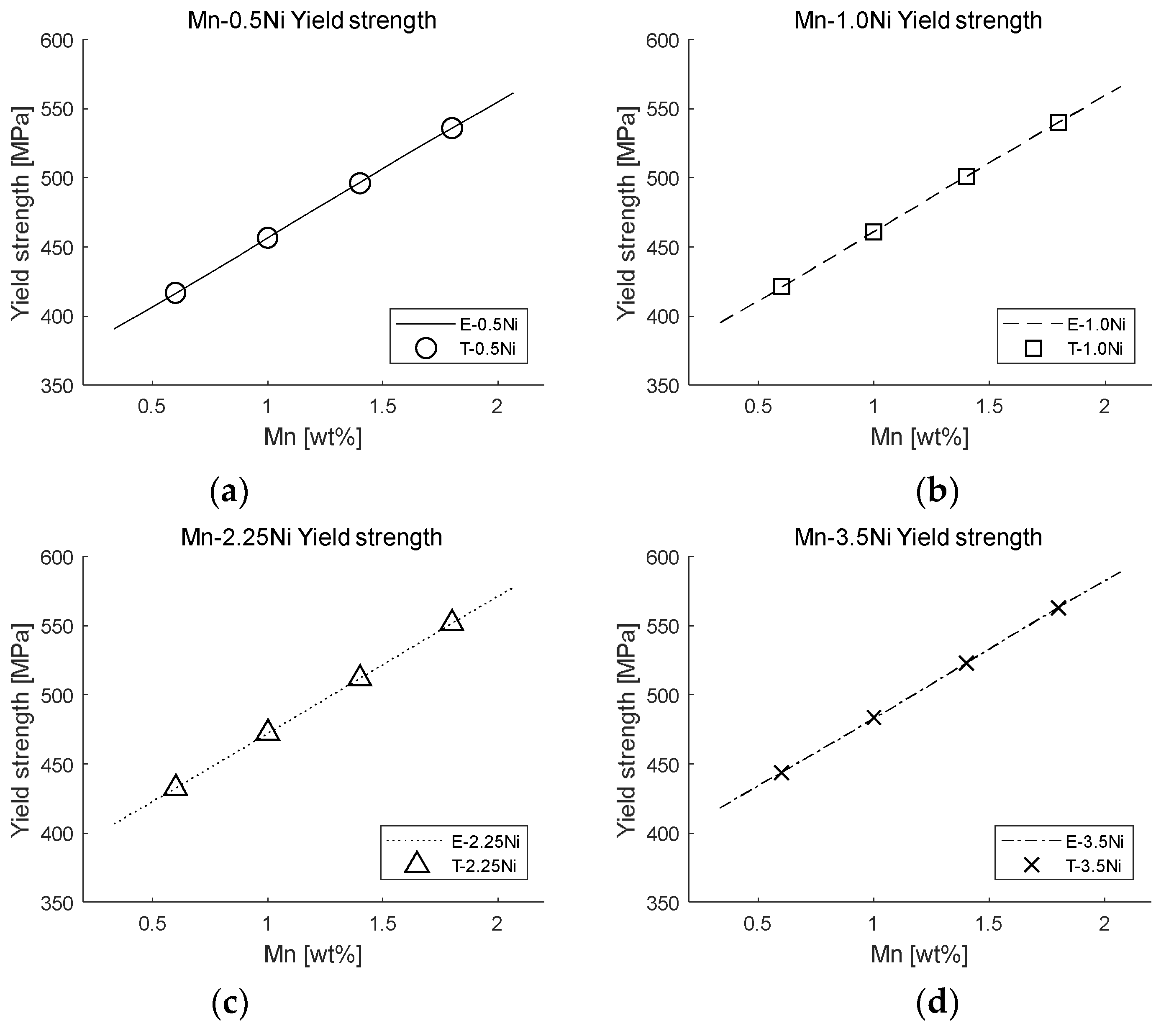
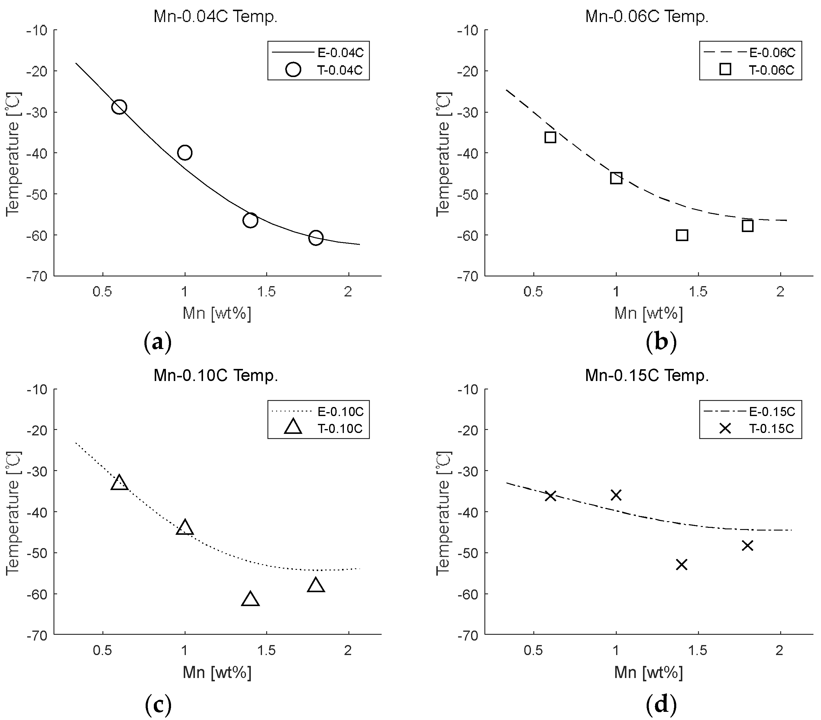
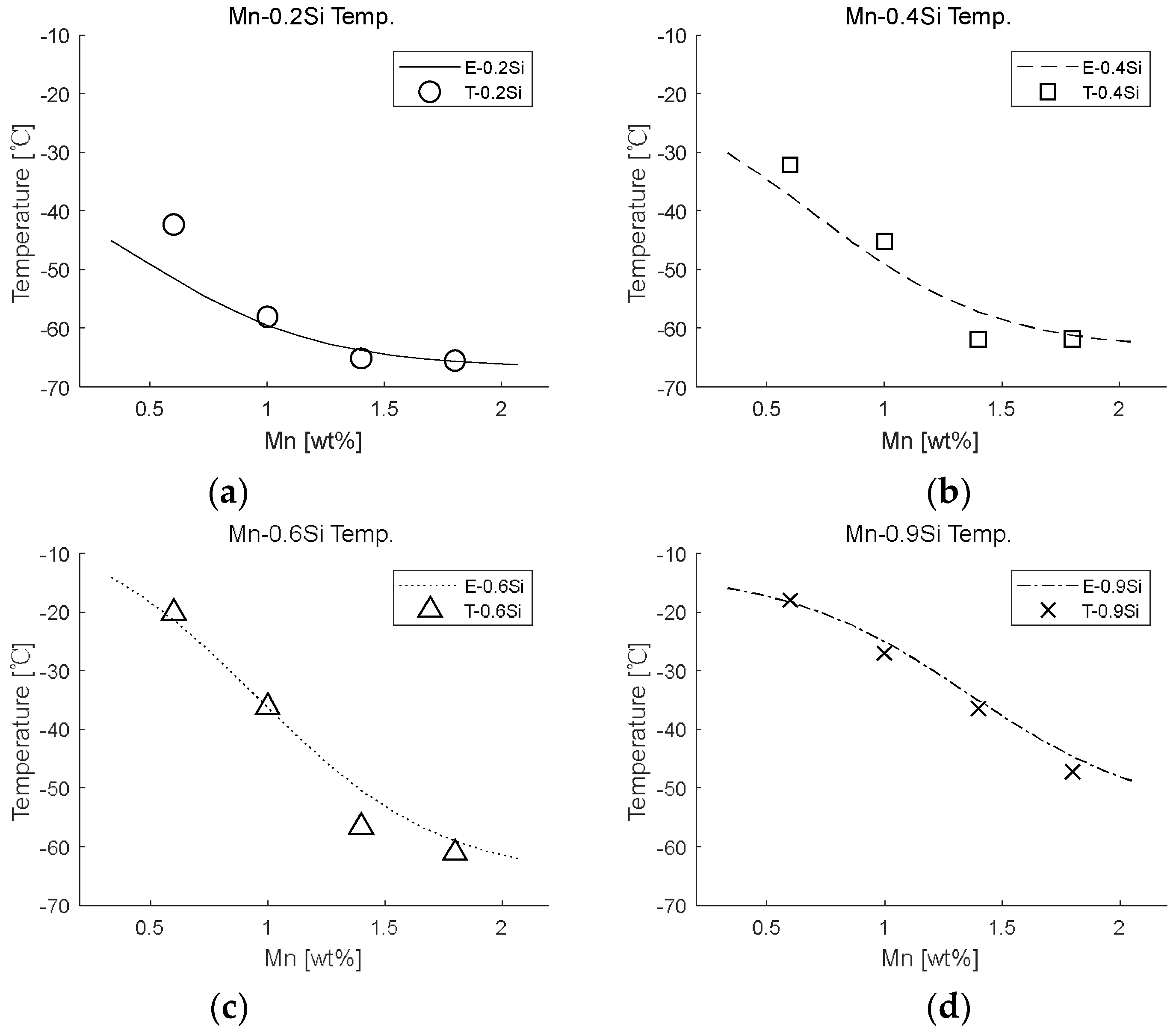
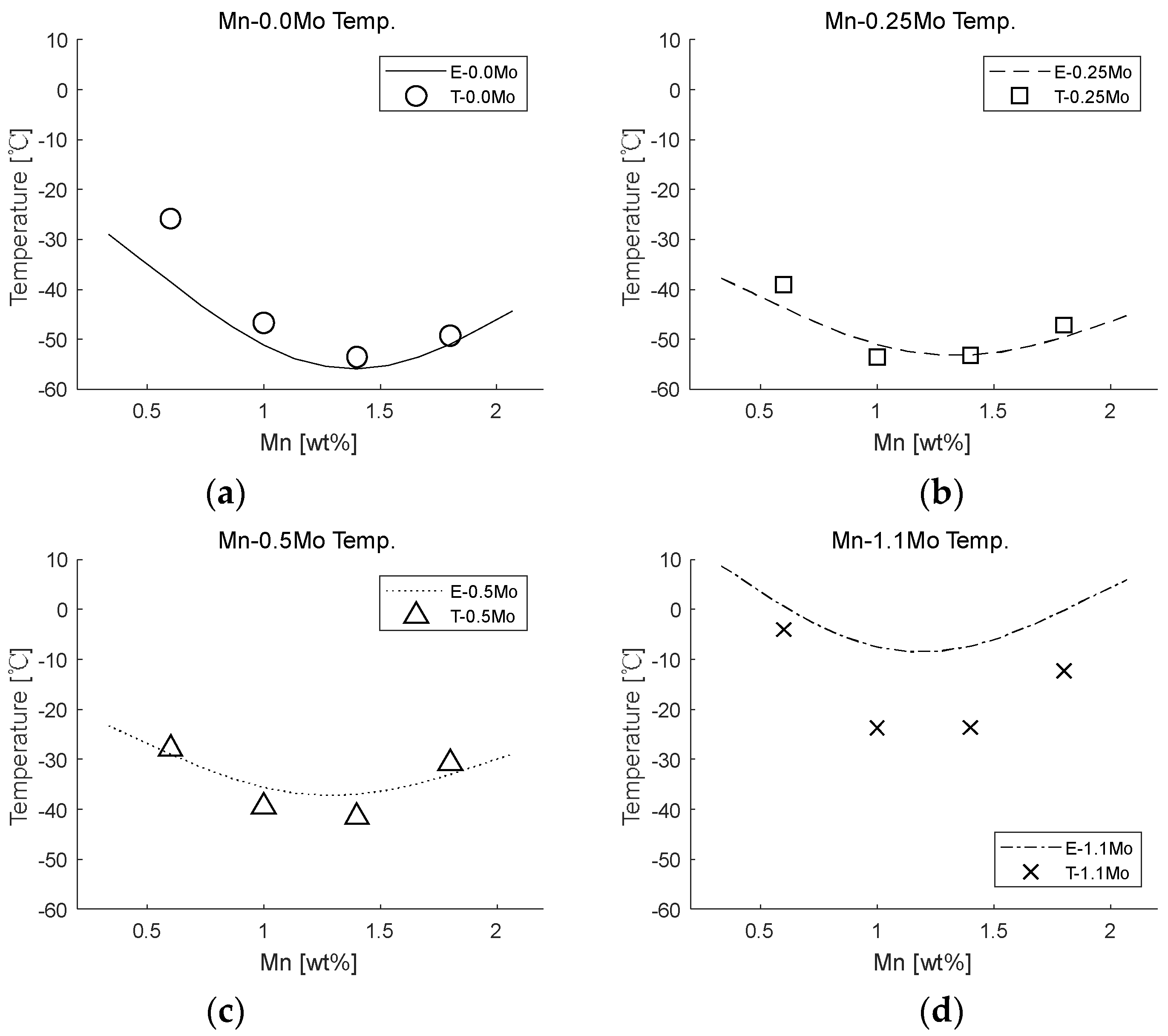
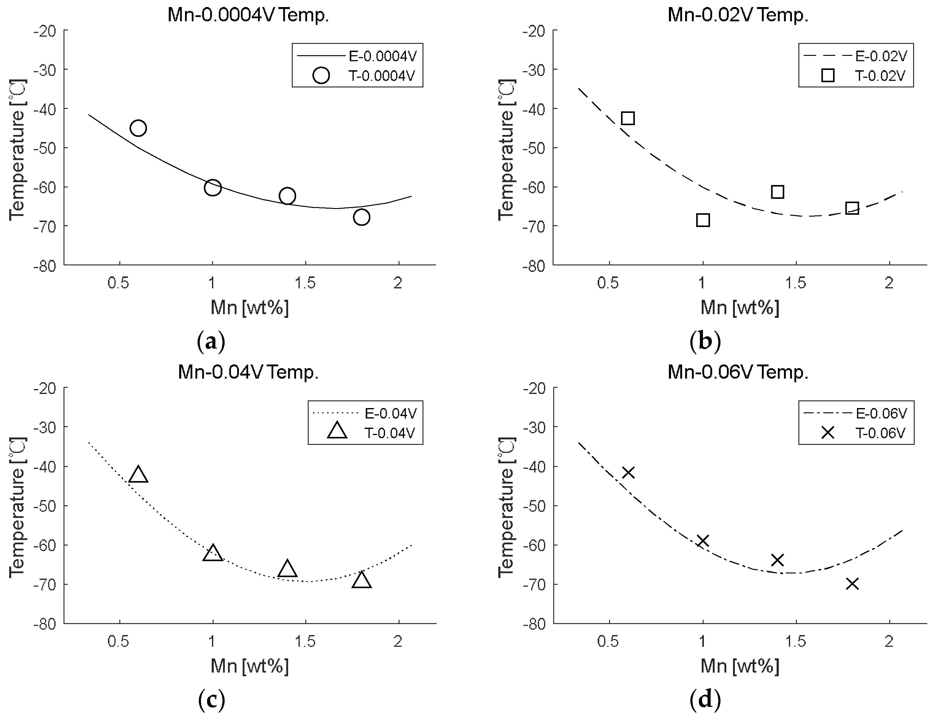
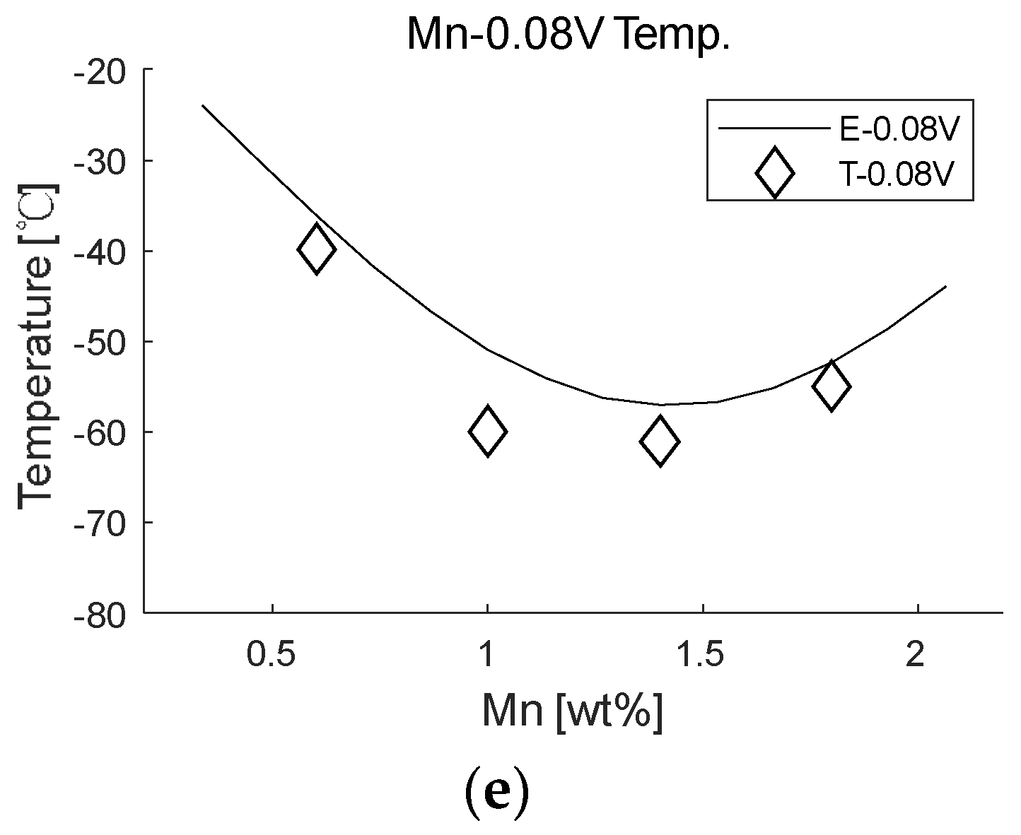
• By increasing the amount of data through data augmentation, the performance of the ANN model improved. Inaccurate regression that may occur due to the insufficient number of experimental results was prevented in advance, and efficient ANN model training was made. However, some cases of CVN temperature showed an estimation error owing to the large nonlinearity in the data used for the ANN training. Because each condition has a different tendency, accurate regression could not be made in this case with relatively large nonlinearity. For a better predictive model, securing more experimental results is essential. In contrast, the yield and tensile strengths showed high accuracy, as the data showed a linear relationship.
• The developed ANN models are presented in the form of vectors and matrices. Therefore, the three mechanical properties considered as targets in this study were calculated by inputting the content of each component through a simple matrix operation.
• However, because each ANN model developed in this study only considered changes in the content of two elements, there is a limitation in that an accurate prediction cannot be performed if any element with a content different from that of the specimen used for the ANN model is included. That is, the results of this study can be mainly used to predict the relative increase or decrease according to the change in the content of two elements, including Mn.
• Further studies are recommended to develop an ANN model based on data collected in a variety of ranges, including other factors. It will then be possible to efficiently estimate the exact mechanical properties with respect to the contents of chemical compositions.

References

1. Evans, G.M.; Bailey, N. Metallurgy of Basic Weld Metal; Woodhead publishing: Sawston, UK, 1997. [Google Scholar]
2. Fleck, N.A.; Grong, Ö.; Edwards, G.R.; Matlock, D.K. The role of filler metal wire and flux composition in submerged arc weld metal transformation kinetics. Weld. J. 1986, 65, 1135–1215. [Google Scholar]
3. Shin, Y.T.; Kang, S.W.; Lee, H.W. Fracture characteristics of TMCP and QT steel weldments with respect to crack length. Mater. Sci. Eng. A 2006, 434, 365–371. [Google Scholar] [CrossRef]
4. Glover, A.G.; McGrath, J.T.; Tinkler, M.J.; Weatherly, G.C. The influence of cooling rate and composition on weld meta microstructures in a C/Mn and a HSLA steel. Simulation 1977, 60, 80. [Google Scholar]
5. Smith, N.J.; McGrath, J.T.; Gianetto, J.A.; Orr, R.F. Microstructure/mechanical property relationships of submerged arc welds in HSLA 80 steel. Weld. J. 1989, 68, 11. [Google Scholar]
6. McGrath, J.T.; Gianetto, J.A.; Orr, R.F.; Letts, M.W. Factors Affecting the Notch Toughness Properties of High Strength HY80 Weldments. Can. Metall. Q. 1986, 25, 349–356. [Google Scholar] [CrossRef]
7. Shao, L.; Ketkaew, J.; Gong, P.; Zhao, S.; Sohn, S.; Bordeenithikasem, P.; Datye, A.; Mota, R.M.O.; Liu, N.; Kube, S.A.; et al. Effect of chemical composition on the fracture toughness of bulk metallic glasses. Materialia 2020, 12, 100828. [Google Scholar] [CrossRef]
8. Balaguru, V.; Balasubramanian, V.; Sivakumar, P. Effect of weld metal composition on impact toughness properties of shielded metal arc welded ultra-high hard armor steel joints. J. Mech. Behav. Mater. 2020, 29, 186–194. [Google Scholar] [CrossRef]
9. Takashima, Y.; Minami, F. Prediction of Charpy absorbed energy of steel for welded structure in ductile-to-brittle fracture transition temperature range. Q. J. Jpn. Weld. Soc. 2020, 38, 103s–107s. [Google Scholar] [CrossRef]
10. Jorge, J.C.F.; Souza, L.; Mendes, M.C.; Bott, I.S.; Araújo, L.S.; Santos, V.; Rebello, J.M.A.; Evans, G.M. Microstructure characterization and its relationship with impact toughness of C–Mn and high strength low alloy steel weld metals—A review. J. Mater. Res. Technol. 2021, 10, 471–501. [Google Scholar] [CrossRef]
11. Khalaj, G.; Pouraliakbar, H.; Mamaghani, K.R.; Khalaj, M.J. Modeling the correlation between heat treatment, chemical composition and bainite fraction of pipeline steels by means of artificial neural networks. Neural Netw. World 2013, 23, 351. [Google Scholar] [CrossRef] [Green Version]
12. Khalaj, G.; Nazari, A.; Pouraliakbar, H. Prediction of martensite fraction of microalloyed steel by artificial neural networks. Neural Netw. World 2013, 23, 117. [Google Scholar] [CrossRef] [Green Version]
13. Pak, J.; Jang, J.; Bhadeshia, H.K.D.H.; Karlsson, L. Optimization of neural network for Charpy toughness of steel welds. Mater. Manuf. Process. 2008, 24, 16–21. [Google Scholar] [CrossRef]
14. Jung, I.D.; Shin, D.S.; Kim, D.; Lee, J.; Lee, M.S.; Son, H.J.; Reddy, N.S.; Kim, M.; Moon, S.K.; Kim, K.T.; et al. Artificial intelligence for the prediction of tensile properties by using microstructural parameters in high strength steels. Materialia 2020, 11, 100699. [Google Scholar] [CrossRef]
15. He, S.H.; He, B.B.; Zhu, K.Y.; Huang, M.X. On the correlation among dislocation density, lath thickness and yield stress of bainite. Acta Mater. 2017, 135, 382–389. [Google Scholar] [CrossRef]
16. ISO 2560-2020; Covered Electrodes for Manual Metal Arc Welding of Non-Alloy and Fine Grain Steels—Classification. ISO: Geneva, Switzerland, 2020.
17. Chao, Y.J.; Ward, J.D., Jr.; Sands, R.G. Charpy impact energy, fracture toughness and ductile–brittle transition temperature of dual-phase 590 Steel. Mater. Des. 2007, 28, 551–557. [Google Scholar] [CrossRef]
18. Kim, J.H.; Kim, Y.; Lu, W. Prediction of ice resistance for ice-going ships in level ice using artificial neural network technique. Ocean Eng. 2020, 217, 108031. [Google Scholar] [CrossRef]
Figure 1. Test assembly for extraction of test pieces: (a) disposition of weld runs; (b) sample extraction overview adapted from [1].
Metals 12 00528 g001
Figure 2. (a) CVN impact energy versus temperature and ductile–brittle transition temperature (DBTT); (b) comparison of materials A and B adapted from [17].
Metals 12 00528 g002
Figure 3. Example of data augmentation: (a) Mn–0.04C; (b) Mn–0.06C; (c) Mn–0.10C; and (d) Mn–0.15C.
Metals 12 00528 g003
Figure 4. Basic structure of the ANN model applied in this study.
Metals 12 00528 g004
Figure 5. Sensitivity study for determining the number of hidden layer neurons.
Metals 12 00528 g005
Figure 6. Data splitting ratio.
Metals 12 00528 g006
Figure 7. Prediction performances: (a) training stage; (b) validation stage; (c) combination of the training and validation stages.
Metals 12 00528 g007
Figure 8. Comparison of the estimation and test data in terms of CVN temperature: (a) Mn–0.5Ni; (b) Mn–1.0Ni; (c) Mn–2.25Ni; (d) Mn–3.5Ni.
Metals 12 00528 g008
Figure 9. Comparison of the estimation and test data in terms of yield strength: (a) Mn–0.5Ni; (b) Mn–1.0Ni; (c) Mn–2.25Ni; (d) Mn–3.5Ni.
Metals 12 00528 g009
Figure 10. Comparison of the estimation and test data in terms of tensile strength: (a) Mn–0.5Ni; (b) Mn–1.0Ni; (c) Mn–2.25Ni; (d) Mn–3.5Ni.
Metals 12 00528 g010