
Winter–Spring Prediction of Snow Avalanche Susceptibility Using Optimisation Multi-Source Heterogeneous Factors in the Western Tianshan Mountains, China

Abstract
1. Introduction
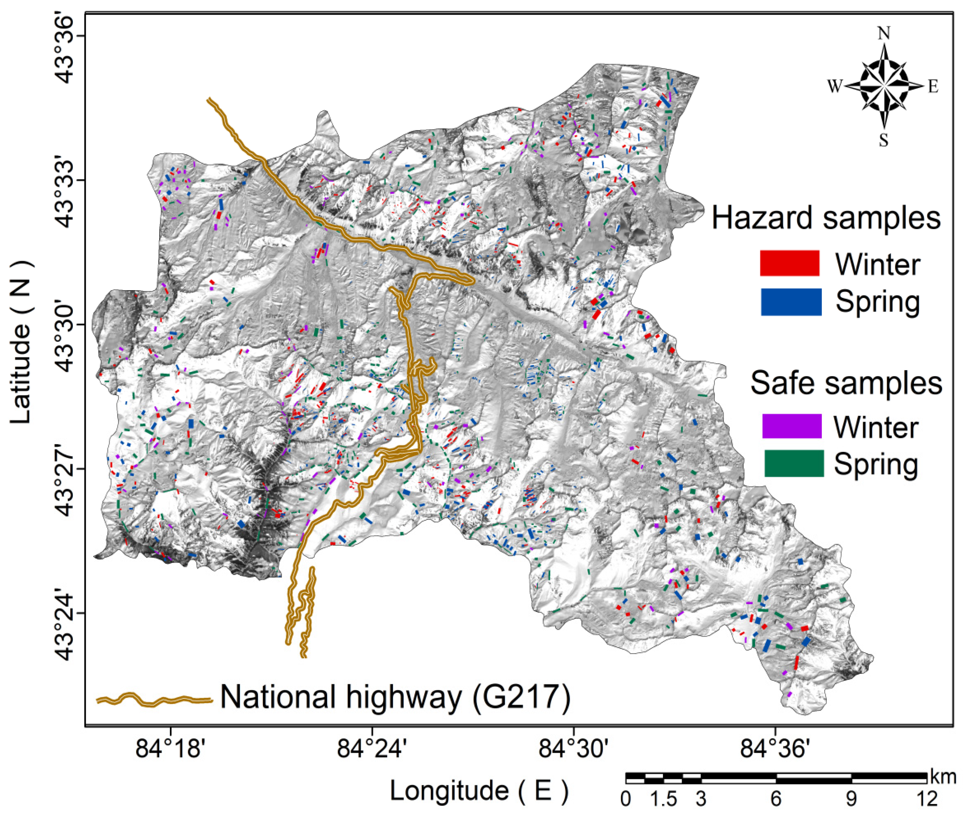
- Build a database of safety and hazard samples in winter and spring based on the high-precision and large-capacity avalanche inventory;
- Optimise the evaluation factors with multicollinearity and relief-F and clarify the key elements that affect avalanche hazard in these two seasons;
- Predict the susceptibility to avalanches in winter and spring using the SVM model, RF model and KNN model, and interpret the distribution and seasonal characteristics;
- Verify and compare the performance of the optimised multi-source heterogeneous factor models.
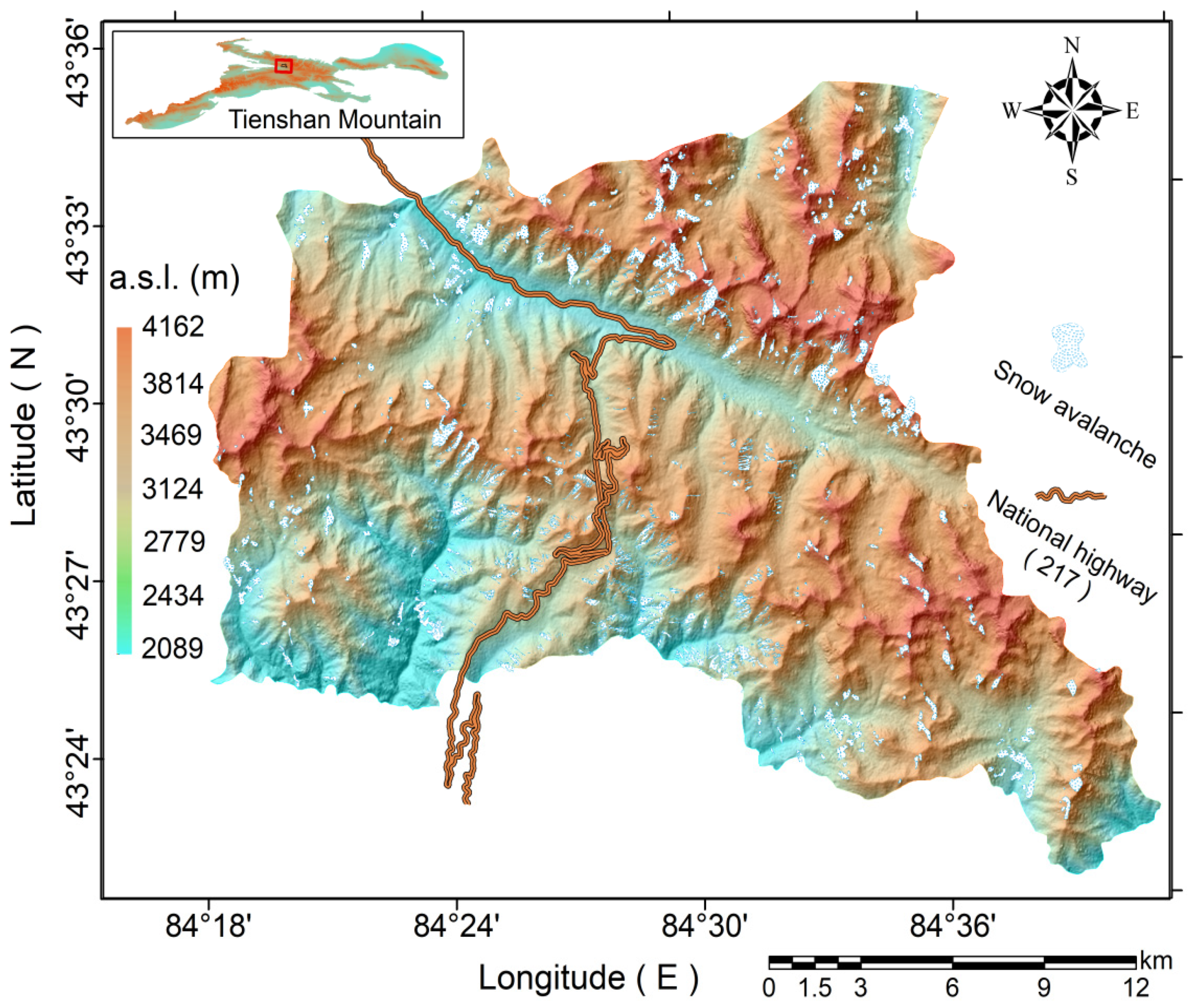
2. Study Area
3. Data Collecting and Processing
3.1. Avalanche Inventory Data
3.1.1. Satellite Observation
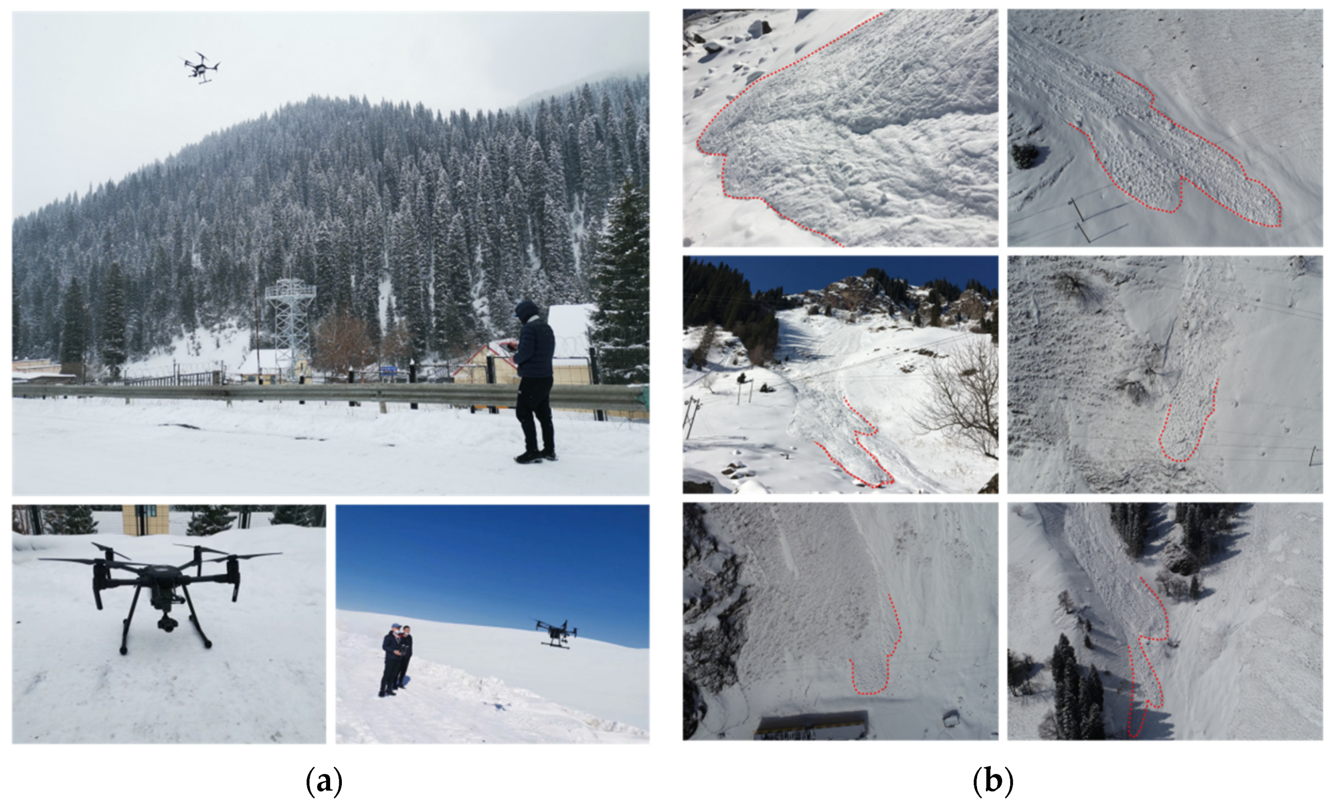
3.1.2. Avalanche Inventory Obtained by UAV Photography
3.1.3. Avalanche Inventory from Field Investigation
3.2. Causative Factors
3.2.1. Topographic Factors
Elevation
Slope
Aspect
Plane and Profile Curvature
TRI
TPI
VRM
TST
RDLS
DTS
TWI
DTR
Solar Radiation
3.2.2. Meteorological Factors
Temperature
Wind Speed
3.2.3. LUCC
3.2.4. Earthquake Hazard Distributions
3.2.5. Snow-Related Variables
Snow Depth
NDSI
3.3. Methodology
3.3.1. Multicollinearity
3.3.2. Feature Selection
3.3.3. Mann–Whitney U Test
3.3.4. SVM
3.3.5. RF
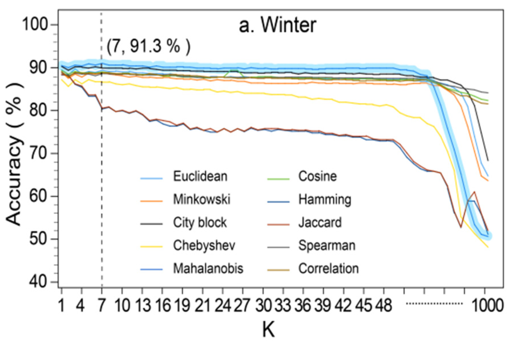
3.3.6. KNN
3.4. Performance Verification of the Model
3.4.1. ROC
3.4.2. Statistical Indicators
3.5. Experimental Design
- Collect complete and accurate avalanche inventory in Taldasha and establish a sample database through the integrated avalanche survey network of “space–air–ground”. Establish a hazard driving-factor database related to topography, meteorology, surface cover, crustal dynamics and snow conditions according to the local avalanche disaster-pregnant environment.
- Optimise the introduced drivers, including multicollinearity analysis and relief-F, and use the Mann–Whitney U test to verify the purity of the safe samples and hazard samples. Establish training samples and testing samples for spring and winter, respectively, on the basis of the above optimisation of the causative factors.
- Apply SVM, RF and KNN algorithms, respectively, to learn the samples. Build models with appropriate accuracy, and evaluate the avalanche hazard of Taldasha in winter and spring.
- Evaluate and compare the performance of the models.
4. Results
4.1. Avalanche Susceptibility Modeling
4.1.1. Multicollinearity Analysis
4.1.2. Elimination of the Less Important Causative Factors
4.1.3. Difference between Hazard Samples and Safety Samples
4.2. Avalanche Susceptibility Cartographic Representation
4.2.1. Parameterisation Scheme of Avalanche hazard Assessment Model
4.2.2. Spatial Characteristics of Avalanche Hazard
4.2.3. Seasonal Characteristics of Avalanche hazard
4.3. Model Performance Verification and Comparison
4.3.1. Using ROC
4.3.2. Using Accuracy Statistics
5. Discussion
5.1. Model Performance
5.1.1. Influence of Optimised Explanatory Variables on Model Accuracy
5.1.2. Advantages of the Model Framework
5.2. Limitations
6. Conclusions and Future Development
Author Contributions
Funding
Institutional Review Board Statement
Informed Consent Statement
Data Availability Statement
Acknowledgments
Conflicts of Interest
References
- Liu, Y.; Chen, X.; Qiu, Y.; Hao, J.; Yang, J.; Li, L. Mapping snow avalanche debris by object-based classification in moutainous regions from Sentinel-1 images and causative indices. Catena 2021, 206, 105559. [Google Scholar] [CrossRef]
- D’Aubeterre, G.; Favillier, A.; Mainieri, R.; Lopez, J.; Eckert, N.; Saulnier, M.; Peiry, J.; Stoffel, M.; Corona, C. Tree-ring reconstruction of snow avalanche activity: Does avalanche path selection matter? Sci. Total Environ. 2019, 684, 496–508. [Google Scholar] [CrossRef]
- Kumar, S.; Srivastava, P.K.; Snehmani; Bhatiya, S. Geospatial probabilistic modelling for release area mapping of snow avalanches. Cold Reg. Sci. Technol. 2019, 165, 102813. [Google Scholar] [CrossRef]
- Peitzsch, E.H.; Hendrikx, J.; Fagre, D.B. Terrain parameters of glide snow avalanches and a simple spatial glide snow avalanche model. Cold Reg. Sci. Technol. 2015, 120, 237–250. [Google Scholar] [CrossRef]
- Fischer, J.T. A novel approach to evaluate and compare computational snow avalanche simulation. Nat. Hazards Earth Syst. Sci. 2013, 13, 1655–1667. [Google Scholar] [CrossRef]
- Yariyan, P.; Avand, M.; Abbaspour, R.A.; Karami, M.; Tiefenbacher, J.P. GIS-based spatial modeling of snow avalanches using four novel ensemble models. Sci. Total Environ. 2020, 745, 141008. [Google Scholar] [CrossRef] [PubMed]
- Gądek, B.; Kaczka, R.J.; Rączkowska, Z.; Rojan, E.; Casteller, A.; Bebi, P. Snow avalanche activity in Żleb Żandarmerii in a time of climate change (Tatra Mts. Poland). Catena 2017, 158, 201–212. [Google Scholar] [CrossRef]
- Haraldsdóttir, S.H.; Ólafsson, H.; Durand, Y.; Giraud, G.; Mérindol, L. A system for prediction of avalanche hazard in the windy climate of Iceland. Ann. Glaciol. 2004, 38, 319–324. [Google Scholar] [CrossRef][Green Version]
- Engeset, R.V.; Pfuhl, G.; Landr, M.; Mannberg, A.; Hetland, A. Communicating public avalanche warnings-what works? Nat. Hazards Earth Syst. Sci. 2018, 18, 2537–2559. [Google Scholar] [CrossRef]
- Gruber, U.; Bartelt, P. Snow avalanche hazard modelling of large areas using shallow water numerical methods and GIS. Environ. Model. Softw. 2007, 22, 1472–1481. [Google Scholar] [CrossRef]
- Prabhjot, K.; Jagdish, C.J.; Preeti, A. A multi-model decision support system (MM-DSS) for avalanche hazard prediction over North-West Himalaya. Nat. Hazards 2021, 110, 563–585. [Google Scholar] [CrossRef]
- Barbara, M. An ArcGIS Geo-Morphological Approach for Snow Avalanche Zoning and hazard Estimation in the Province of Bergamo. J. Geogr. Inf. Syst. 2017, 9, 83–97. [Google Scholar] [CrossRef][Green Version]
- Aydin, A.; Eker, R. GIS-based snow avalanche hazard mapping: Bayburt-Așağı Dere catchment case. J. Environ. Biol. 2017, 38, 937–943. [Google Scholar] [CrossRef]
- Yariyan, P.; Omidvar, E.; Karami, M.; Cerdà, a.; Pham, Q.B.; Tiefenbacher, J.P. Evaluating novel hybrid models based on GIS for snow avalanche susceptibility mapping: A comparative study. Cold Reg. Sci. Technol. 2022, 194, 103453. [Google Scholar] [CrossRef]
- Parshad, R.; Srivastva, P.K.; Snehmani; Ganguly, S.; Kumar, S.; Ganju, A. Snow Avalanche Susceptibility Mapping using Remote Sensing and GIS in Nubra-Shyok Basin, Himalaya, India. Indian J. Sci. Technol. 2017, 10, 1–12. [Google Scholar] [CrossRef]
- Reichstein, M.; Camps-Valls, G.; Stevens, B.; Jung, M.; Denzler, J.; Carvalhais, N.; Prabhat. Deep learning and process understanding for data-driven Earth system science. Nature 2019, 566, 195–204. [Google Scholar] [CrossRef]
- Gall, J.; Yao, A.; Razavi, N.; Gool, L.V.; Lempitsky, V. Hough Forests for Object Detection, Tracking, and Action Recognition. IEEE Trans. Pattern Anal. Mach. Intell. 2011, 33, 2188–2202. [Google Scholar] [CrossRef]
- Vincent, C.; Soeren, P.; Reza, M.; Anelia, A. Depth Prediction Without the Sensors: Leveraging Structure for Unsupervised Learning from Monocular Videos. Proc. AAAI Conf. Artif. Intell. 2019, 33, 8001–8008. [Google Scholar] [CrossRef]
- Orazbayev, B.; Fleury, R. Far-field subwavelength acoustic imaging by deep learning. Phys. Rev. X 2020, 10, 031029. [Google Scholar] [CrossRef]
- Xiong, W.; Droppo, J.; Huang, X.; Seide, F.; Seltzer, M.; Stolcke, A.; Yu, D.; Zweig, G. Achieving Human Parity in Conversational Speech Recognition. IEEE/ACM Trans. Audio Speech Lang. Process. 2016, 1610, 05256. [Google Scholar] [CrossRef]
- Zacharaki, E.I.; Wang, S.; Chawla, S.; Yoo, D.S.; Wolf, R.; Melhem, E.R.; Davatzikos, C. Classification of brain tumor type and grade using MRI texture and shape in a machine learning scheme. Magn. Reson. Med. Off. J. Int. Soc. Magn. Reson. Med. 2009, 62, 1609–1618. [Google Scholar] [CrossRef] [PubMed]
- Yariyan, P.; Omidvar, E.; Minaei, F.; Abbaspour, R.A.; Tiefenbacher, J.P. An optimization on machine learning algorithms for mapping snow avalanche susceptibility. Nat. Hazards 2021, 108, 1–36. [Google Scholar] [CrossRef]
- Gassner, M.; Brabec, B. Nearest neighbour models for local and regional avalanche forecasting. Nat. Hazards Earth Syst. Sci. 2002, 2, 247–253. [Google Scholar] [CrossRef]
- Gauthier, F.; Germain, D.; Hétu, B. Logistic models as a forecasting tool for snow avalanches in a cold maritime climate: Northern Gaspésie, Québec, Canada. Nat. Hazards 2017, 89, 201–232. [Google Scholar] [CrossRef]
- Pozdnoukhov, A.; Matasci, G.; Kanevski, M.; Purves, R.S. Spatio-temporal avalanche forecasting with Support Vector Machines. Nat. Hazards Earth Syst. Sci. 2011, 11, 367–382. [Google Scholar] [CrossRef]
- Tiwari, A.; Arun, G.; Vishwakarma, B.D. Parameter importance assessment improves efficacy of machine learning methods for predicting snow avalanche sites in Leh-Manali Highway, India. Sci. Total Environ. 2021, 794, 148738. [Google Scholar] [CrossRef]
- Choubin, B.; Borji, M.; Mosavi, A.; Sajedi-Hosseini, F.; Singh, V.P.; Shamshirband, S. Snow avalanche hazard prediction using machine learning methods. J. Hydrol. 2019, 577, 123929. [Google Scholar] [CrossRef]
- Chawla, M.; Singh, A. Data efficient Random Forest model for avalanche forecasting. Nat. Hazards Earth Syst. Sci. 2019, 379, 1–33. [Google Scholar] [CrossRef]
- Rahmati, O.; Ghorbanzadeh, O.; Teimurian, T.; Mohammadi, F.; Tiefenbacher, J.P.; Falah, F.; Pirasteh, S.; Thi Ngo, P.T.; Bui, D.T. Spatial Modeling of Snow Avalanche Using Machine Learning Models and Geo-Environmental Factors: Comparison of Effectiveness in Two Mountain Regions. Remote Sens. 2019, 11, 2995. [Google Scholar] [CrossRef]
- Yousefi, S.; Pourghasemi, H.R.; Emami, S.N.; Pouyan, S.; Eskandari, S.; Tiefenbacher, J.P. A machine learning framework for multi-hazards modeling and mapping in a mountainous area. Sci. Rep. 2020, 10, 12144. [Google Scholar] [CrossRef]
- Rahmati, O.; Yousefi, S.; Kalantari, Z.; Uuemaa, E.; Teimurian, T.; Keesstra, S.; Pham, T.D.; Bui, D.T. Multi-hazard exposure mapping using machine learning techniques: A case study from Iran. Remote Sens. 2019, 11, 1943. [Google Scholar] [CrossRef]
- Choubin, B.; Borji, M.; Hosseini, F.S.; Mosavi, A.; Dineva, A.A. Mass wasting susceptibility assessment of snow avalanches using machine learning models. Sci. Rep. 2020, 10, 18363. [Google Scholar] [CrossRef] [PubMed]
- Zhang, S.; Li, X.; Zong, M.; Zhu, X.F.; Cheng, D. Learning k for kNN classification. ACM Trans. Intell. Syst. Technol. 2017, 8, 1–19. [Google Scholar] [CrossRef]
- Bühler, Y.; Hafner, E.D.; Zweifel, B.; Zesiger, M.; Heisig, H. Where are the avalanches? Rapid mapping of a large snow avalanche period with optical satellites. Cryosphere Discuss. 2019, 119, 1–21. [Google Scholar] [CrossRef]
- Korzeniowska, K.; Bühler, Y.; Marty, M.; Korup, O. Regional snow-avalanche detection using object-based image analysis of near-infrared aerial imagery. Nat. Hazards Earth Syst. Sci. 2017, 17, 1823–1836. [Google Scholar] [CrossRef]
- Gong, P.; Chen, B.; Li, X.C.; Liu, H.; Wang, J.; Bai, Y.Q.; Chen, J.M.; Chen, X.; Fang, L.; Feng, S.L.; et al. Mapping essential urban land use categories in China (EULUC-China): Preliminary results for 2018—Science Direct. Sci. Bull. 2020, 65, 182–187. [Google Scholar] [CrossRef]
- Viviana, M.; Christian, M. Chapter fifteen: Snow avalanche. In Extreme Hydroclimatic Events and Multivariate Hazards in a Changing Environment; Viviana, M., Christian, M., Eds.; Elsevier: Amsterdam, The Netherlands, 2019; pp. 369–389. [Google Scholar] [CrossRef]
- Milena, R.; Piotr, M.; Aleksandra, M. Topographic Wetness Index and Terrain Ruggedness Index in geomorphic characterisation of landslide terrains, on examples from the Sudetes, SW Poland. Z. Fur Geomorphol. Suppl. 2017, 61, 61–80. [Google Scholar] [CrossRef]
- You, Z.; Feng, Z.M.; Yang, Y.Z. Relief Degree of Land Surface Dataset of China (1 km). J. Glob. Change Data Discov. 2018, 2, 151–155. [Google Scholar] [CrossRef]
- Zheng, W.; Ning, H. The effect of mountain wind on the falling snow deposition. J. Phys. Conf. Ser. 2017, 822, 012050. [Google Scholar] [CrossRef]
- Mosavi, A.; Shirzadi, A.; Choubin, B.; Taromideh, F.; Hosseini, F.S.; Borji, M.; Shahabi, H.; Salvati, A.; Dineva, A.A. Towards an ensemble machine learning model of random subspace based functional tree classifier for snow avalanche susceptibility mapping. IEEE Access 2020, 8, 145968–145983. [Google Scholar] [CrossRef]
- Costache, R.; Hong, H.Y.; Pham, Q.B. Comparative assessment of the flash-flood potential within small mountain catchments using bivariate statistics and their novel hybrid integration with machine learning models. Sci. Total Environ. 2020, 711, 134514. [Google Scholar] [CrossRef] [PubMed]
- Urbanowicz, R.J.; Meeker, M.; Cava, W.L.; Olson, R.S.; Moore, J.H. Relief-Based Feature Selection: Introduction and Review. J. Biomed. Inform. 2018, 85, 189–203. [Google Scholar] [CrossRef] [PubMed]
- MacFarland, T.W.; Yates, J.M. Introduction to Nonparametric Statistics for the Biological Sciences Using R; Springer: Cham, Switzerland, 2016; pp. 103–132. [Google Scholar]
- Kavzoglu, T.; Colkesen, I.; Sahin, E.K. Machine learning techniques in landslide susceptibility mapping: A survey and a case study. In Landslides: Theory, Practice and Modeling; Pradhan, S.P., Vishal, V., Singh, T.N., Eds.; Springer: Cham, Switzerland, 2019; Volume 50, pp. 283–301. [Google Scholar] [CrossRef]
- Tharwat, A. Parameter investigation of support vector machine classifier with kernel functions. Knowl. Inf. Syst. 2019, 61, 1269–1302. [Google Scholar] [CrossRef]
- Wang, H.J.; Zhang, L.M.; Yin, K.S.; Luo, H.Y.; Li, J.H. Landslide identification using machine learning. Geosci. Front. 2021, 12, 351–364. [Google Scholar] [CrossRef]
- Merghadi, A.; Yunus, A.P.; Dou, J.; Whiteley, J.; Thaipham, B.; Bui, D.T.; Avtar, R.; Abderrahrmane, B. Machine learning methods for landslide susceptibility studies: A comparative overview of algorithm performance. Earth-Sci. Rev. 2020, 207, 103225. [Google Scholar] [CrossRef]
- Tewari, S.; Dwivedi, U.D. A comparative study of heterogeneous ensemble methods for the identification of geological lithofacies. J. Pet. Explor. Prod. Technol. 2020, 10, 1849–1868. [Google Scholar] [CrossRef]
- Ozigis, M.S.; Kaduk, J.D.; Jarvis, C.H.; Bispo, P.C.; Balzter, H. Detection of oil pollution impacts on vegetation using multifrequency SAR, multispectral images with fuzzy forest and random forest methods. Environ. Pollut. 2020, 256, 113360. [Google Scholar] [CrossRef]
- Statham, G.; Haegeli, P.; Greene, E.; Birkeland, K.; Israelson, C.; Tremper, B.; Stethem, C.; McMahon, B.; White, B.; Kelly, J. A conceptual model of avalanche hazard. Nat. Hazards 2018, 90, 663–691. [Google Scholar] [CrossRef]
- Chen, J.; Yang, S.T.; Li, H.W.; Zhang, B.; Lv, J.R. Research on Geographical Environment Unit Division Based on the Method of Natural Breaks (Jenks). ISPRS-Int. Arch. Photogramm. Remote Sens. Spat. Inf. Sci. 2013, XL-4/W3, 47–50. [Google Scholar] [CrossRef]
- Puzrin, A.M.; Faug, T.; Einav, I. The mechanism of delayed release in earthquake-induced avalanches. Proc. R. Soc. A Math. Phys. Eng. Sci. 2019, 475, 20190092. [Google Scholar] [CrossRef] [PubMed]
- Helbig, N.; Van, H.A.; Jonas, T. Forecasting wet-snow avalanche probability in mountainous terrain. Cold Reg. Sci. Technol. 2015, 120, 219–226. [Google Scholar] [CrossRef]
- Schweizer, J.; Mitterer, C.; Stoffel, L. On forecasting large and infrequent snow avalanches. Cold Reg. Sci. Technol. 2009, 59, 234–241. [Google Scholar] [CrossRef]
- Sherif, A.A.E.; Sk, A.A.; Quoc, B.P. Spatial modeling and susceptibility zonation of landslides using random forest, naïve bayes and K-nearest neighbor in a complicated terrain. Earth Sci. Inform. 2021, 14, 1227–1243. [Google Scholar] [CrossRef]
- Yasin, W.R.; Md, B.H.; Joynal, A. Landslide Susceptibility Mapping in Three Upazilas of Rangamati Hill District Bangladesh: Application and Comparison of GIS-based Machine Learning Methods. Geocarto Int. 2020, 35, 1–27. [Google Scholar] [CrossRef]
- Christen, M.; Kowalski, J.; Bartelt, P. RAMMS: Numerical simulation of dense snow avalanches in three dimensional terrain. Cold Reg. Sci. Technol. 2010, 63, 1–14. [Google Scholar] [CrossRef]
- Fischer, J.T.; Fromm, R.; Gauer, P.; Sovilla, B. Evaluation of probabilistic snow avalanche simulation ensembles with Doppler radar observations. Cold Reg. Sci. Technol. 2014, 97, 151–158. [Google Scholar] [CrossRef]


| Physical Model | |
| Advantages | Can precisely describe the snow instability process and avalanche dynamics on a single predefined slope. |
| Disadvantages | Higher reliance on special input data. Drive data is difficult to obtain. Limited scale of assessment. |
| Data-Driven | |
| Advantages | Easy to implement. Satisfying visualisation. |
| Disadvantages | The evaluation results have certain uncertainty and human subjectivity. The variable selection process has a certain one-sidedness and fuzziness. |
| Machine Learning | |
| Advantages | The evaluation results are objective and accurate. The evaluation model can be replicated and extended. Avalanche hazard can be assessed on a large scale. |
| Disadvantages | High requirements for the quality and quantity of sample data. |
| Field Observation Assessment | |
| Advantages | Daily evaluation possible. |
| Disadvantages | Evaluation results vary and are subjective due to the specialisation of the observers. Avalanches occur suddenly, resulting in very limited opportunities to prepare and issue alerts. The scope of the assessment is limited by the natural conditions and the accessibility of the road network. |
| Parameter Statistics | Details | ||||
|---|---|---|---|---|---|
| Bands | Multispectral | Panchromatic | |||
| Red | Green | Blue | Near Infrared | ||
| Spectral range (mm) | 450–520 | 520–590 | 630–690 | 770–890 | 450–890 |
| Spatial resolution | 2.0 m | 50 cm | |||
| Revisit period | 1 d | ||||
| Ground sampling interval | 2.0 m | ||||
| Cloud cover | 0.5–2.7% | ||||
| Variables | Winter | Spring | Control Group | |||
|---|---|---|---|---|---|---|
| TOL | VIF | TOL | VIF | TOL | VIF | |
| Elevation | 0.751 | 1.332 | 0.713 | 1.403 | 0.675 | 1.480 |
| Slope | 0.921 | 1.086 | 0.930 | 1.076 | 0.734 | 1.447 |
| Aspect | 0.661 | 1.512 | 0.853 | 1.172 | 0.857 | 1.167 |
| Plane curvature | 0.494 | 2.025 | 0.676 | 1.479 | 0.613 | 1.631 |
| Profile curvature | 0.579 | 1.726 | 0.546 | 1.832 | 0.588 | 1.701 |
| TRI | 0.247 | 4.048 | 0.386 | 2.591 | 0.736 | 1.142 |
| TPI | 0.383 | 2.613 | 0.395 | 2.534 | 0.409 | 2.445 |
| VRM | 0.706 | 1.416 | 0.691 | 1.447 | 0.718 | 1.393 |
| TST | 0.594 | 1.684 | 0.610 | 1.640 | 0.642 | 1.557 |
| RDLS | 0.274 | 3.653 | 0.548 | 1.823 | 0.665 | 1.504 |
| DTS | 0.921 | 1.085 | 0.853 | 1.173 | 0.973 | 1.028 |
| TWI | 0.351 | 2.851 | 0.312 | 3.201 | 0.317 | 3.152 |
| DTR | 0.761 | 1.315 | 0.551 | 1.815 | 0.895 | 1.118 |
| Solar radiation | 0.682 | 1.466 | 0.586 | 1.708 | 0.631 | 1.586 |
| Temperature | 0.637 | 1.570 | 0.184 | 5.424 | 0.501 | 1.937 |
| Wind speed | 0.452 | 2.214 | 0.204 | 4.902 | 0.147 | 6.808 |
| LUCC | 0.959 | 1.042 | 0.947 | 1.056 | 0.913 | 1.095 |
| Earthquake hazard distribution | 0.744 | 1.345 | 0.713 | 1.403 | 0.817 | 1.223 |
| Snow depth | 0.518 | 1.932 | 0.673 | 1.486 | 0.407 | 2.457 |
| Winter | Spring | Control Group | |||
|---|---|---|---|---|---|
| Causative Factors | Weight | Causative Factors | Weight | Causative Factors | Weight |
| RDLS | 14.18% | Snow depth | 17.33% | DTS | 10.11% |
| Slope | 10.72% | DTR | 13.95% | DTR | 10.11% |
| TST | 9.24% | Temperature | 7.84% | Aspect | 9.72% |
| Elevation | 9.07% | Elevation | 7.02% | Slope | 9.19% |
| DTS | 8.76% | LUCC | 6.21% | Solar radiance | 8.82% |
| TPI | 7.58% | TST | 5.69% | RDLS | 8.77% |
| DTR | 6.85% | Slope | 5.65% | Elevation | 8.47% |
| Snow depth | 5.97% | TPI | 5.22% | Profile curvature | 6.97% |
| Temperature | 5.74% | TWI | 4.69% | TPI | 5.82% |
| TRI | 4.87% | RDLS | 4.61% | TWI | 5.72% |
| Aspect | 4.36% | VRM | 4.26% | TST | 4.85% |
| Solar radiance | 3.43% | Plane curvature | 4.06% | Temperature | 3.22% |
| VRM | 3.38% | Wind speed | 3.98% | LUCC | 2.33% |
| TWI | 1.82% | Earthquake hazard distribution | 3.71% | TRI | 2.26% |
| Wind speed | 1.77% | Profile curvature | 2.64% | Snow depth | 1.67% |
| Profile curvature | 1.03% | Aspect | 2.07% | Earthquake hazard distribution | 1.14% |
| LUCC | 0.64% | DTS | 0.59% | Wind speed | 0.69% |
| Earthquake hazard distribution | 0.62% | Solar radiance | 0.48% | Plane curvature | 0.19% |
| Plane curvature | 0.00% | TRI | 0.00% | VRM | 0.00% |
| Variables | Spring | Winter | Control Group | |||
|---|---|---|---|---|---|---|
| U-Test | Sig. | U-Test | Sig. | U-Test | Sig. | |
| Elevation | 835,967.5 | 0.002 | 449,809.0 | 0.000 | 4,835,510.5 | 0.000 |
| Slope | 1,511,322.5 | 0.000 | 1,134,259.5 | 0.000 | 10,501,820.5 | 0.000 |
| Aspect | 767,895.0 | 0.029 | 625,725.5 | 0.030 | 5,792,301.5 | 0.000 |
| Plane curvature | 2,640.0 | 0.000 | 1,163,187.0 | 0.000 | 4,877,144.5 | 0.000 |
| Profile curvature | 1,487,844.0 | 0.000 | 1,007,208.0 | 0.000 | 6,170,964.5 | 0.000 |
| TRI | 1,549,211.0 | 0.000 | 1,163,790.0 | 0.000 | 10,470,029.0 | 0.000 |
| TPI | 15,550,256.0 | 0.000 | 1,154,167.0 | 0.000 | 3,861,983.0 | 0.000 |
| VRM | 0.0 | 0.000 | 1,163,790.0 | 0.000 | 4,625,425.5 | 0.000 |
| TST | 1,554,297.0 | 0.000 | 1,162,073.0 | 0.000 | 6,165,772.5 | 0.000 |
| RDLS | 1,506,172.0 | 0.000 | 235,121.0 | 0.000 | 9,838,493.5 | 0.000 |
| DTS | 903,403.5 | 0.000 | 740,014.5 | 0.000 | 6,824,133.0 | 0.000 |
| TWI | 1,557,600.0 | 0.000 | 1,163,731.0 | 0.000 | 4,790,261.0 | 0.000 |
| DTR | 1,036,784.5 | 0.000 | 757,006.5 | 0.000 | 5,488,534.5 | 0.024 |
| Solar radiation | 977,256.5 | 0.000 | 500,320.5 | 0.000 | 3,704,101.0 | 0.000 |
| Temperature | 1,169,421.0 | 0.000 | 1,127,098.0 | 0.000 | 5,724,934.0 | 0.000 |
| Wind speed | 274,446.0 | 0.000 | 0.0 | 0.000 | 5,133,122.5 | 0.001 |
| LUCC | 899,652.0 | 0.000 | 384,258.0 | 0.000 | 4,280,161.0 | 0.000 |
| Earthquake hazard distribution | 865,046.0 | 0.000 | 633,830.5 | 0.000 | 5,453,588.5 | 0.016 |
| Snow depth | 1,281,572.0 | 0.000 | 0.0 | 0.000 | 5,678,461.0 | 0.000 |
| Seasons | Kernel | C | g | Number of Support Vectors | AUC |
|---|---|---|---|---|---|
| Winter | Linear | 1 | / | 331 | 0.897 |
| Polynomial | 1 | 0.5 | 210 | 0.886 | |
| RBF | 1 | 0.5 | 247 | 0.992 | |
| Sigmoid | 1 | 0.5 | 780 | 0.846 | |
| Spring | Linear | 1 | / | 482 | 0.801 |
| Polynomial | 1 | 0.5 | 325 | 0.931 | |
| RBF | 1 | 0.5 | 564 | 0.994 | |
| Sigmoid | 1 | 0.5 | 747 | 0.928 | |
| Control group | Linear | 1 | / | 486 | 0.885 |
| Polynomial | 1 | 0.5 | 291 | 0.898 | |
| RBF | 1 | 0.5 | 897 | 0.995 | |
| Sigmoid | 1 | 0.5 | 722 | 0.880 |
| Cases | Classifier | Statistics | ||||
|---|---|---|---|---|---|---|
| MCC | OA | FOM | POFD | FB | ||
| Winter | SVM | 0.815 | 0.892 | 0.131 | 0.086 | 0.892 |
| RF | 0.965 | 0.935 | 0.111 | 0.014 | 0.652 | |
| KNN | 0.829 | 0.772 | 0.092 | 0.292 | 1.011 | |
| Spring | SVM | 0.760 | 0.757 | 0.270 | 0.188 | 0.600 |
| RF | 0.905 | 0.985 | 0.003 | 0.063 | 0.989 | |
| KNN | 0.770 | 0.796 | 0.264 | 0.120 | 1.218 | |
| Control group | SVM | 0.552 | 0.688 | 0.655 | 0.460 | 1.160 |
| RF | 0.687 | 0.730 | 0.219 | 0.297 | 0.754 | |
| KNN | 0.423 | 0.612 | 0.393 | 0.357 | 1.601 | |
| SVM | ||||||
|---|---|---|---|---|---|---|
| Seasons | Types of Factors Applied One by One | Accuracy Statistics | ||||
| MCC | OA | FOM | POFD | FB | ||
| Winter | Topographic | 0.109 | 0.542 | 0.562 | 0.450 | 1.789 |
| Atmosphere | 0.393 | 0.561 | 0.500 | 0.300 | 1.421 | |
| LUCC | 0.489 | 0.578 | 0.472 | 0.272 | 1.101 | |
| Crustal movement | 0.528 | 0.618 | 0.400 | 0.200 | 0.774 | |
| Spring | Topographic | 0.306 | 0.501 | 0.362 | 0.470 | 0.675 |
| Atmosphere | 0.328 | 0.542 | 0.262 | 0.376 | 0.626 | |
| LUCC | 1.011 | 0.673 | 0.206 | 0.352 | 0.513 | |
| Crustal movement | 0.541 | 0.779 | 0.171 | 0.271 | 0.648 | |
| RF | ||||||
|---|---|---|---|---|---|---|
| Seasons | Types of Factors Applied One by One | Accuracy Statistics | ||||
| MCC | OA | FOM | POFD | FB | ||
| Winter | Topographic | 0.595 | 0545 | 0.333 | 0.530 | 1.543 |
| Atmosphere | 0.679 | 0.632 | 0.258 | 0.500 | 1.746 | |
| LUCC | 0.719 | 0.770 | 0.200 | 0.327 | 1.603 | |
| Crustal movement | 0.799 | 0.848 | 0.163 | 0.258 | 0.500 | |
| Spring | Topographic | 0.695 | 0.645 | 0.433 | 0.534 | 0.543 |
| Atmosphere | 0.705 | 0.705 | 0.334 | 0.495 | 0.543 | |
| LUCC | 0.749 | 0.745 | 0.295 | 0.344 | 0.415 | |
| Crustal movement | 0.781 | 0.841 | 0.264 | 0.278 | 0.641 | |
| KNN | ||||||
|---|---|---|---|---|---|---|
| Seasons | Types of Factors Applied One by One | Accuracy Statistics | ||||
| MCC | OA | FOM | POFD | FB | ||
| Winter | Topographic | −0.219 | 0.410 | 0.424 | 0.652 | 1.603 |
| Atmosphere | 2.062 | 0.421 | 0.394 | 0.424 | 1.553 | |
| LUCC | 1.145 | 0.550 | 0.336 | 0.336 | 1.433 | |
| Crustal movement | 0.249 | 0.611 | 0.336 | 0.297 | 1.285 | |
| Spring | Topographic | 1.719 | 0.352 | 0.424 | 0.652 | 1.653 |
| Atmosphere | 1.631 | 0.413 | 0.394 | 0.424 | 1.453 | |
| LUCC | 1.510 | 0.521 | 0.289 | 0.458 | 1.383 | |
| Crustal movement | −0.427 | 0.563 | 0.158 | 0.389 | 1.301 | |
Publisher’s Note: MDPI stays neutral with regard to jurisdictional claims in published maps and institutional affiliations. |
© 2022 by the authors. Licensee MDPI, Basel, Switzerland. This article is an open access article distributed under the terms and conditions of the Creative Commons Attribution (CC BY) license (https://creativecommons.org/licenses/by/4.0/).
Share and Cite
Yang, J.; He, Q.; Liu, Y. Winter–Spring Prediction of Snow Avalanche Susceptibility Using Optimisation Multi-Source Heterogeneous Factors in the Western Tianshan Mountains, China. Remote Sens. 2022, 14, 1340. https://doi.org/10.3390/rs14061340
Yang J, He Q, Liu Y. Winter–Spring Prediction of Snow Avalanche Susceptibility Using Optimisation Multi-Source Heterogeneous Factors in the Western Tianshan Mountains, China. Remote Sensing. 2022; 14(6):1340. https://doi.org/10.3390/rs14061340
Chicago/Turabian StyleYang, Jinming, Qing He, and Yang Liu. 2022. "Winter–Spring Prediction of Snow Avalanche Susceptibility Using Optimisation Multi-Source Heterogeneous Factors in the Western Tianshan Mountains, China" Remote Sensing 14, no. 6: 1340. https://doi.org/10.3390/rs14061340
APA StyleYang, J., He, Q., & Liu, Y. (2022). Winter–Spring Prediction of Snow Avalanche Susceptibility Using Optimisation Multi-Source Heterogeneous Factors in the Western Tianshan Mountains, China. Remote Sensing, 14(6), 1340. https://doi.org/10.3390/rs14061340