Abstract
In hyperspectral remote sensing, the clustering technique is an important issue of concern. Affinity propagation is a widely used clustering algorithm. However, the complex structure of the hyperspectral image (HSI) dataset presents challenge for the application of affinity propagation. In this paper, an improved version of affinity propagation based on complex wavelet structural similarity index and local outlier factor is proposed specifically for the HSI dataset. In the proposed algorithm, the complex wavelet structural similarity index is used to calculate the spatial similarity of HSI pixels. Meanwhile, the calculation strategy of the spatial similarity is simplified to reduce the computational complexity. The spatial similarity and the traditional spectral similarity of the HSI pixels jointly constitute the similarity matrix of affinity propagation. Furthermore, the local outlier factors are applied as weights to revise the original exemplar preferences of the affinity propagation. Finally, the modified similarity matrix and exemplar preferences are applied, and the clustering index is obtained by the traditional affinity propagation. Extensive experiments were conducted on three HSI datasets, and the results demonstrate that the proposed method can improve the performance of the traditional affinity propagation and provide competitive clustering results among the competitors.
1. Introduction
Hyperspectral image (HSI) has gradually become a powerful tool with its rich spectral and spatial information, which is widely used in environmental monitoring, fine agriculture, mineral exploration, military targets, and many other fields [1,2,3]. Though the potentialities of hyperspectral technology appear to be relatively wide, the analysis and treatment of these data remain insufficient [4]. Classification is an important manner in which to exploit HSI, which can be divided into supervised classification and unsupervised classification. Compared with the supervised classification, the unsupervised classification, also known as clustering, can automatically detect the distinct classes in an objective way without training samples. In fact, training samples are very difficult to access for some applications. As a result, it is meaningful to study the clustering technology.
Thus, in this paper, we mainly focused on the clustering approach for HSI partitioning. Generally speaking, clustering techniques can be mainly categorized into nine main types [5]: centroid-based clustering [6,7,8], density-based clustering [9,10,11], probability-based clustering [12,13,14,15], bionics-based clustering [16,17], intelligent computing-based clustering [18,19], graph-based clustering [20,21], subspace clustering [22,23,24,25], deep learning-based clustering [26,27,28], and hybrid mechanism-based clustering [29,30]. Affinity propagation (AP) [31] is a centroid-based clustering method that identifies a set of data points that best represent the dataset and assigns each data point to a single exemplar. Compared with classical centroid-based clustering, AP is insensitive to the initial centers and outliers. Therefore, it is widely used in face recognition [32], HSI classification [33], fault detection [34], and many other fields [35,36,37]. At the same time, many scholars have carried out in-depth studies of AP and put forward improved versions. The measuring of the similarity is a topic that has received a lot of attention. Wan, X. J. et al. [38] used dynamic time warping to measure the similarity between the original time series data and obtained the similarity between the corresponding components, which was applied to cluster the multivariate time series data with AP. Wang, L. M. et al. [39] proposed a novel structural similarity to solve the unsatisfactory clustering impact of AP when dealing with complex structural datasets. Zhang, W. et al. [40] applied soft scale invariant feature transform to adopt the similarity between any pair of images to clustering the images by AP. Qin, Y. et al. [41] integrated the spatial-spectral information of HSI samples into non-negative matrix factorization for affinity matrix learning of HSI clustering. Fan, L. et al. [42] proposed a local density adaptive affinity matrix, which embeds both spectral and spatial information and uses it for HSI clustering. We can see that these algorithms use tailored similarity for datasets to increase the performance of the clustering methods. Meanwhile, many studies have aimed at optimizing the exemplar preference of AP. Chen, D. W. et al. [43] defined a novel stability measure for AP to automatically select the appropriate exemplar preferences. Gan, G. J. and M. K. P. Ng [44] proposed a subspace clustering algorithm by introducing attribute weights in the AP. The new step could iteratively update the exemplar preferences to identify the subspaces in which clusters are embedded. Li, P. et al. [45] proposed a modified AP named as adjustable preference affinity propagation, which initials the value of preferences according to the data distribution. In addition, the convergence speed [46] and the calculation scale [4] are also mentioned in the literature.
However, the application of AP for HSI analysis is still insufficient. The reasons are mainly twofold: (1) the complex spectral structure of the HSI dataset; and (2) the usage of the spatial information of the HSI dataset. As a result, it is meaningful to apply a spatial-spectral strategy to extract information from the HSI dataset, which can better express the similarity between samples. Moreover, it is also an interesting question to modify the value of the exemplar preference based on the characteristics of the HSI dataset.
The structural similarity (SSIM) index [47] was proposed as a promising metric of image, which accounts for spatial correlations. Aside from the mean intensity and contrast, the structural information of an image is described as those attributes that represent the structures of the objects in the visual scene. The complex wavelet SSIM index [48], also called CW-SSIM, is a type of SSIM in the spatial and complex wavelet domains. The structure information is represented by the spatial distribution of grayscale values as well as the magnitude and phase responses of the multidirectional Gabor filters. The CW-SSIM has been shown to be a useful measure in image quality assessment [49,50], feature extraction [51], and anomaly detection [52]. On the other hand, the local outlier factor (LOF) [53] was first used in the noisy detection in HSI analysis [54]. The calculation of LOF is related to a restricted local region around an object [55]. Yu, S. Q. et al. [56] proposed a low-rank representation in the field of hyperspectral anomaly detection, which facilitates the discrimination between the anomalous targets and background by utilizing a novel dictionary and an adaptive filter based on the local outlier factor. Few studies can be found that have applied CW-SSIM and LOF to express the similarity of samples in HSI datasets and generate the similarity matrix of AP. We applied the strategy of the CW-SSIM as well as the LOF to act on the traditional pixel-based similarity metric and the exemplar preference, respectively, and used them in AP for HSI clustering.
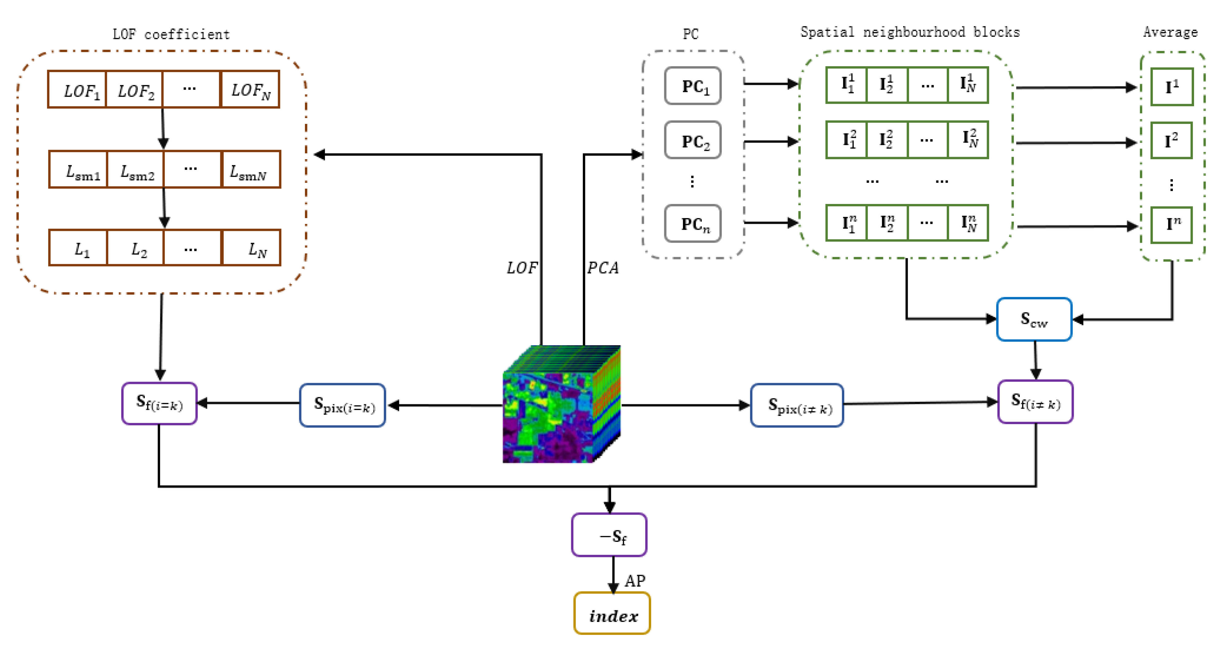
In this paper, an improved AP with CW-SSIM and LOF (CLAP) is presented based on the properties of hyperspectral data. The metrics of the similarity and the exemplar preference are both of concern in the proposed CLAP. Unlike the traditional approach that only calculates the pixel-based spectral similarity [57] to generate the similarity matrix of AP, the CLAP claims to combine the structure-based spatial similarity with pixel-based spectral similarity. In the proposed algorithm, the CW-SSIM is used to extract the structure-based spatial similarity of the HSI samples. To reduce the computational effort, we used principal component analysis (PCA) to reduce the sample size, and defined a novel strategy to reduce the computational complexity. Specifically, PCA was used to pre-process the hyperspectral data, and the dimensions of the highest explained principal components were reserved to extract the spatial information. We extracted the spatial neighborhood blocks of the samples on each principal component (PC) and recomposed new sample sets separately. After that, to reduce the computational complexity, the average of the samples for each principal component sample set was calculated, which was named Average, and the CW-SSIM was applied to calculate the similarity between samples and the corresponding Average. Then, the results were used to generate the spatial similarity matrix (). Finally, the final similarity matrix () was obtained by the pixel-based spectral similarity matrix () and the structure-based spatial similarity matrix (). Meanwhile, unlike the traditional definition of the consistent exemplar preferences that are directly based on the minimum (mean) value of the similarity, the CLAP uses the LOF to generate the weights to revise these consistent exemplar preferences. The key idea behind this is that the local neighborhood density of the cluster center should be uniform and smooth, according to the manifold assumption. Specifically, we first calculated the LOFs for all samples. Then, these LOFs were used to obtain the smoothness coefficients () by a self-defined formula, which represent the degree of the uniformity and smoothness of the local neighbourhood density of the samples on the spectral space. The LOF coefficients () were obtained using the smooth coefficients () and applied as weights to weight the original consistent preferences () to obtain the final exemplar preferences (). Finally, was used as the similarity matrix of AP and the clustering index of the samples were obtained by AP clustering. The flow chart of the proposed CLAP is shown in Figure 1. The novel contributions in the proposed method are as follows:
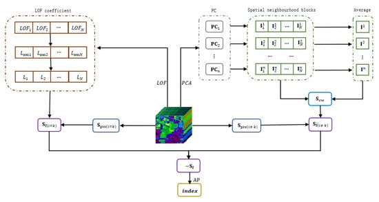
Figure 1.
The flow chart of the affinity propagation based on the structural similarity and local outlier factor.
- 1.
- New spatial-spectral similarity metrics for the hyperspectral dataset were defined and applied to AP clustering.
- 2.
- The CW-SSIM was used to measure the similarity of the HSI samples and a new computational strategy was defined to reduce the computational effort.
- 3.
- The LOF was used to define the degree of the uniformity and smoothness of the local neighborhood density of a sample and applied to revise the exemplar preference of AP.
In this study, we used three hyperspectral datasets as benchmarks to compare the proposed method to traditional clustering methods. Experiments showed that the proposed method outperformed the competition.
2. Method
2.1. Affinity Propagation
The AP is a clustering algorithm based on the exemplar method. It finds a set of data points to exemplify the data, and associates each data point with one exemplar. Specifically, given the samples , is the dimension, is the number of data points, the AP first computes a similarity matrix of all samples, which is defined as:
where is the element of the similarity matrix and is defined by the opposite of the squared Euclidean distance. is the diagonal element of the similarity matrix and is called the exemplar preference, which is set to the minimum value of the similarity matrix. It represents the prior suitability of a data point to be the exemplar, and controls the number of the clusters of AP. Then, the AP exchanges messages between data points, which are named responsibility and availability .
where and are the elements of and , and are initialized to 0. To avoid the oscillations, and are damped as:
where is the factor of damping, which satisfies , and is the number of the iteration. Finally, the exemplar vector can be obtained as:
The AP is converged if the iterative number exceeds the predetermined value or the exemplar vector remains unchanged for some constant iterations.
2.2. Complex Wavelet Structural Similarity
The CW-SSIM is a type of structural similarity index based on local phase measurements in the spatial and complex wavelet domain, which is designed to coincide with the human perceptual system and could provide a good approximation of perceptual image quality [48,51,58]. The CW-SSIM index is designed to separate the phase from luminance distortion measurements and simultaneously insensitive to luminance and contrast changes. Specifically, a complex version [59] of the steerable pyramid transform is first applied to decompose the compared two images [60]. The complex wavelet coefficients are expressed as and . The CW-SSIM index is defined as:
where is the complex conjugate of , and is a small positive stabilizing constant. The value of the index ranges from 0 to 1, where 1 implies no structural distortion.
2.3. Local Outlier Factor
The LOF is an outlier index that indicates the degree of the outlier-ness of a sample [53,55]. The LOF exploits the density information from the local neighborhood of each sample in the feature space. Specifically, given a dataset , for any positive integer , the k-distance of sample , denoted as , is defined as the distance between and so that:
- 1.
- For at least samples , it holds that , and
- 2.
- For at most objects , it holds that .
Next, given the k-distance of , the k-distance neighborhood of contains every object whose distance from is not greater than the k-distance, in other words
where the sample is called the k-nearest neighbor of and is designated as . Next, the reachability distance of sample with respect to sample is defined as:
Then, the local reachability density of is defined as:
where is the number of the k-nearest neighbors of . Finally, the local outlier factor of is defined as:
The value of the LOF index ranges from to , where is a positive real number. For most that are deeply inside the cluster, the LOF of is approximately equal to 1.
2.4. Affinity Propagation Based on Structural Similarity Index and Local Outlier Factor
From the description of the AP, we can see that the similarity matrix has a great influence on the algorithm. The element demonstrates the similarity of a pair of samples, and directly participates in the message being exchanged between samples. Both experience and experiments show that it can effectively affect the performance of AP by changing the measurement of the similarity matrix. The is referred to as “preference”, which can influence the number of identified exemplars. Additionally, the sample with a larger value of preference is more likely to be chosen as the exemplar. In fact, the number of identified exemplars is not only influenced by the values of the input preferences, but also emerges from the message-passing procedure.
Based on the above analysis, we proposed a modified AP with CW-SSIM and LOF. Unlike the classical AP, the proposed CLAP introduces CW-SSIM to help generate the similarity matrix, and applies the LOF to revise the original preferences. In fact, the CW-SSIM index is used to extract the spatial similarity, and the LOF is preformed to calculate the possibility of a sample to be the exemplar. To be specific, we first discuss the usage of the CW-SSIM index in the proposed algorithm. Given the samples , where is the total number of the spectral dimensions and is the number of data points, we obtain the spatial neighbourhood blocks of the samples in principal component space by PCA, which are named and , , where is the current spectral dimension and is the total number of spectral dimensions after PCA. The and are pixel images centered by , respectively, and are extracted in the dimensions of the highest explained principal components, and is the side length of the window. The CW-SSIM index of the and is calculate by Equation (9), and is expressed as . Assuming is the explained percentage of the dimension, is the pixel distance of the samples, and the fusion distance can be expressed as:
where is the weight coefficient to control the influence of the total CW-SSIM index, which is in the range ; and indicates that the higher explained percentage will give a greater proportion among the CW-SSIM indices.
Suppose that the computational complexity of the CW-SSIM index is expressed as , the computational complexity of a scale date set can be expressed as , which is an enormous amount of computation. To alleviate the computational complexity, we propose a novel scheme to solve this problem. To be specific, the average of the neighborhood blocks of the samples can be calculated as:
We defined the modified CW-SSIM index of as:
From Equation (16), we can see that the value of the tends to be 0 when and have the same spatial structures. The acts as a constant term in the formula, and is obtained adaptively. The modified fusion distance can be expressed as:
where the term in Equation (14) is replaced by . In practice, the and the are both normalized to [0,1] to avoid the dimension problem. Suppose the computational complexity of the subtraction is , the computational complexity of the modified CW-SSIM index in an scale dataset can be estimated as . We can see that the computational complexity is effectively reduced in the modified CW-SSIM index.
The usage of the LOF is discussed as follows. Given the sample , is the dimension, is the number of data points, and the LOF is obtained by the Equation (13), which is expressed as . It can express the smoothness of the local density of the sample in the spectral space. The local density of the sample is smooth when the is close to 1. According to the manifold principle, the exemplars are deeply inside the clusters and their local densities are smooth. We can define the smoothness coefficient as:
where the is in the range of 1 to positive infinity, which denotes the smoothness of the sample . If , the local density of is completely smooth. Because the similarity matrix of the AP takes negative values of the similarity, a smaller smoothing coefficient here indicates a higher degree of smoothness. We can define the LOF coefficient of as:
where is in the range and is the weight coefficient to control the influence of . Suppose the exemplar preference of is expressed as . The modified preference of can be defined as:
From Equation (19), we can see that if the , the is . If the , the is , which denotes that the sample has less probability to be the exemplar (the real value of the similarity is the negative value of the similarity matrix). If the is 0, the degenerates to 1, which indicates that the LOF coefficient provides no influence on the original exemplar preference.
Finally, by combining Equations (17) and (20), is used as the similarity matrix of AP, and the clustering indices are obtained by the original affinity propagation.
3. Experiments
3.1. Hyperspectral Dataset
In our experiment, three HSI were used to test the performance of the proposed algorithm. The descriptions of the datasets are introduced as follows.
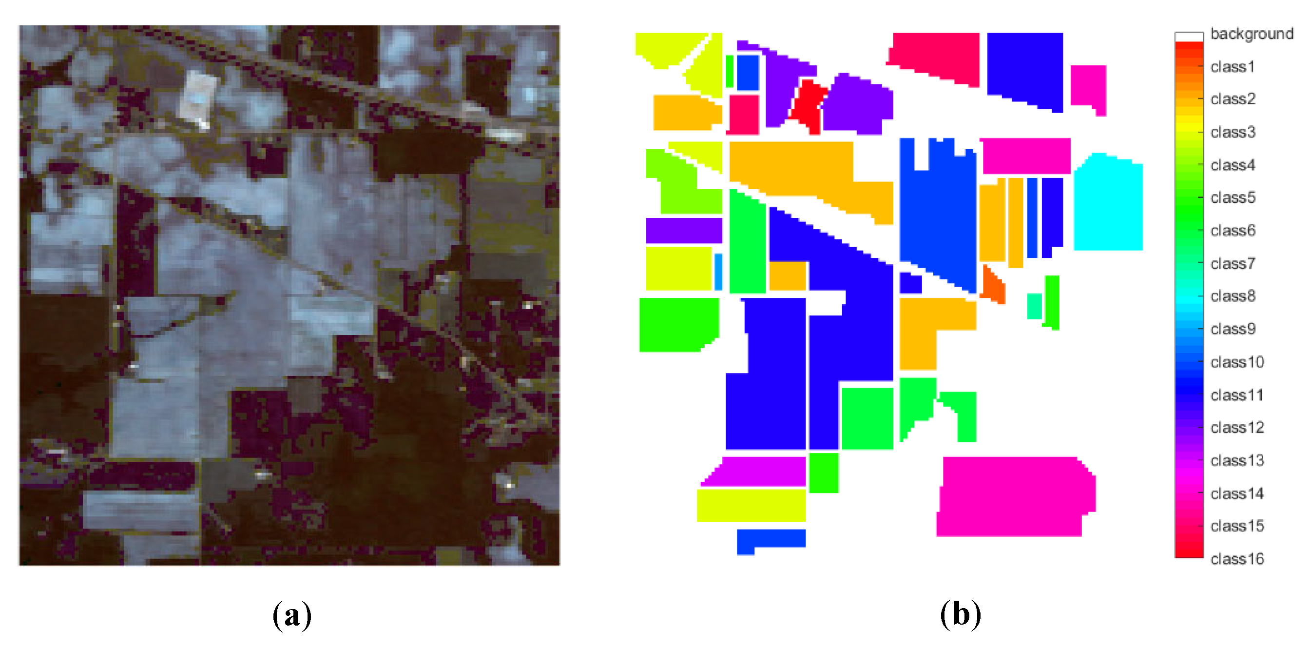
The Indian Pines (IP) dataset was gathered in 1992 by the AVIRIS sensor over the Indian Pines test site in northwest Indiana, United States. The size of the image is pixels and 220 spectral reflectance bands in the wavelength ranges from 0.40 to 2.50 . The spatial resolution is about 20 m. The available ground truth is designated into sixteen classes. The gray image and the reference land-cover map of the Indian Pines are shown in Figure 2. The land cover types with the number of samples are shown in Table 1.

Figure 2.
The Indian Pines dataset. (a) RGB image (band 10, 20, 30). (b) Reference land-cove map (16 classes).

Table 1.
Land cover type with the number of samples for the Indian Pines dataset.
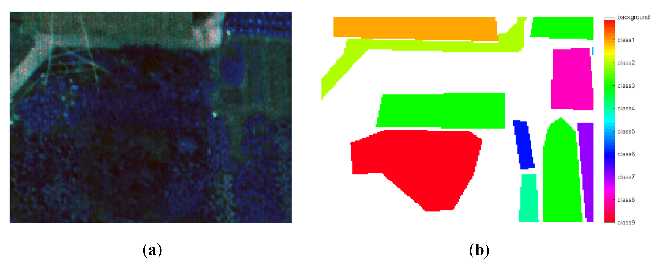
The Pavia University (PU) dataset was collected by the Reflective Optics System Imaging Spectrometer sensor during a flight campaign over the University of Pavia in Pavia, northern Italy. The size of the image was pixels. The spectral reflectance bands were 103 in the wavelength range from 0.43 to 0.86 . The geometric resolution was about 1.3 m. A part of the image with a size of pixels was selected in our experiment. The gray image and the reference land-cover map of the Pavia University are shown in Figure 3. The land cover types with the number of samples are shown in Table 2.
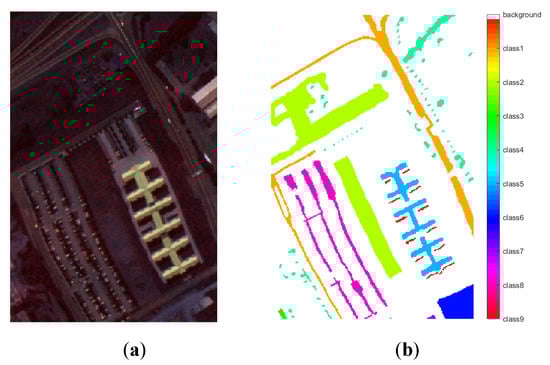
Figure 3.
The Pavia University dataset. (a) RGB image (band 1,20,40). (b) Reference land-cover map (nine classes).
Table 2.
Land cover classes with the number of samples for the Pavia University dataset.
The WHU-Hi-HongHu (HH) dataset [61] was acquired in 2017 in Honghu City, Hubei Province, China, with a 17-mm focal length Headwall Nano-Hyperspec imaging sensor equipped on a DJI Matrice 600 Pro UAV platform. The size of the image was pixels. There were 270 bands from 0.40 to 1.00 . The spatial resolution was about 0.043 m. A part of the image with a size of pixels was selected in our experiment. The gray image and reference land-cover of the WHU-Hi-HongHu dataset are shown in Figure 4. The land cover types with the number of samples are shown in Table 3.

Figure 4.
The WHU-Hi-HongHu dataset. (a) RGB image (band 1,30,60). (b) Reference land-cover map (nine classes).
Table 3.
Land cover classes with the number of samples for Pavia University dataset.
3.2. Experimental Setup
In order to evaluate the performance of the proposed method, three different types of HSIs (including two nature crops scenarios and one urban scenario) were conducted as part of the experiment. Consistent comparisons between CLAP based on the Euclidean distance (ED), the center-based unsupervised algorithms such as the K-means, K-mediods, Spectral clustering (SC) [62], AP as well as Gaussian mixture models (GMM) [63], DBSCAN [64], density peaks clustering (DPC) [65], self-organizing maps (Self-org) [66], competitive layers (CL) [67], HESSC [25], and GR-RSCNet [28] have been carried out. The estimations of the clustering performance provided by these algorithms are given by normalized mutual information (NMI) [68,69], F-measure [39], accuracy (ACC), and adjusted rand index (ARI), which are described as follows.
The mutual information was used to measure the information shared by two clusters and assess their similarity. Given dataset D with N samples and two clusterings of D, namely with R clusters, and with C clusters, the entropy of a cluster U can be defined as
where is the probability of an object falls into cluster and can be defined as . Similarly, the entropy of the clustering can be calculated as
The mutual information between and can be described as
where denotes the probability that a point belongs to cluster in and cluster in . The normalized version of the mutual information can be defined as
The F-measure is an agglomerative method to compare the overall set of clusters. Given cluster and , the F-measure of these clusters is defined as
where is the recall value, and is the precision value. The F-measure of the entire clustering solution is defined as the sum of the maximum F-measure of the individual cluster weighted by the cluster size, which can be expressed as
The cluster accuracy and adjusted Rand index are measurements used to evaluate clustering results. The cluster accuracy can be expressed as
where indicates the best class of labels to reassign, and is the indicator function and can be expressed as
To obtain the adjusted Rand index, we first defined TP, TN, FP, FN. TP denotes the number of pairs of samples that are in the same cluster in U and are also in the same cluster in V; TN denotes the number of pairs of samples that are not in the same cluster in U and are not in the same cluster in V; FP denotes the number of pairs of samples that are not in the same cluster in U, but are in the same cluster in V; FN denotes the number of pairs of samples that are in the same cluster in U, but are not in the same cluster in V. We can define the Rand index as
where denotes the total number of pairs of samples that can be composed in the dataset. The ARI can be expressed as
where is the expected index of the Rand index.
3.3. Experimental Results in Different HSIs
In this experiment, the proposed method and the competitors were conducted on three HSI datasets. For the proposed CLAP, we carried out the experiment with ,, , and . The size of the neighborhood block was pixels (). We decomposed the images using a complex version of a 1-scale, 16-orientation steerable pyramid decomposition, and window. The k-distance of LOF was set to 10. The exemplar preference of CLAP and traditional AP is in the range of , where is the mean value of the pixel distance of the samples. In practice, the pixel distance is obtained by the ED and is normalized to . As a result, the value of is in the range , which was less than 200. For the GR-RSCNet, the learning rate was set to 0.002, and the maximum training epoch was set to 20. The other parameters were set according to [28]. The parameters of other competitors were set according to the corresponding references.
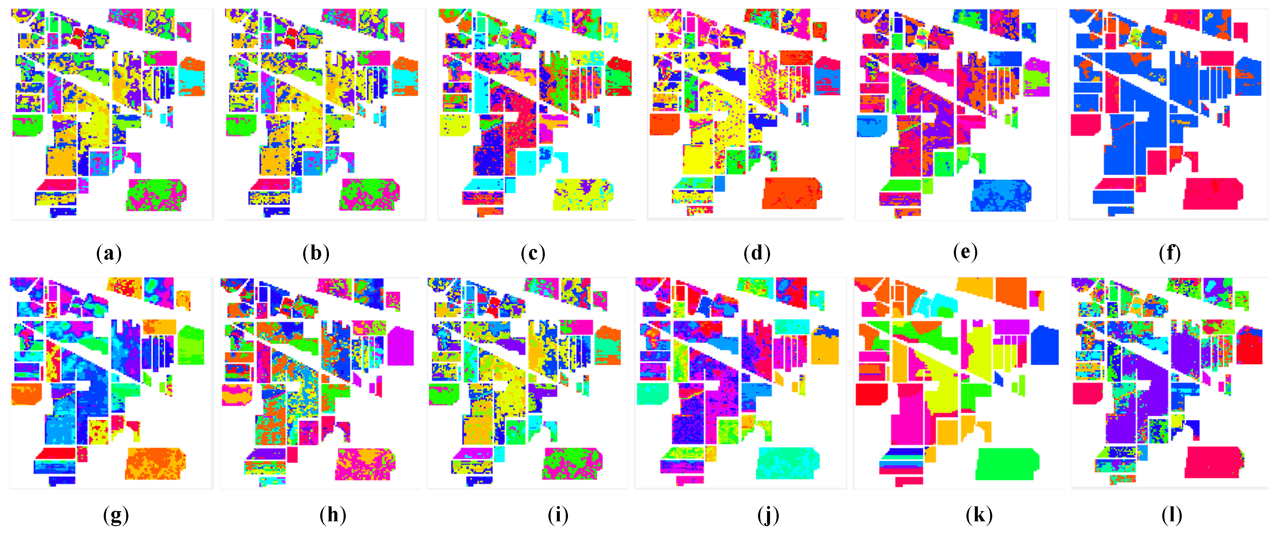
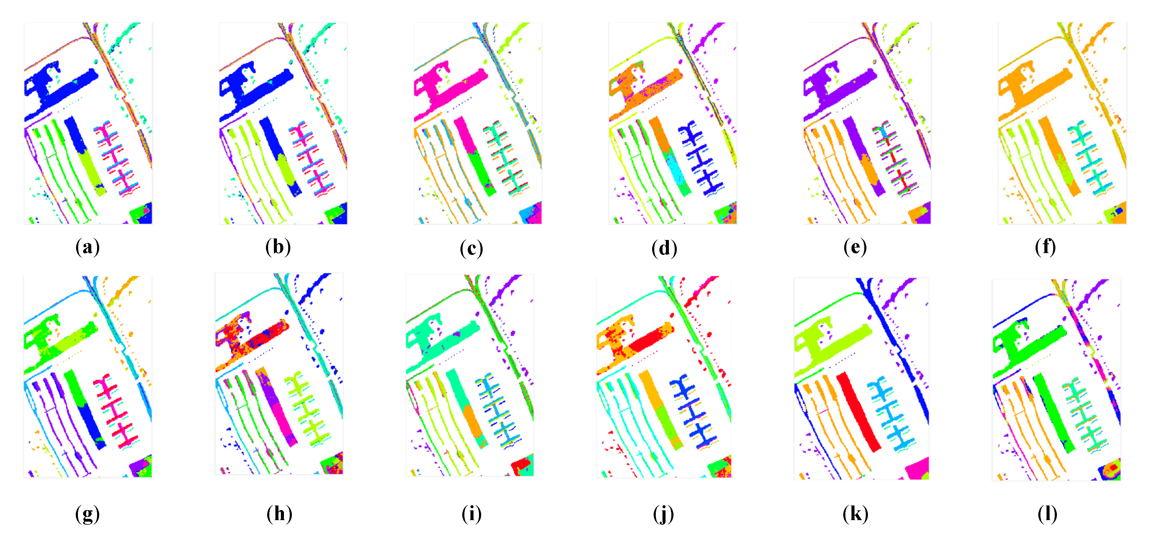
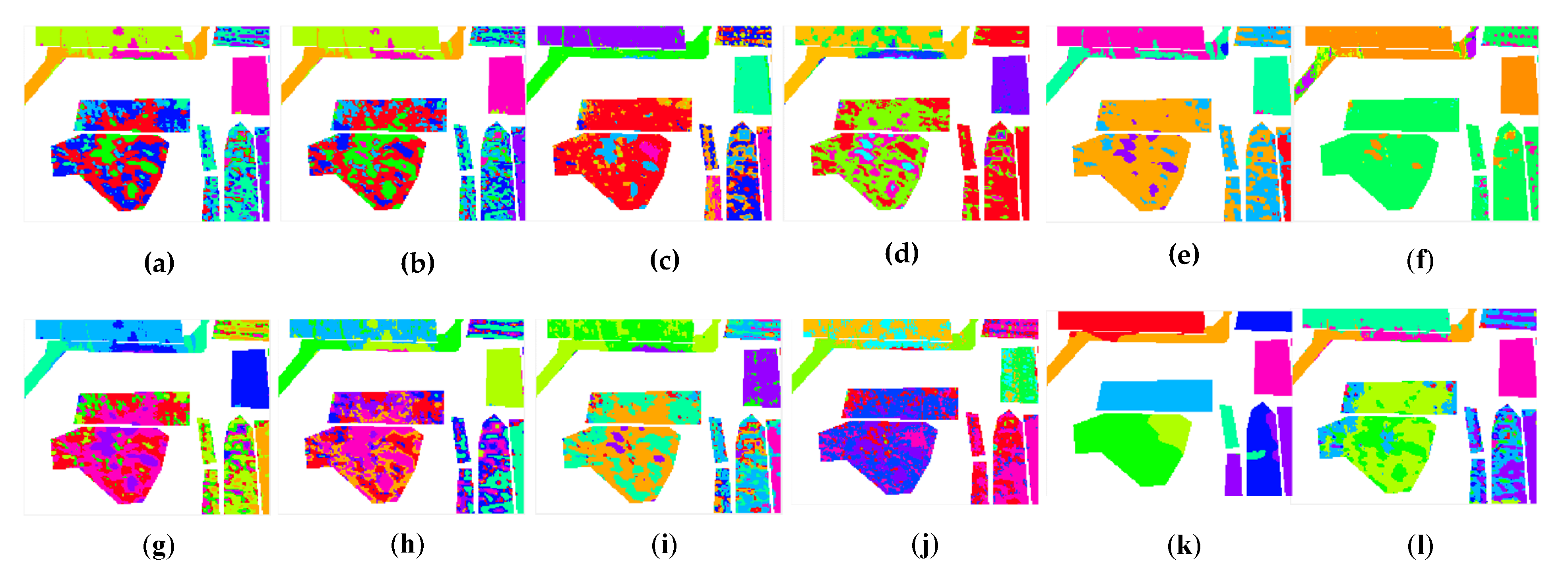
From the comparison between the proposed CLAP and the other clustering methods, we observed that the proposed method was able to achieve the competitive performance in all considered datasets in Figure 5, Figure 6 and Figure 7. The number of mistaken clustering was obviously reduced in Figure 5l, Figure 6l, and Figure 7l. In Figure 5, the proposed method had a better clustering effect on Class 8, Class 13, and Class 14 in the clustering maps of the IP dataset than the competitive method, except for DPC and GR-RSCNet. However, we noticed that the DPC grouped the pixels from different land-covers into the same cluster. The clustering results were obviously unreasonable. Similar phenomena of the clustering results of DPC can be seen in Figure 6f and Figure 7f. Regarding GR-RSCNet, it is the state-of-the-art deep learning-based clustering method, which obtains significantly better clustering results than the traditional clustering algorithms. The same advantage of the proposed method can be seen in Class 2 in the clustering maps of the PU dataset in Figure 6, and on Class 1 and Class 7 in the clustering maps of the HH dataset in Figure 7. The experimental results demonstrate that our proposed method better serves the clustering task and can distinguish different types of land information well. Furthermore, as can be seen from the clustering maps, the proposed CLAP can effectively alleviate the salt-and-pepper phenomenon of the clustering result of the ground objects. Particularly for the HH dataset, the pepper phenomenon of Class 2 and Class 9 was obviously reduced in Figure 7l compared with the clustering results of the competitors except for GR-RSCNet. The main reason is that CLAP invites the spatial information to construct the similarity matrix of the pixels, while the competitors only use the spectral features to achieve the similarity.
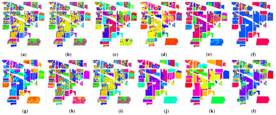
Figure 5.
The clustering maps of the Indian Pines dataset. (a) K-means. (b) K-methods. (c) GMM. (d) DBSCAN. (e) SC. (f) DPC. (g) Self-org. (h) CL. (i) AP. (j) HESSC. (k) GR-RSCNet. (l) CLAP.

Figure 6.
The unsupervised clustering maps of the Pavia University dataset. (a) K-means. (b) K-methods. (c) GMM. (d) DBSCAN. (e) SC. (f) DPC. (g) Self-org. (h) CL. (i) AP. (j) HESSC. (k) GR-RSCNet. (l) CLAP.
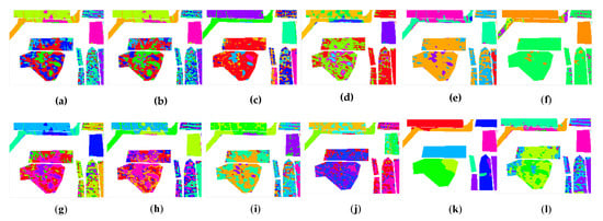
Figure 7.
The unsupervised clustering maps of the WHU-Hi-HongHu dataset. (a) K-means. (b) K-methods. (c) GMM. (d) DBSCAN. (e) SC. (f) DPC. (g) Self-org. (h) CL. (i) AP. (j) HESSC. (k) GR-RSCNet. (l) CLAP.
In order to quantitatively compare the clustering performance, the NMI, F-measure, ACC, and ARI were used to evaluate the algorithms. We collected the average value of the 10 times clustering results of all the algorithms in the three HSI datasets. The results are shown in Table 4.
Table 4.
Comparison results of the NMI, F-measure, ACC, ARI, and running time of the algorithms in three HSI datasets.
In Table 4, we can see that CLAP provided competitive clustering results in all HSI datasets. For the IP dataset, the NMI of CLAP was 0.4525, which was higher than that of the competitors, except for GR-RSCNet. Similarly, the ARI of CLAP (0.3237) was the second highest among the competitors. We noted that the FM and ACC of the DPC was higher than that of CLAP. However, it can be seen from Figure 5f that the clustering result of DPC was inappropriate compared to the real land-cover. Similar conclusions can be obtained for the PU dataset and HH dataset. GMM provided the second-best clustering results in the HH dataset. The CLAP obtained the third-best clustering results in the HH dataset and indicates that the HH dataset is more suitable to be clustered by GMM. The GR-RSCNet obtained the best clustering results among the competitors and showed that the potential of the deep learning-based clustering methods was significantly greater than that of the traditional clustering methods. More specifically, we focused on the comparison of the proposed CLAP with the AP. It can be seen that CLAP provided higher clustering results on all datasets than that of AP and shows that CLAP can effectively improve the performance of the original AP. In addition, we could see that CLAP required more running time than that of the AP. The additional running time was used to calculate the CW-SSIM and LOF. The GR-RSCNet provided the longest running time among the competitors.
3.4. The Optimization Strategy of , , and
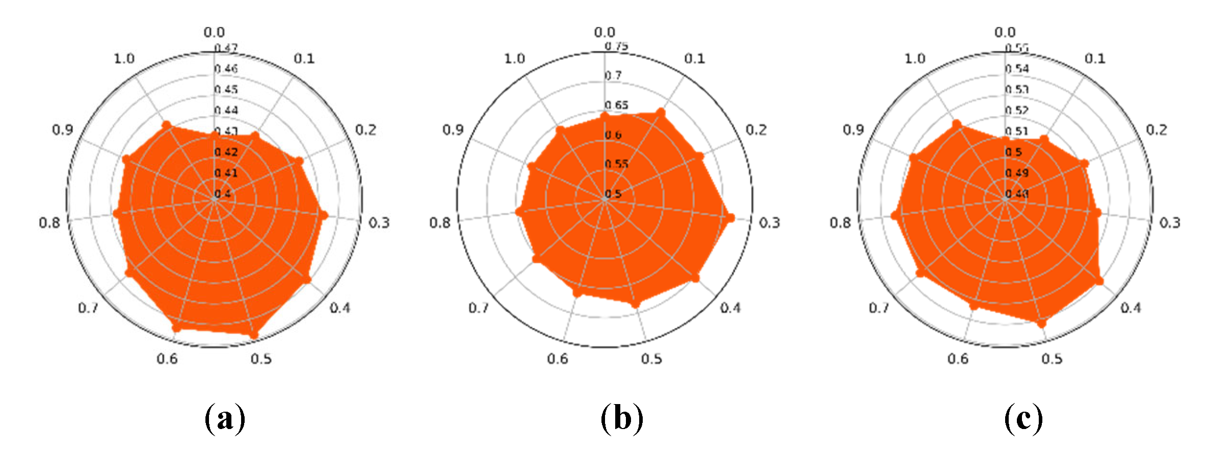
In this section, the settings of parameters, , , and in our CLAP are discussed. To achieve the best clustering performance, these parameters were tuned according to the results of our proposed algorithm running on the HSI datasets. Concerning different values of , which varied from 0 to 1, the clustering precision of the CLAP on the three datasets are shown in Figure 8a–c. It should be noted that is the weight of the spatial structure similarity of ground objects according to Equation (17). Specifically, when is set to 0, the proposed CLAP is simplified to the original AP with only the LOF weighted term. Figure 8a shows that the best clustering result was obtained when the preference selection of α was around 0.5 on the IP dataset. In Figure 8b,c, it can be observed that on the PU dataset, it was around 0.3, and on the HH dataset, it was 0.4, respectively. Furthermore, it should be clearly observed that due to adding the weight term , the clustering performance of the proposed CLAP was better than original AP algorithm (). At the same time, through comparative analysis, it can be found that taking a large value (e.g., is set to greater than 0.8.) may result in that the modified fusion distance (in Equation (17)) depends more on spectral similarity, which in turn reduces the clustering accuracy of the algorithm. This may be because the over-weighted spatial similarity exceeded the threshold of the spectral similarity, introducing too much spatial information, which affects the clustering precision.

Figure 8.
The impact of on the proposed CLAP. (a) Indian Pines dataset. (b) Pavia University dataset. (c) WHU-Hi-HongHu dataset.
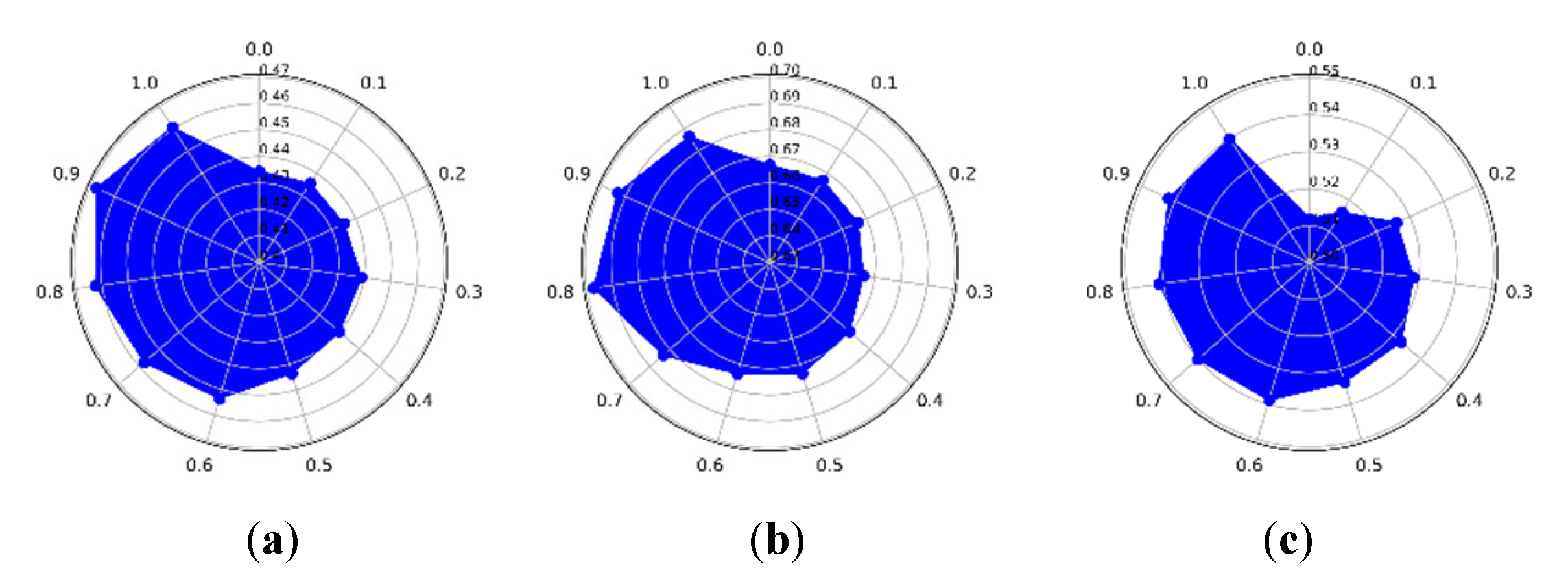
Concerning different values of , which varies from 0 to 1, the clustering precision of the CLAP on the three datasets are shown in Figure 9a–c. According to Equation (19), is the weight of in the LOF coefficient, which is related to estimate suitable exemplar preference. Figure 9a shows that the best clustering result was obtained when the preference selection of was around 0.9 on the IP dataset. From Figure 9b,c it can be observed that it was around 0.8 on both the PU dataset and HH dataset. The experimental results show that a larger is better for estimating suitable exemplar preference.
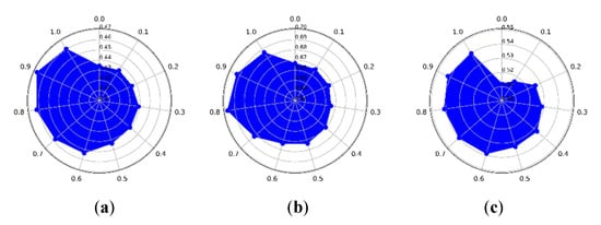
Figure 9.
The impact of on the proposed CLAP. (a) Indian Pines dataset. (b) Pavia University dataset. (c) WHU-Hi-HongHu dataset.
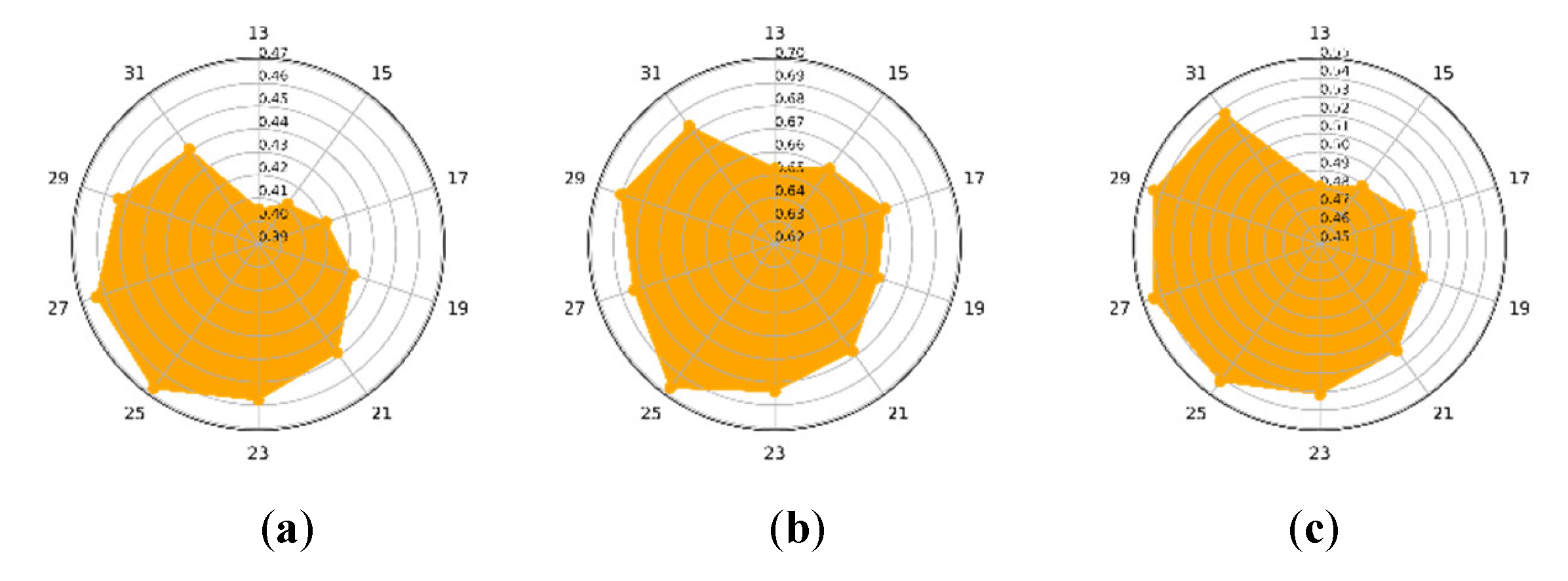
Concerning different values of , which is the size of the spatial neighbourhood block and varies from 13 to 31, the clustering precision of CLAP on the three datasets are shown in Figure 10a–c. Figure 10a shows that on the IP dataset, when the is set to about 25 (i.e., the size of block is pixels), the best clustering result was obtained. Similarly, in Figure 10b,c, it can be observed that on the PU dataset, it was and on the HH dataset, it was , respectively. The experimental results show that its value of is too small (eg. ), which can result in the poor clustering performance. It may be because too small a block may result in missing useful structural information, which in turn will reduce the clustering performance.
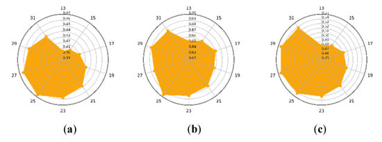
Figure 10.
The influence of . (a) Indian Pines dataset. (b) Pavia University dataset. (c) WHU-Hi-HongHu dataset.
4. Discussion
In this paper, the structural similarity index and local outlier factor were introduced to improve the original AP clustering. Comparisons were conducted on three HSI datasets. The visual and statistical results are shown in Figure 5, Figure 6 and Figure 7 and Table 4. The influence of the parameters is discussed in Section 3.4.
From the clustering results of CLAP and AP, we can see that CLAP provided better results than AP on all three HSI datasets. It is understandable that we collected more information from the HSI dataset in CLAP. The CW-SSIM can be denoted as spatial information. The LOF can be denoted as spectral information and indicates that the extraction of the spatial-spectral information of the HSI dataset can effectively improve the performance of the clustering algorithms. This practice gives us an idea of how to improve the algorithms for processing the HSI dataset. Although CLAP requires a longer running time than that of AP, the improved strategy for calculating the CW-SSIM distance is still in effect, where the running time was significantly reduced compared to the direct usage of CW-SSIM between a pair of spatial neighborhood blocks. For example, the running time of the original CW-SSIM distance strategy was more than five hours on the IP dataset, and that of the improved version was about 290 s.
Furthermore, broader comparisons were conducted in the experiment. From the comparison results, we can see that the proposed CLAP provided competitive clustering performance, which was in the top three in all indicators on three HSI datasets. The deep learning-based clustering method provided the best clustering result among the competitors, which showed great potential to address the issue of the HSI clustering. However, the deep learning-based clustering method provided the highest running time (the running time was obtained on the GPU platform of Tesla V100 16G) than that of the traditional clustering methods (the running time was obtained on the CPU platform of Intel Core i5-6200U). There is still interesting work to improve the efficiency of the deep learning-based clustering method.
Meanwhile, there are still some drawbacks to the proposed CLAP. First, the proposed CLAP has many parameters to be modulated such as . The optimal values of these parameters vary according to the dataset. To simplify the optimization, we provided a set of initial parameters () designed to help optimize the parameters. Experiments showed that satisfactory results can be obtained by selecting parameters around the initial parameters. Second, CW-SSIM was used to extract the structure-based spatial similarity of the HSI dataset. Experiments showed that it had poor performance of spatial similarity, which needs to precisely control the weighting of the spatial similarity. Finally, CLAP requires a global similarity matrix to transfer information between samples. The global similarity matrix needs large storage space to store a large scale HSI dataset.
5. Conclusions
In this paper, a modified AP based on CW-SSIM and LOF was proposed. The CW-SSIM was used to extract the structure-based spatial similarity of the HSI dataset, which was combined with the pixel-based spectral similarity to generate the final similarity matrix of AP. The LOF was applied to measure the smoothness of an object and used to revise the exemplar preference of AP. Meanwhile, we simplified the calculation of the spatial similarity to reduce the computational complexity. The modified similarity matrix was obtained by the pixel-based spectral similarity, the structure-based spatial similarity, and the revised exemplar preference. Finally, the modified similarity matrix was applied to AP and the clustering index was obtained.
To evaluate the effectiveness of the proposed CLAP, comparisons were carried out between CLAP, AP, K-means, K-methods, GMM, DBSCAN, SC, DPC, Self-org, CL, HESSC, and GR-RSCNet on three different types of HSI datasets. The experimental results showed that the proposed CLAP could distinguish different types of land covers well and outperformed its competitors. Meanwhile, the optimization strategy of the main parameters of CLAP was also discussed. From the clustering results, we can see that the weight of spatial similarity should be tuned carefully as too large values may reduce the clustering precision of the algorithm. The weight of the LOF coefficient and the size of the spatial neighborhood block also have an impact on the clustering result. The comparison and drawbacks are discussed in the Discussion section. We can see that CLAP outperformed its competitors, but still suffers from some issues such as difficulty in selecting parameters, unstable performance of the CW-SSIM, and high storage requirements. Further work will focus on the improvement in the scheme to efficiently extract the spatial-spectral information of the HSI dataset in combination with deep learning-based HSI clustering algorithms.
Author Contributions
Conceptualization, H.G.; Data curation, H.G., H.P., Y.Z., X.Z. and M.L.; Formal analysis, H.G., H.P., Y.Z., X.Z. and M.L.; Funding acquisition, H.G. and L.W.; Investigation, H.G., H.P., Y.Z., X.Z. and M.L.; Methodology, H.G.; Project administration, H.G. and L.W.; Resources, H.G. and L.W.; Software, H.G.; Supervision, H.G. and L.W.; Validation, H.G.; Visualization, H.G.; Writing—original draft, H.G.; Writing—review & editing, H.G., L.W., H.P., Y.Z., X.Z. and M.L. All authors have read and agreed to the published version of the manuscript.
Funding
This research was funded by the National Natural Science Foundation of China, grant number 62071084 and the Fundamental Research Funds in Heilongjiang Provincial Universities, grant number 145109218.
Institutional Review Board Statement
Not applicable.
Informed Consent Statement
Not applicable.
Data Availability Statement
Not applicable.
Acknowledgments
The authors would like to thank the associate Editor and the two anonymous reviewers for their constructive comments that have improved the manuscript.
Conflicts of Interest
The authors declare no conflict of interest.
Abbreviations
The following abbreviations are used in this manuscript:
| HIS | Hyperspectral image |
| AP | Affinity propagation |
| SSIM | Structural similarity |
| CW-SSIM | Complex wavelet structural similarity |
| LOF | Local outlier factor |
| CLAP | Improved AP with CW-SSIM and LOF |
| PCA | Principal component analysis |
| PC | Principal component |
| IP | Indian Pines dataset |
| PU | Pavia University dataset |
| HH | WHU-Hi-HongHu dataset |
| ED | Euclidean distance |
| SC | Spectral clustering |
| GMM | Gaussian mixture models |
| DPC | Density peaks clustering |
| Self-org | Self-organizing maps |
| CL | Competitive layers |
| HESSC | Hierarchical sparse subspace clustering |
| GR-RSCNet | Graph regularized residual subspace clustering network |
| NMI | Normalized mutual information |
| ACC | Accuracy |
| ARI | Adjusted rand index |
References
- Ou, D.P.; Tan, K.; Du, Q.; Zhu, J.S.; Wang, X.; Chen, Y. A Novel Tri-Training Technique for the Semi-Supervised Classification of Hyperspectral Images Based on Regularized Local Discriminant Embedding Feature Extraction. Remote Sens. 2019, 11, 654. [Google Scholar] [CrossRef] [Green Version]
- Chung, B.; Yu, J.; Wang, L.; Kim, N.H.; Lee, B.H.; Koh, S.; Lee, S. Detection of Magnesite and Associated Gangue Minerals using Hyperspectral Remote Sensing-A Laboratory Approach. Remote Sens. 2020, 12, 1325. [Google Scholar] [CrossRef] [Green Version]
- Shimoni, M.; Haelterman, R.; Perneel, C. Hyperspectral Imaging for Military and Security Applications Combining myriad processing and sensing techniques. IEEE Geosci. Remote Sens. Mag. 2019, 7, 101–117. [Google Scholar] [CrossRef]
- Chehdi, K.; Soltani, M.; Cariou, C. Pixel classification of large-size hyperspectral images by affinity propagation. J. Appl. Remote Sens. 2014, 8, 083567. [Google Scholar] [CrossRef] [Green Version]
- Zhai, H.; Zhang, H.Y.; Li, P.X.; Zhang, L.P. Hyperspectral Image Clustering: Current Achievements and Future Lines. IEEE Geosci. Remote Sens. Mag. 2021, 9, 35–67. [Google Scholar] [CrossRef]
- Jain, A.K. Data clustering: 50 years beyond K-means. Pattern Recognit. Lett. 2010, 31, 651–666. [Google Scholar] [CrossRef]
- Kanungo, T.; Mount, D.M.; Netanyahu, N.S.; Piatko, C.D.; Silverman, R.; Wu, A.Y. An efficient k-means clustering algorithm: Analysis and implementation. Ieee Trans. Pattern Anal. Mach. Intell. 2002, 24, 881–892. [Google Scholar] [CrossRef]
- Wong, J.A.H.A. Algorithm AS 136: A K-Means Clustering Algorithm. J. R. Stat. Soc. 1979, 28, 100–108. [Google Scholar]
- Ros, F.; Guillaume, S. DENDIS: A new density-based sampling for clustering algorithm. Expert Syst. Appl. 2016, 56, 349–359. [Google Scholar] [CrossRef] [Green Version]
- Tao, X.M.; Guo, W.J.; Ren, C.; Li, Q.; He, Q.; Liu, R.; Zou, J.R. Density peak clustering using global and local consistency adjustable manifold distance. Inf. Sci. 2021, 577, 769–804. [Google Scholar] [CrossRef]
- Rodriguez, A.; Laio, A. Clustering by fast search and find of density peaks. Science 2014, 344, 1492–1496. [Google Scholar] [CrossRef] [Green Version]
- Fraley, C.; Raftery, A.E. Model-based clustering, discriminant analysis, and density estimation. J. Am. Stat. Assoc. 2002, 97, 611–631. [Google Scholar] [CrossRef]
- Reynolds, D.A.; Quatieri, T.F.; Dunn, R.B. Speaker verification using adapted Gaussian mixture models. Digit. Signal. Processing 2000, 10, 19–41. [Google Scholar] [CrossRef] [Green Version]
- Fakoor, D.; Maihami, V.; Maihami, R. A machine learning recommender system based on collaborative filtering using Gaussian mixture model clustering. In Mathematucal Methods in the Applied Science; Wiley Online Library: Hoboken, NJ, USA, 2021. [Google Scholar] [CrossRef]
- Fuchs, R.; Pommeret, D.; Viroli, C. Mixed Deep Gaussian Mixture Model: A clustering model for mixed datasets. Adv. Data Anal. Classif. 2021, 1–23. [Google Scholar] [CrossRef]
- Jiao, H.; Zhong, Y.; Zhang, L. An unsupervised spectral matching classifier based on artificial DNA computing for hyperspectral remote sensing imagery. IEEE Trans. Geosci. Remote Sens. 2013, 52, 4524–4538. [Google Scholar] [CrossRef]
- Zhong, Y.; Zhang, L.; Huang, B.; Li, P. An unsupervised artificial immune classifier for multi/hyperspectral remote sensing imagery. IEEE Trans. Geosci. Remote Sens. 2006, 44, 420–431. [Google Scholar] [CrossRef]
- Zhong, Y.; Zhang, S.; Zhang, L. Automatic fuzzy clustering based on adaptive multi-objective differential evolution for remote sensing imagery. IEEE J. Sel. Top. Appl. Earth Obs. Remote Sens. 2013, 6, 2290–2301. [Google Scholar] [CrossRef]
- Ma, A.; Zhong, Y.; Zhang, L. Adaptive multiobjective memetic fuzzy clustering algorithm for remote sensing imagery. IEEE Trans. Geosci. Remote Sens. 2015, 53, 4202–4217. [Google Scholar] [CrossRef]
- Zhu, W.; Chayes, V.; Tiard, A.; Sanchez, S.; Dahlberg, D.; Bertozzi, A.L.; Osher, S.; Zosso, D.; Kuang, D. Unsupervised classification in hyperspectral imagery with nonlocal total variation and primal-dual hybrid gradient algorithm. IEEE Trans. Geosci. Remote Sens. 2017, 55, 2786–2798. [Google Scholar] [CrossRef]
- Liu, W.; Li, S.; Lin, X.; Wu, Y.; Ji, R. Spectral–spatial co-clustering of hyperspectral image data based on bipartite graph. Multimed. Syst. 2016, 22, 355–366. [Google Scholar] [CrossRef]
- Zhai, H.; Zhang, H.; Xu, X.; Zhang, L.; Li, P. Kernel sparse subspace clustering with a spatial max pooling operation for hyperspectral remote sensing data interpretation. Remote Sens. 2017, 9, 335. [Google Scholar] [CrossRef] [Green Version]
- Zhang, H.; Zhai, H.; Zhang, L.; Li, P. Spectral–spatial sparse subspace clustering for hyperspectral remote sensing images. IEEE Trans. Geosci. Remote Sens. 2016, 54, 3672–3684. [Google Scholar] [CrossRef]
- Tian, L.; Du, Q.; Kopriva, I.; Younan, N. Spatial-spectral Based Multi-view Low-rank Sparse Sbuspace Clustering for Hyperspectral Imagery. In Proceedings of the IGARSS 2018—2018 IEEE International Geoscience and Remote Sensing Symposium, Valencia, Spain, 22–27 July 2018; pp. 8488–8491. [Google Scholar]
- Shahi, K.R.; Khodadadzadeh, M.; Tusa, L.; Ghamisi, P.; Tolosana-Delgado, R.; Gloaguen, R. Hierarchical Sparse Subspace Clustering (HESSC): An Automatic Approach for Hyperspectral Image Analysis. Remote Sens. 2020, 12, 2421. [Google Scholar] [CrossRef]
- Hsu, C.-C.; Lin, C.-W. Cnn-based joint clustering and representation learning with feature drift compensation for large-scale image data. IEEE Trans. Multimed. 2017, 20, 421–429. [Google Scholar] [CrossRef] [Green Version]
- Yang, B.; Fu, X.; Sidiropoulos, N.D.; Hong, M. Towards k-means-friendly spaces: Simultaneous deep learning and clustering. In Proceedings of the 34th International Conference on Machine Learning, Sydney, Australia, 6–11 August 2017; PMLR: New York City, NY, USA, 2017; Volume 70, pp. 3861–3870. [Google Scholar]
- Cai, Y.M.; Zeng, M.; Cai, Z.H.; Liu, X.B.; Zhang, Z.J. Graph Regularized Residual Subspace Clustering Network for hyperspectral image clustering. Inf. Sci. 2021, 578, 85–101. [Google Scholar] [CrossRef]
- Xie, H.; Zhao, A.; Huang, S.; Han, J.; Liu, S.; Xu, X.; Luo, X.; Pan, H.; Du, Q.; Tong, X. Unsupervised hyperspectral remote sensing image clustering based on adaptive density. IEEE Geosci. Remote Sens. Lett. 2018, 15, 632–636. [Google Scholar] [CrossRef]
- Neagoe, V.-E.; Chirila-Berbentea, V. Improved Gaussian mixture model with expectation-maximization for clustering of remote sensing imagery. In Proceedings of the 2016 IEEE International Geoscience and Remote Sensing Symposium (IGARSS), Beijing, China, 10–15 July 2016; pp. 3063–3065. [Google Scholar]
- Frey, B.J.; Dueck, D. Clustering by passing messages between data points. Science 2007, 315, 972–976. [Google Scholar] [CrossRef] [Green Version]
- Dagher, I.; Mikhael, S.; Al-Khalil, O. Gabor face clustering using affinity propagation and structural similarity index. Multimed. Tools Appl. 2021, 80, 4719–4727. [Google Scholar] [CrossRef]
- Ge, H.; Pan, H.; Wang, L.; Li, C.; Liu, Y.; Zhu, W.; Teng, Y. A semi-supervised learning method for hyperspectral imagery based on self-training and local-based affinity propagation. Int. J. Remote Sens. 2021, 42, 6391–6416. [Google Scholar] [CrossRef]
- Li, M.; Wang, Y.X.; Chen, Z.G.; Zhao, J. Intelligent fault diagnosis for rotating machinery based on potential energy feature and adaptive transfer affinity propagation clustering. Meas. Sci. Technol. 2021, 32, 094012. [Google Scholar] [CrossRef]
- Liu, J.J.; Kan, J.Q. Recognition of genetically modified product based on affinity propagation clustering and terahertz spectroscopy. Spectrochim. Acta Part A-Mol. Biomol. Spectrosc. 2018, 194, 14–20. [Google Scholar] [CrossRef] [PubMed]
- Liu, J.X.; Yu, D.; Tang, Z. Video summary generation by visual shielding compressed sensing coding and double-layer affinity propagation. J. Vis. Commun. Image Represent. 2021, 81, 103321. [Google Scholar] [CrossRef]
- Zhang, Y.J.; Deng, J.; Zhu, K.K.; Tao, Y.Q.; Liu, X.L.; Cui, L.G. Location and Expansion of Electric Bus Charging Stations Based on Gridded Affinity Propagation Clustering and a Sequential Expansion Rule. Sustainability 2021, 13, 8957. [Google Scholar] [CrossRef]
- Wan, X.J.; Li, H.L.; Zhang, L.P.; Wu, Y.J. Multivariate Time Series Data Clustering Method Based on Dynamic Time Warping and Affinity Propagation. Wirel. Commun. Mob. Comput. 2021, 2021, 9915315. [Google Scholar] [CrossRef]
- Wang, L.M.; Ji, Q.; Han, X.M. Aaptive semi-supervised affinity propagation clustering algorithm based on structural similarity. Teh. Vjesn.-Tech. Gaz. 2016, 23, 425–435. [Google Scholar] [CrossRef] [Green Version]
- Zhang, W.; Wu, X.F.; Zhu, W.P.; Yu, L. Unsupervized Image Clustering With SIFT-Based Soft-Matching Affinity Propagation. Ieee Signal. Processing Lett. 2017, 24, 461–464. [Google Scholar] [CrossRef]
- Qin, Y.; Li, B.; Ni, W.; Quan, S.; Bian, H. Affinity Matrix Learning Via Nonnegative Matrix Factorization for Hyperspectral Imagery Clustering. IEEE J. Sel. Top. Appl. Earth Obs. Remote Sens. 2020, 14, 402–415. [Google Scholar] [CrossRef]
- Fan, L.; Messinger, D.W. Joint spatial-spectral hyperspectral image clustering using block-diagonal amplified affinity matrix. Opt. Eng. 2018, 57. [Google Scholar] [CrossRef]
- Chen, D.W.; Sheng, J.Q.; Chen, J.J.; Wang, C.D. Stability-based preference selection in affinity propagation. Neural Comput. Appl. 2014, 25, 1809–1822. [Google Scholar] [CrossRef]
- Gan, G.J.; Ng, M.K.P. Subspace clustering using affinity propagation. Pattern Recognit. 2015, 48, 1455–1464. [Google Scholar] [CrossRef]
- Li, P.; Ji, H.F.; Wang, B.L.; Huang, Z.Y.; Li, H.Q. Adjustable preference affinity propagation clustering. Pattern Recognit. Lett. 2017, 85, 72–78. [Google Scholar] [CrossRef]
- Hu, J.S.; Liu, H.L.; Yan, Z. Adaptive Affinity Propagation Algorithm Based on New Strategy of Dynamic Damping Factor and Preference. Ieej Trans. Electr. Electron. Eng. 2019, 14, 97–104. [Google Scholar] [CrossRef] [Green Version]
- Wang, Z.; Bovik, A.C.; Sheikh, H.R.; Simoncelli, E.P. Image quality assessment: From error visibility to structural similarity. Ieee Trans. Image Processing 2004, 13, 600–612. [Google Scholar] [CrossRef] [PubMed] [Green Version]
- Sampat, M.P.; Wang, Z.; Gupta, S.; Bovik, A.C.; Markey, M.K. Complex wavelet structural similarity: A new image similarity index. IEEE Trans. Image Process. 2009, 18, 2385–2401. [Google Scholar] [CrossRef] [PubMed]
- Rehman, A.; Gao, Y.; Wang, J.H.; Wang, Z. Image classification based on complex wavelet structural similarity. Signal. Processing-Image Commun. 2013, 28, 984–992. [Google Scholar] [CrossRef]
- Rodriguez-Pulecio, C.G.; Benitez-Restrepo, H.D.; Bovik, A.C. Making long-wave infrared face recognition robust against image quality degradations. Quant. Infrared Thermogr. J. 2019, 16, 218–242. [Google Scholar] [CrossRef]
- Jia, S.; Zhu, Z.; Shen, L.; Li, Q. A Two-Stage Feature Selection Framework for Hyperspectral Image Classification Using Few Labeled Samples. IEEE J. Sel. Top. Appl. Earth Obs. Remote Sens. 2014, 7, 1023–1035. [Google Scholar] [CrossRef]
- Casti, P.; Mencattini, A.; Salmeri, M.; Rangayyan, R.M. Analysis of Structural Similarity in Mammograms for Detection of Bilateral Asymmetry. IEEE Trans. Med. Imaging 2015, 34, 662–671. [Google Scholar] [CrossRef] [PubMed]
- Breunig, M.M.; Kriegel, H.P.; Ng, R.T.; Sander, J. LOF: Identifying density-based local outliers. Sigmod Rec. 2000, 29, 93–104. [Google Scholar] [CrossRef]
- Tu, B.; Zhou, C.L.; Kuang, W.L.; Guo, L.Y.; Ou, X.F. Hyperspectral Imagery Noisy Label Detection by Spectral Angle Local Outlier Factor. IEEE Geosci. Remote Sens. Lett. 2018, 15, 1417–1421. [Google Scholar] [CrossRef]
- Zhang, Z.J.; Lan, H.M.; Zhao, T.J. Detection and mitigation of radiometers radio-frequency interference by using the local outlier factor. Remote Sens. Lett. 2017, 8, 311–319. [Google Scholar] [CrossRef]
- Yu, S.Q.; Li, X.R.; Zhao, L.Y.; Wang, J. Hyperspectral Anomaly Detection Based on Low-Rank Representation Using Local Outlier Factor. IEEE Geosci. Remote Sens. Lett. 2021, 18, 1279–1283. [Google Scholar] [CrossRef]
- Ge, H.M.; Pan, H.Z.; Wang, L.G.; Liu, M.Q.; Li, C. Self-training algorithm for hyperspectral imagery classification based on mixed measurement k-nearest neighbor and support vector machine. J. Appl. Remote Sens. 2021, 15, 042604. [Google Scholar] [CrossRef]
- Guo, Z.H.; Zhang, D.; Zhang, L.; Liu, W.H. Feature Band Selection for Online Multispectral Palmprint Recognition. IEEE Trans. Inf. Forensics Secur. 2012, 7, 1094–1099. [Google Scholar] [CrossRef]
- Portilla, J.; Simoncelli, E.P. A parametric texture model based on joint statistics of complex wavelet coefficients. Int. J. Comput. Vis. 2000, 40, 49–71. [Google Scholar] [CrossRef]
- Simoncelli, E.P.; Freeman, W.T.; Adelson, E.H.; Heeger, D.J. Shiftable multiscale transforms. IEEE Trans. Inf. Theory 1992, 38, 587–607. [Google Scholar] [CrossRef] [Green Version]
- Zhong, Y.F.; Hu, X.; Luo, C.; Wang, X.Y.; Zhao, J.; Zhang, L.P. WHU-Hi: UAV-borne hyperspectral with high spatial resolution (H-2) benchmark datasets and classifier for precise crop identification based on deep convolutional neural network with CRF. Remote Sens. Environ. 2020, 250, 112012. [Google Scholar] [CrossRef]
- Von Luxburg, U. A tutorial on spectral clustering. Stat. Comput. 2007, 17, 395–416. [Google Scholar] [CrossRef]
- Reynolds, D.A. Gaussian mixture models. Encycl. Biom. 2009, 741, 659–663. [Google Scholar]
- Birant, D.; Kut, A. ST-DBSCAN: An algorithm for clustering spatial–temporal data. Data Knowl. Eng. 2007, 60, 208–221. [Google Scholar] [CrossRef]
- Du, M.; Ding, S.; Jia, H. Study on density peaks clustering based on k-nearest neighbors and principal component analysis. Knowl.-Based Syst. 2016, 99, 135–145. [Google Scholar] [CrossRef]
- Kohonen, T. Exploration of very large databases by self-organizing maps. In Proceedings of the International Conference on Neural Networks (icnn’97), Houston, TX, USA, 12 June 1997; Volume 1, pp. PL1–PL6. [Google Scholar]
- Steffen, J.; Pardowitz, M.; Steil, J.J.; Ritter, H. Integrating feature maps and competitive layer architectures for motion segmentation. Neurocomputing 2011, 74, 1372–1381. [Google Scholar] [CrossRef]
- Studholme, C.; Hill, D.L.G.; Hawkes, D.J. An overlap invariant entropy measure of 3D medical image alignment. Pattern Recognit. 1999, 32, 71–86. [Google Scholar] [CrossRef]
- Huang, X.H.; Ye, Y.M.; Zhang, H.J. Extensions of Kmeans-Type Algorithms: A New Clustering Framework by Integrating Intracluster Compactness and Intercluster Separation. IEEE Trans. Neural. Netw. Learn. Syst. 2014, 25, 1433–1446. [Google Scholar] [CrossRef] [PubMed]

Publisher’s Note: MDPI stays neutral with regard to jurisdictional claims in published maps and institutional affiliations. |
© 2022 by the authors. Licensee MDPI, Basel, Switzerland. This article is an open access article distributed under the terms and conditions of the Creative Commons Attribution (CC BY) license (https://creativecommons.org/licenses/by/4.0/).