Multiscale Feature Aggregation Capsule Neural Network for Hyperspectral Remote Sensing Image Classification

Abstract

Models based on capsule neural network (CapsNet), a novel deep learning method, have recently made great achievements in hyperspectral remote sensing image (HSI) classification due to their excellent ability to implicitly model the spatial relationship knowledge embedded in HSIs. However, the number of labeled samples is a common bottleneck in HSI classification, limiting the performance of these deep learning models. To alleviate the problem of limited labeled samples and further explore the potential of CapsNet in the HSI classification field, this study proposes a multiscale feature aggregation capsule neural network (MS-CapsNet) based on CapsNet via the implementation of two branches that simultaneously extract spectral, local spatial, and global spatial features to integrate multiscale features and improve model robustness. Furthermore, because deep features are generally more discriminative than shallow features, two kinds of capsule residual (CapsRES) blocks based on 3D convolutional capsule (3D-ConvCaps) layers and residual connections are proposed to increase the depth of the network and solve the limited labeled sample problem in HSI classification. Moreover, a squeeze-and-excitation (SE) block is introduced in the shallow layers of MS-CapsNet to enhance its feature extraction ability. In addition, a reasonable initialization strategy that transfers parameters from two well-designed, pretrained deep convolutional capsule networks is introduced to help the model find a good set of initializing weight parameters and further improve the HSI classification accuracy of MS-CapsNet. Experimental results on four widely used HSI datasets demonstrate that the proposed method can provide results comparable to those of state-of-the-art methods.

1. Introduction

Hyperspectral remote sensing images (HSIs) contain rich spectral and spatial information, which can greatly improve ground object recognition and provide a wide range of applications in many fields [1,2,3,4,5]. In recent decades, various classification methods based on spectral information have been proposed to perform HSI classification tasks, such as random forest (RF) [6], support vector machine (SVM) [7], and k-nearest neighbor (kNN) [8]. HSIs provide abundant spatial information, and their spatial resolution continues to increase with advancements in sensor technology. In the HSI classification field, the introduction of spatial information can significantly improve the robustness of classification methods to noise [9,10,11]. Numerous studies on HSI classification based on spectral-spatial information have been published. Zhao et al. [12] used a band subset-based clustering and fusion technique to utilize the spectral and spatial information from HSIs simultaneously. As improvements continue to be made in SVMs, some effective techniques, such as morphological profiles and multiple kernel learning, have been introduced to accurately obtain the final classification result [13,14]. However, HSI data structures usually present with high-dimensional and highly nonlinear characteristics, which easily cause the Hugh phenomenon for supervised learning methods with limited training samples [10,15].

Deep learning methods, such as stacked autoencoders (SAEs) [16], deep belief networks (DBNs) [17], recurrent neural networks (RNNs) [18], and convolutional neural networks (CNNs) [19,20,21], can automatically extract abstract features from low levels to high levels and achieve accurate HSI classification results. Typically, CNNs dominate the field of HSI image processing due to their characteristics of local reception and weight sharing. For example, in [22], a 1D convolutional neural network (1D-CNN) was proposed to extract pixel-pair features in the spectral domain to explore the correlation between pixels and improve the generalization ability of the model. However, 1D-CNN only uses the eigenvector of the spectral signal as the input data, ignoring much of the spatial information. To make effective use of the rich spatial information in HSIs, the 2D convolutional neural network (2D-CNN) was introduced to extract spectral and spatial information, and dimension reduction algorithms were used to reduce the spectral dimension in the pre-processing stage [23,24]. However, these 2D-CNN–based methods still experience spectral information loss in the image preprocessing stage. Generally, HSI data are represented as a three-dimensional cube that can be sampled in both the spatial and spectral domains simultaneously by using a 3D convolution operation to simultaneously extract spectral and spatial features. To make full use of the spectral and spatial information in HSIs, the 3D convolutional neural network (3D-CNN) was proposed to extract spectral-spatial features and further improve performance in the HSI classification field [25]. Li et al. [26] proposed a lightweight 3D-CNN to classify HSIs that not only used fewer parameters but also greatly improved the classification accuracy over the 2D-CNN and 1D-CNN. Generally, the quality of feature representation is related to the depth of the model, but it is difficult to extract fine deep spectral-spatial features by simply deepening the network through the stacking of convolution layers [27]. In this instance, some effective techniques were introduced to strengthen network information transmission, such as residual [28,29] and dense connections [30,31]. Furthermore, considering the strong complementary relationship between different features, Zhang et al. [32] discussed the influence of different feature aggregation methods on HSI classification and proposed a deep feature residual network (DFRN) and deep feature dense network (DFDN) to fuse low-, middle-, and high-level features, which significantly improved the HSI classification accuracy. Li et al. [33] proposed a two-stream 2D-CNN method to aggregate the spectral-spatial features extracted from multiple inputs, achieving good performance. In addition, CNNs can be combined with other powerful techniques to improve HSI classification performance, such as transfer learning [34], sparse representation [35], metric learning [36], attention techniques [37], and morphological profiles [38]. The performance of a deep learning model is related to the number of training samples. Specifically, the performance is often relatively poor when the number of training samples is limited. To fully utilize the advantages of a CNN, Chen et al. [39] integrated ensemble learning and a CNN in the field of HSI classification, in which the final class of the ground object is determined by voting on several simple CNN models; the final model achieves a good classification result. Moreover, some learning-based methods were used to alleviate the risk of overfitting [39,40].

Although outstanding achievements have been made in the use of CNNs in the HSI classification field, there are still some drawbacks that limit model performance. First, CNN-based classification methods usually have complex network structures and need a large number of training samples. Second, CNNs ignore the spatial relationship between the features of target objects because of the use of the max-pooling operation, which causes the knowledge of spatial relationships and patterns that are important for identifying complex objects to be lost. In addition, the scalar-output feature detectors in CNNs poorly represent complex HSI data. To overcome these limitations, Sabour et al. [41] proposed a novel deep learning model, the capsule neural network (CapsNet), which showed more powerful performance than CNN in the field of image processing. CapsNet uses dynamic routing-by-agreement and capsules to encode the spatial relationship between different features and enhance the feature representation ability. The length of the capsule output activity vector represents the probability that the target object exists in the current input image, and the direction of the vector represents the properties of the capsule. In the HSI classification field, CapsNet can effectively extract the spatial relationship and pattern knowledge between spectral-spatial features, thereby improving the cognitive capacity of the model [42,43,44,45]. Paoletti et al. [46] proposed a spectral-spatial capsule-based network that achieved accurate HSI classification and has a significantly simplified network structure. Jiang et al. [47] presented a dual-channel CapsNet that extracts the spectral and spatial features via two streams in the shallow layers of the CapsNet. However, because the information transmission during dynamic routing between adjacent capsule layers occurs in a fully connected manner, the model has too many training parameters and a large calculation cost; this easily causes overfitting and impairs the classification accuracy when insufficient training samples are available. To mitigate these problems, some powerful techniques were integrated with CapsNet to enhance the HSI classification performance, such as transfer learning [48], attention techniques [49], the maximum correntropy criterion (MCC) [50], and generative adversarial networks (GANs) [51]. To radically overcome the large number of training parameters of CapsNet, local connections and weight sharing were introduced in dynamic routing to implement local dynamic routing [52,53]. However, the simply shared weights in the dynamic routing could not generate a reasonable parent capsule for each child, limiting model performance. Therefore, Lei et al. [54] introduced the 3D convolutional capsule (3D-ConvCaps) layer to produce a deep convolutional capsule network (DC-CapsNet), further improving the HSI classification accuracy with limited training samples. This led to a significant improvement in the performance of CapsNet. Nevertheless, two important challenges remain in the HSI classification field. First, these models can extract only one or two of the spectral, local spatial, and global spatial information, which makes it difficult to exploit spectral-spatial features effectively. Second, the shallow network structure constrains the extraction of deep spectral-spatial features.

To overcome the problem above and further explore the potential of CapsNet in the HSI classification field, this study develops a multiscale feature aggregation capsule neural network (MS-CapsNet) based on CapsNet via two branches that extract deep local and global spectral-spatial features simultaneously. The first branch is the local feature extraction module, designed to extract spectral and local spatial features from a relatively small sized neighboring pixel block. The second branch is the global feature extraction module, which is mainly responsible for extracting global spatial features from a relatively large sized neighboring pixel block. Then, the spectral, local spatial, and global spatial features are incorporated by concatenation to predict the final HSI classification result. Furthermore, inspired by the success achieved by the CNN-based methods and DC-CapsNet by going deeper, two kinds of capsule residual (CapsRES) blocks based on 3D-ConvCaps layers [54] and residual connections [55] is proposed to further increase the depth of the network and solve the limited labeled sample problem in HSI classification. Moreover, we introduce the squeeze-and-excitation (SE) block [56], a lightweight gating mechanism that emphasizes useful features and suppresses invalid features in the shallow layers of MS-CapsNet to enhance the feature extraction ability. In addition, we propose a rea-sonable initialization strategy to further enhance the performance of MS-CapsNet. Specifically, the local feature extraction module and the global feature extraction module are initialized by transferring parameters from two well-designed, pretrained deep convolutional capsule networks, which could help the model find a good set of initializing weight parameters and improve the HSI classification accuracy of MS-CapsNet.

The major contributions of this paper are listed as follows. (1) We propose a multiscale feature aggregation capsule neural network based on CapsNet that can simultaneously extract deep spectral, local and global spatial features via two branches. (2) We present two kinds of capsule residual blocks based on 3D-ConvCaps layers and residual connections to increase the depth of the CapsNet and solve the limited labeled sample problem in HSI classification. (3) An elaborated initialization strategy is developed to further improve the classification performance using two pretrained deep convolutional capsule networks with well-designed decoder networks comprised of deconvolutional layers to find a good set of initializing weight parameters for MS-CapsNet. The remainder of this paper is organized as follows: Section 2 describes the detailed frame-work of MS-CapsNet, Section 3 presents the results of experiments and discussion, and Section 4 draws the conclusion of the paper.

2. Multiscale Feature Aggregation Capsule Neural Network for HSI Classification

To make full use of spectral-spatial features in HSIs and capture more robust deep spectral-spatial features, we implement a multiscale feature aggregation capsule neural network (Figure 1) based on CapsNet and CapsRES blocks, which can simultaneously extract the deep spectral, local spatial, and global spatial features from the input HSI data at different scales through two feature extraction modules, and used an elaborate initialization strategy to improve the HSI classification accuracy under conditions of limited labeled samples.

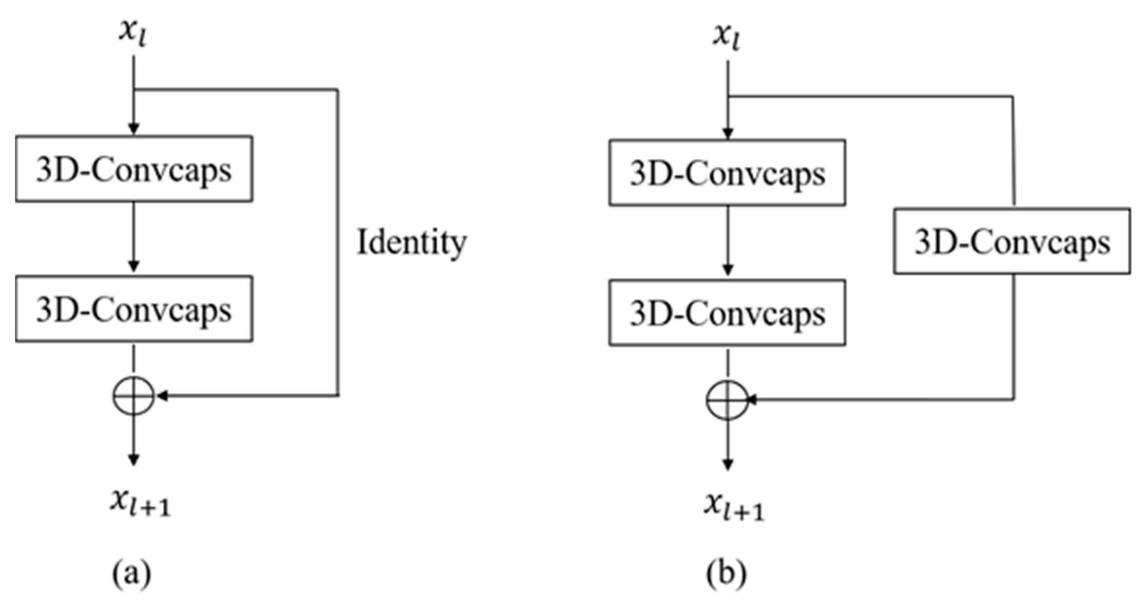
2.1. The Capsule Residual Block

CapsNet has shown more powerful performance than CNN in the HSI classification field with a simple architecture. Typically, the dynamic routing technique, the core of CapsNet that replaced the max-pooling operation, can capture the spatial relationship between different features including the spectral, spatial, and spectral-spatial features. Thus, it can help CapsNet significantly improve the recognized accuracy of the complex geographical objects and usually provide a better classification result with limited labeled samples than CNN-based models. The process of dynamic routing can be represented as

$$s_j=\mathit{G}\left({\displaystyle \sum }_i{\mathit{c}}_{ij}{\widehat{u}}_{j|i}\right)$$

(1)

$${\widehat{u}}_{j|i}=W_{ij}{u}_i$$

(2)

where $s_j$ is the vector output of capsule j, $u_i$ is the output of capsule i, ${\widehat{u}}_{j|i}$ is the prediction vector of $u_i$, $W_{ij}$ is the transform matrix, $c_{ij}$ are coupling coefficients determined by the iterative routing process, and G is the activation function, named Squash [41], to ensure the length of the $s_j$ is between 0 and 1. In this process, the capsule can effectively capture the part-whole relationships of the geographic object.

However, the adjacent capsule layers are fully connected to each other for information transfer in CapsNet, which results in more parameters and computations and easily leads to overfitting when the number of training samples is too small. The 3D-ConvCaps layer implements local routing by combining the 3D convolutional operation with dynamic routing, greatly reducing the number of parameters and mitigating the risk of overfitting. The 3D-ConvCaps layer encapsulates the child capsules into groups, named capsule tensor, during the routing process and uses several adjacent groups of capsules to generate a parent capsule. Thus, the model can focus on more detailed spectral-spatial information during the information transfer process and generate a more robust parent capsule. The process of 3D-ConvCaps layer can be represented as

$${\Phi }^{\mathit{l}+1}=\mathit{G}\left({\displaystyle \sum }_{\mathit{s}}{K}_{\mathit{s}}\cdot U_{\mathit{s}}\right)$$

(3)

$$U=Conv3D\left({\Phi }^{\mathit{l}}\right)$$

(4)

where ${\Phi }^l$ and ${\Phi }^{l+1}$ denote the output of capsule layer l and l + 1, respectively. $U$ denotes the prediction tensor and $U_{\mathit{s}}$ denotes the prediction tensor of capsule tensor s. $K_{\mathit{s}}$ represents the coupling coefficients corresponding to capsule tensor s and determined by the iterative routing process.

Inspired by the success achieved by the CNN-based methods and DC-CapsNet by going deeper and the fact that the deep features are generally more discriminative than shallow features, we want to implement a deeper CapsNet to further explore the potential of CapsNet in the HSI classification field. For the CNN-based methods for HSI classification, residual connections are usually used to capture more discriminative deep spectral-spatial features without excessively increasing the number of trainable parameters. In practice, these connections could enhance the depth of the network, strengthen the flow of information in the network, make the network easier to optimize, and effectively improve the final classification accuracy. Therefore, this paper proposes two kinds of CapsRES blocks based on the 3D-ConvCaps layer and residual connections (Figure 2) to obtain a deeper CapsNet for HSI classification with limited training samples. CapsRES_A is used when the spatial dimensions, the number of feature maps, and the dimension of the feature maps of the residual block’s input x_l and output x_l+1 are the same. Otherwise, CapsRES_B is used. These two CapsRES blocks help us build a deep capsule network with good HSI classification performance when there are few training samples.

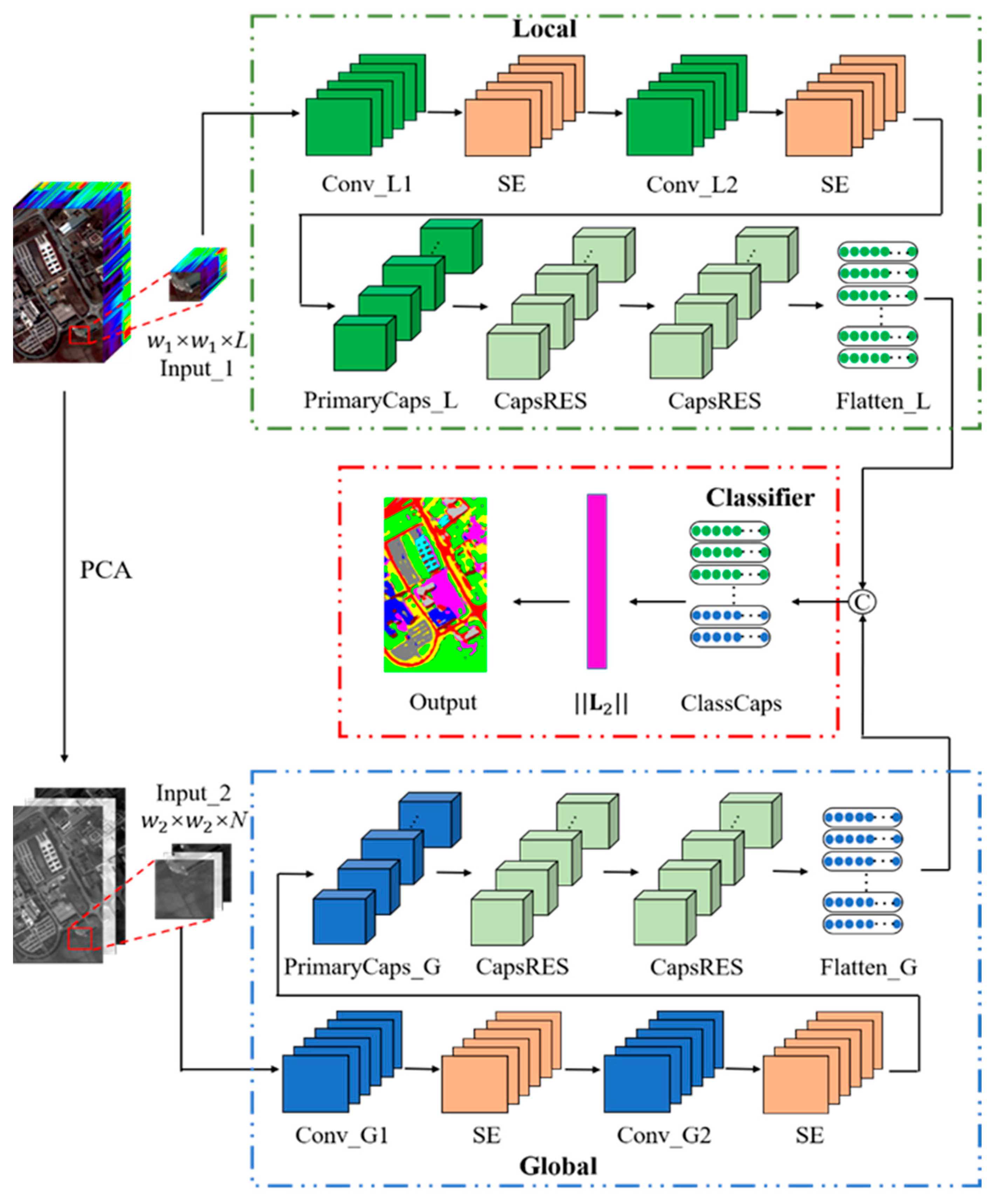
2.2. Local Feature Extraction Module

In this study, the purpose of the local feature extraction module (the top elements in Figure 1) is to extract the spectral and local spatial features from a relatively small sized neighboring pixel block. The input data of the local feature extraction module (Input_1) is a 3D cube from the original HSI with size w1 × w1 × L, that contain both the local spatial information and all spectral information of the original HSI. Different from previous methods based on spectral information that only extract features from the spectral domain of HSIs, the introduction of local spatial information can help the MS-CapsNet model learn the correlations between spectral bands, thereby improving the feature extraction ability of the model. Given the complexity of HSIs, we use two traditional convolutional layers (Conv_L1 and Conv_L2) in the shallow layers of the local feature extraction module to transfer the image to obtain more abstract deep spectral-spatial features. It is worth noting that each convolutional layer is followed by an SE block to refine the shallow local spectral-spatial features of MS-CapsNet. Typically, the attention behavior of the SE block enhances the feature extraction ability of the network by emphasizing valid features and suppressing invalid features for current tasks, which is beneficial for the capsule layer to further explore the spatial relationship between spectral-spatial features. The third layer, PrimaryCaps (PrimaryCaps_L), is the first capsule layer, which converts neurons into capsules. Next, two contiguous CapsRES blocks are used to obtain more robust high-level capsules. Finally, the output of the CapsRES blocks is flattened to the same dimensions to prepare for feature fusion. Furthermore, considering Input_1 is a relatively small sized neighboring pixel block, the method of padding two shallow convolutional layers and PrimaryCaps_L is set to “same”, which can enable the spatial shape of the input and output, to reserve the boundary information and retain more local spatial information.

2.3. Global Feature Extraction Module

The global feature extraction module (the bottom elements in Figure 1) in this paper is mainly responsible for extracting the global spatial information from the input HSI data. The input data of the global feature extraction module (Input_2) are different from those of the local feature extraction module. In practice, PCA is used to reduce the dimensionality of the original HSI data by retaining only a few principal components. Then, a relatively large sized neighboring pixel block with the target pixel as the center, mainly containing the global spatial information of the geographic object, is used as the input data. In practice, the shape of Input_2 can be expressed as w2 × w2 × N. Generally, the number of dynamic routing iterations can seriously affect the calculation speed of the MS-CapsNet model. Thus, we chose a similar model structure to the local feature extraction module but with different parameters for the global feature extraction module; that is, the network is composed of two traditional convolution layers (Conv_G1 and Conv_G2), two SE modules, one PrimaryCaps (PrimaryCaps_G), and two consecutive CapsRES blocks to balance the computational efficiency and classification accuracy for HSIs. It is worth mentioning that a large convolutional kernel is used in the traditional convolution layers and PrimaryCaps of the global feature extraction module to extract the global spatial information. The relatively large size of the neighboring pixel block and convolutional kernel help the global feature extraction module extract more relevant global spatial features in the shallow layer and transport them to the subsequent capsule layers to deeply mine the spatial relationships and patterns that are important for the recognition of complex geographic objects and further improving the classification accuracy with the HSI data. Moreover, due to Input_2 having a large spatial size, the method of padding two shallow convolutional layers and PrimaryCaps_G is set to “valid”, which can reduce the time for training by losing the boundary information.

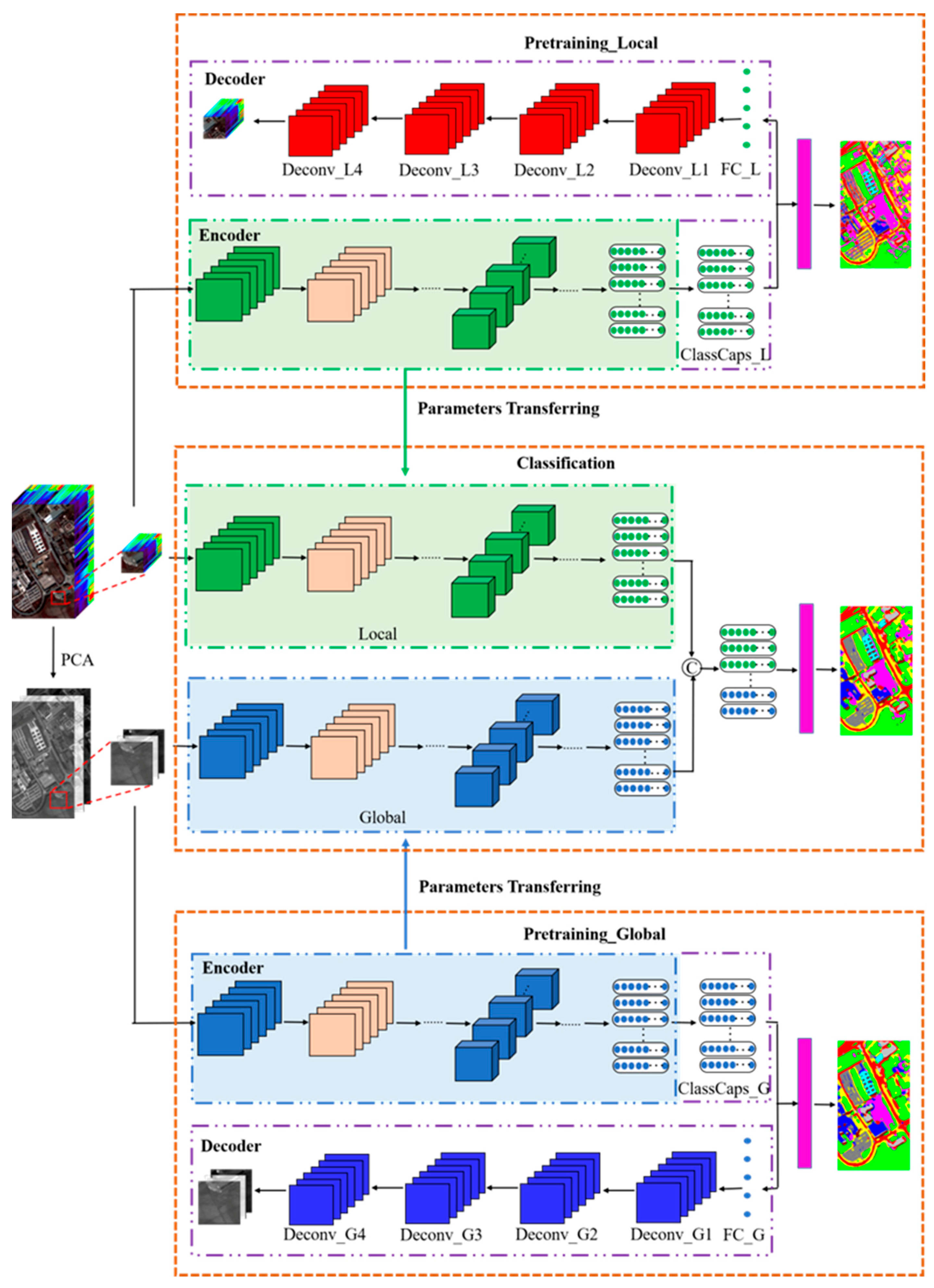
2.4. Framework of the Proposed Model

As shown in Figure 1, the overall framework of MS-CapsNet is composed of the local feature extraction module (Local) and the global feature extraction module (Global). The local feature extraction module is mainly responsible for extracting spectral features and local spatial features from the original HSI data. Its input data are a small portion of adjacent pixel blocks that contains the spectral information of all pixels in the local region. This branch uses a small convolutional kernel for local feature extraction. The global feature extraction module extracts global spatial features from HSIs with only a few principal components after dimensionality reduction. Its input data are adjacent pixel blocks with a relatively large spatial size. To capture global information in the shallow layer of the network, a large convolutional kernel is used for feature extraction. Finally, the local features and global features extracted by the two branches are aggregated using concatenation to predict the final classification result. Therefore, MS-CapsNet can simultaneously extract spectral features, local spatial features and global spatial features and capture the relationship between these features, which can effectively improve the classification performance and alleviate the overfitting problem under conditions of limited training samples in HSI classification.

The main architecture of MS-CapsNet for HSI classification is shown in

Table 1. Architecture of the MS-CapsNet framework.

Layer	Kernel Size	Stride	Batch Normalization	Padding	Activation Function	SE
Local Feature Extraction Module
L1	(1 × 1) × 128	(1, 1)	YES	YES	Mish [57]	YES
L2	(3 × 3) × 64	(1, 1)	YES	YES	Mish	YES
L3	(3 × 3) × 4 × 8	(2, 2)	YES	YES	Mish, Squash	NO
L4-L5	(3 × 3 × 4) × 4 × 8	(1, 1, 4)	NO	YES	Squash	NO
L6-L8	(3 × 3 × 4) × 8 × 8 (3 × 3 × 8) × 8 × 8	(2, 2, 4) (1, 1, 8)	NO	YES	Squash	NO
Global Feature Extraction Module
L1	(5 × 5) × 128	(1, 1)	YES	NO	Mish	YES
L2	(5 × 5) × 64	(1, 1)	YES	NO	Mish	YES
L3	(9 × 9) × 4 × 8	(2, 2)	YES	NO	Mish, Squash	NO
L4-L5	(3 × 3 × 4) × 4 × 8	(1, 1, 4)	NO	YES	Squash	NO
L6-L8	(3 × 3 × 4) × 8 × 8 (3 × 3 × 8) × 8 × 8	(2, 2, 4) (1, 1, 8)	NO	YES	Squash	NO
Feature Fusion Module
Layer	Output size				Activation function
L1	$n_{class}$× 16				Squash

. In the local feature extraction module, the first two layers use 1 × 1 (128 filters) and 3 × 3 (64 filters) convolutional kernels to extract the low-level local spectral-spatial features from the input HSI data. In practice, each convolutional layer is followed by an SE block. The third layer is PrimaryCaps, which adopts a 3 × 3 kernel size to generate a total of 8 feature channels, each of which contains 4 feature maps. Then, there are two consecutive CapsRES blocks. The first block is CapsRES_A, which uses two 3D-ConvCaps layers with 3 × 3 × 4 kernels to output eight 4D convolutional capsule units. The second block is CapsRES_B, which contains three 3D convolutional layers. The first 3D convolution capsule layer of the network backbone and the 3D convolution capsule layer of the residual mapping branch output eight 8D convolutional capsule units through 3 × 3 × 4 kernels, while the second 3D convolution capsule layer of the network backbone uses a 3 × 3 × 8 kernel to generate eight 8D convolution capsule units. The global feature extraction module is similar to the local feature extraction module in structure. It starts with two 5 × 5 convolution layers (128 and 64 filters), both of which is followed by an SE block. The third PrimaryCaps layer uses a 9 × 9 kernel to output 8 feature channels, each with a dimension of 4. Next are two contiguous capsule residual blocks, CapsRES_A and CapsRES_B, with the same parameter settings as in the local feature extraction module. Compared with the local feature extraction module, the global feature extraction module has a larger input data space size and richer spatial information, so we set the padding as “valid” in the two traditional convolutional layers and PrimaryCaps to reduce the computational cost and accelerate the training process. Finally, the outputs of the local feature extraction module and the global feature extraction module are stretched to 32 8D capsules and 72 8D capsules, respectively. After feature fusion, 104 8D capsules containing local and global spectral-spatial features are imported into a fully connected capsule layer, ClassCaps, to obtain the final HSI classification results. Typically, ClassCaps contains n_class (the number of classes) capsules, each of which outputs a 16D vector to represent the corresponding ground object.

2.5. Initialization Strategy

In this paper, the primary components of MS-CapsNet are a global feature extraction module and a local feature extraction module. The local spatial information and spectral information are extracted by the local feature extraction module, and the global feature extraction module is responsible for extracting the global spatial information from HSIs. To obtain more robust local and global spectral-spatial features, two well-designed pretrained deep convolutional capsule networks are further trained to separately extract local and global spectral-spatial information. In practice, inspired by [54], we propose two light decoder networks composed of deconvolutional layers to further improve the feature extraction ability of the pretrained deep convolution capsule networks. The main architecture of the detailed decoder network for the pretrained models is shown in

Table 2. Architecture of the decoder network for the pretrained models.

Local Feature Extraction Module
Fully connected layer
Layer	Number of Neurons		Batch Normalization	Activation Function
L1	3 × 3 × 16		YES	ReLU
Deconvolutional layers
Layer	Kernel Size	Stride	Batch Normalization	Activation Function
L2	(3 × 3) × 64	(1, 1)	NO	ReLU
L3	(3 × 3) × 32	(1, 1)	NO	ReLU
L4	(3 × 3) × 16	(1, 1)	NO	ReLU
L5	(1 × 1) × L	(1, 1)	NO	ReLU
Global feature extraction module
Fully connected layer
Layer	Number of Neurons		Batch Normalization	Activation Function
L1	7 × 7 × 16		YES	ReLU
Deconvolutional Layers
Layer	Kernel Size	Stride	Batch Normalization	Activation Function
L2	(3 × 3) × 64	(1, 1)	NO	ReLU
L3	(5 × 5) × 32	(1, 1)	NO	ReLU
L4	(5 × 5) × 16	(2, 2)	NO	ReLU
L5	(3 × 3) × N	(1, 1)	NO	ReLU

. Then, we transfer all the optimal weight parameters of the two models before the classifier to the local feature extraction module and global feature extraction module of MS-CapsNet to initialize the weight parameters to help the model extract more expressive spectral features, local spatial features, and global spatial features before feature aggregation. Finally, we obtain MS-CapsNet-WI, an extension of MS-CapsNet with well-initialized weight parameters, by fine-tuning the trainable parameters. The workflow of MS-CapsNet-WI for HSI classification is illustrated in Figure 3.

3. Experimental Results and Analysis

To evaluate the performance of MS-CapsNet and MS-CapsNet-WI in HSI classification, four public HSI datasets are introduced in this paper, i.e., Kennedy Space Center (KSC), Pavia University (UP), Salinas (SA), and WHU-Hi-LongKou (LK) [58]. To increase the training speed and avoid the risk of overfitting risk with limited training samples, early stopping and a dynamic learning rate are introduced for MS-CapsNet. Under these conditions, the training process stops if the validation loss does not decrease for 50 epochs, and the learning rate is reduced by half if the validation loss does not decrease for 10 epochs. The maximum number of epochs is set to 200, and the initial learning rate is 0.001. For MS-CapsNet-WI, we use the same early stopping mechanism as MS-CapsNet but not the dynamic learning rate, and the learning rate is set to 0.0001 after the experiments. During the test, we use the overall accuracy (OA), average accuracy (AA), and kappa coefficient (K) to quantitatively appraise the classification performance of the proposed models.

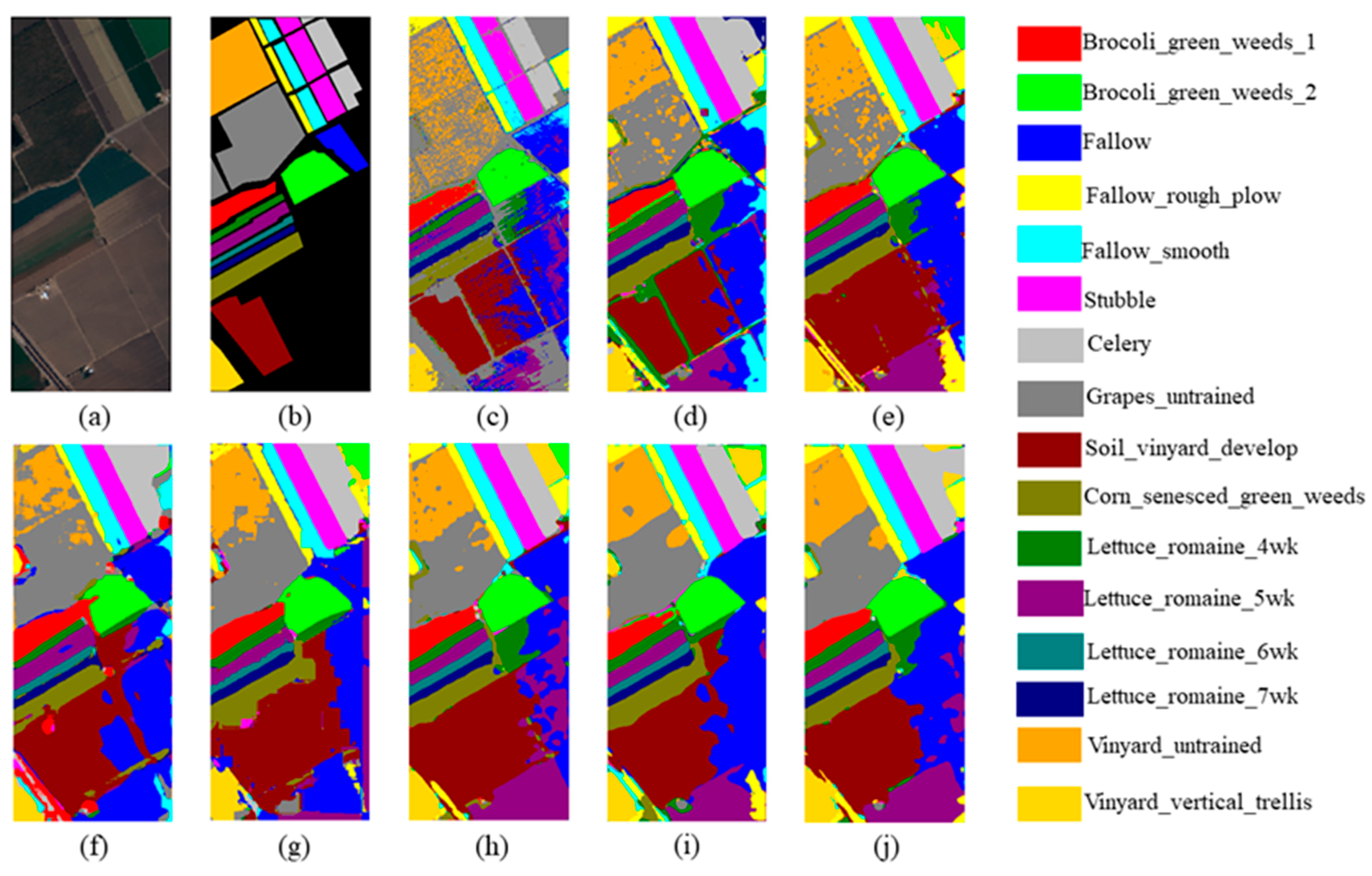
3.1. Experimental Datasets

The KSC dataset, which consists of images of 512 × 614 pixels and 176 bands and includes 13 types of ground objects, was obtained in Florida in 1996. The UP dataset was collected in Pavia, northern Italy. It consists of 103 bands with 610 × 340 pixels images and 9 ground-truth classes. The SA dataset was gathered over Salinas Valley, California. It has images of size 512 × 217 pixels and 204 bands, and 16 different land-cover classes are included. The LK dataset was acquired in Longkou Town, Hubei province, China in 2018. It contains 550 × 400 pixels images with 270 effective bands and nine land-cover classes.

3.2. Influence of Parameters

In this paper, the input data of MS-CapsNet are a set of neighboring pixel blocks separated from the original HSI image. The larger the spatial size of the pixel block, the more spatial-spectral information the model will extract. Therefore, the size of the neighboring pixel block will influence the final classification result of MS-CapsNet. Moreover, the input of the global feature extraction module is the HSI following dimension reduction using PCA. The spatial information contained in the input data is related to the number of principal components; thus, it is an important factor for MS-CapsNet. Furthermore, the depth of the MS-CapsNet model generally has a great impact on its feature extraction ability. Deeper spectral-spatial features tend to be more discriminant, but when the model depth is too large, the number of model parameters will increase, which can easily cause overfitting when the number of training samples is insufficient. The proposed model combines a local feature extraction module and a global feature extraction module; thus, the ability to extract the spectral, local spatial, and global spatial features is related to the depths of these two modules. So, the number of CapsRES blocks directly affects the depth of the model, and further influence the classification performance of the model. Below, we analyze these factors on the four HSI datasets to select the optimal network settings for MS-CapsNet. In addition, the influence of the SE block and the feature aggregation are also explored in this paper.

For all experiments in this section, 5% of the KSC datasets, 1% of the UP and SA datasets, and 0.2% of the LK dataset are used for the training and validation sets, and the remaining labeled samples are used as test samples to evaluate the performance of the MS-CapsNet model.

3.2.1. Neighboring Pixel Block Size

In this section, we discuss the classification performance with different neighboring pixel block sizes in the local feature extraction module and the global feature extraction module. The numbers of principal components and CapsRES blocks in the two branches are set to 3 and 2, respectively. The classification result as shown in

Table 3. Overall accuracy (%) for different spatial sizes of neighboring pixel blocks with the Kennedy Space Center, Pavia University, Salinas, and WHU-Hi-LongKou datasets.

Dataset	Local				Global
	3 × 3	5 × 5	7 × 7	9 × 9	23 × 23	25 × 25	27 × 27	29 × 29
KSC	98.63	98.61	99.27	98.72	98.33	98.10	99.27	97.86
UP	97.83	97.97	98.94	98.83	98.35	98.55	98.94	98.42
SA	96.74	97.31	98.58	98.65	98.05	97.92	98.58	98.61
LK	98.26	98.35	98.47	98.14	98.36	98.43	98.47	97.58

, the global block size is set to 27 × 27 when the OA varies as local block size varies, and the local block size is set to 7 × 7 when the global block size is discussed. It is obvious that OA generally increases as the spatial size of neighboring pixel blocks increases, and a significant threshold effect is observed. However, slight fluctuations are observed when neighboring pixel block size is set to 5 × 5 and 25 × 25 for the KSC dataset and to 25 × 25 for the SA dataset, but the overall trend does not change. For the local branch, the highest OA is obtained when the neighboring pixel block size was 7 × 7 for the KSC, UP, and LK datasets, with a slight increase in the classification performance when we choose a neighboring pixel size of 9 × 9 on the SA dataset. For the global branch, MS-CapsNet achieves the best results with the KSC, UP, and LK datasets when the neighboring pixel size is 27 × 27. In general, pixel blocks with large spatial sizes contain more global spatial information, but more irrelevant information can also be introduced, which poses certain obstacles to the classification performance of the model. Therefore, the OA decreases when the size of the pixel block is set to 29 × 29. For the SA dataset, we observe a similar situation as with the local branch; that is, the OA is the highest when the largest spatial size is chosen for the neighboring pixel blocks. This may be related to the geography types and sample distribution of the HSI dataset. Overall, we believe that setting the spatial size of the input cube to 7 × 7 and 27 × 27 for the local and global feature extraction modules, respectively, may be a good choice for MS-CapsNet.

3.2.2. Number of Principal Components

In this section, we explore the performance of the MS-CapsNet model by setting the number of principal components to 1, 3, 5, 7, and 10. The number of CapsRES blocks in two branches is set to 2, and the spatial sizes of the neighboring pixel blocks are 7 × 7 and 27 × 27 for the local and global feature extraction modules. The classification results as shown in

Table 4. Overall accuracy (%) for different numbers of principal components with the Kennedy Space Center, Pavia University, Salinas, and WHU-Hi-LongKou datasets.

Dataset	1	3	5	7	10
KSC	98.31	99.27	99.02	99.44	99.11
UP	97.85	98.94	99.04	99.19	99.00
SA	97.55	98.58	98.97	98.82	99.04
LK	98.23	98.47	98.54	98.78	98.53

. For the KSC, UP, and LK datasets, the OA increases at first and then decreases with increasing numbers of principal components. The best results, 99.44%, 99.19%, and 98.78%, respectively, are obtained when we choose the first seven principal components. This is because the first few principal components in the HSI dataset generally contain most of the spatial information. An excessive number of principal components will increase the dimensionality of the input data and require more trainable parameters for fitting; therefore, the classification accuracy of MS-CapsNet is reduced. For the SA dataset, the optimal performance is achieved for 9 principal components, but it is only slightly better than the performance for 5 and 7 principal components. Therefore, we choose 7 as the number of principal components for the global feature extraction module of MS-CapsNet. Notably, there is a sudden decline in the OA when the number of principal components for the KSC dataset is 5. This may be related to the large similarity of the spectral-spatial information of certain object classes (e.g., Slash pine, Oak, and Hardwood) in the images for this number of principal com-ponents, leading to misclassification. For the SA dataset, similar fluctuations occur when the number of principal components is 7.

3.2.3. Number of Capsule Residual Blocks

We assess the impact of the number of CapsRES blocks on the HSI classification performance of MS-CapsNet in this section. The spatial sizes of the neighboring pixel blocks for the local and global feature extraction modules are 7 × 7 and 27 × 27, respectively. The number of principal components is set to 7. The classification results are shown in

Table 5. Overall accuracy (%) for different numbers of capsule residual blocks with the Kennedy Space Center, Pavia University, Salinas, and WHU-Hi-LongKou datasets.

Dataset	L1 + G1	L1 + G2	L2 + G1	L2 + G2	L2 + G3	L3 + G3
KSC	99.35	99.48	99.05	99.44	99.34	98.76
UP	99.05	99.17	99.07	99.19	99.30	99.08
SA	98.89	98.40	98.95	98.82	98.44	98.56
LK	98.75	98.67	98.38	98.78	97.86	98.10

. We use L1 + G2 to represent the model with one CapsRES block in the local feature extraction module and two CapsRES blocks in the global feature extraction module. For the KSC dataset, when the number of model layers is relatively small, an increase in the number of CapsRES blocks in the global feature extraction module is often accompanied by an improvement in model classification accuracy, while a decrease in the model accuracy occurs when the number of CapsRES blocks in the local feature extraction module is increased. The model achieves a peak accuracy of 99.44% with the L1 + G2 configuration. The UP dataset contains urban images taken over a university. It contains many ground objects with relatively small areas, such as Painted metal sheets, Asphalt, and Bitumen, as well as classes with a relatively large area, such as Meadows. Therefore, the classification accuracy increases as the number of CapsRES blocks in the two feature extraction modules increases. With this dataset, MS-CapsNet achieves a peak classification accuracy of 99.30% when the CapsRES block configuration is L2 + G3. For the SA dataset, when the model is shallow, the classification accuracy increases as the number of CapsRES blocks in the local feature extraction module increases. For the L2 + G1 CapsRES block configuration, the model has the highest classification accuracy, 98.95%, decreasing as the number of CapsRES blocks in the global feature extraction module increases. This may be related to the type of geography in the SA dataset. Moreover, the model has the highest classification accuracy for the LK dataset, reaching 98.28% when the number of CapsRES blocks in both feature extraction modules is 2. Furthermore, the use of an excessive number of CapsRES blocks will result in overfitting and the classification accuracy will be significantly decreased on all four datasets. Taken together, the use of the L2 + G2 configuration for the number of CapsRES blocks in the two feature extraction modules may be a good choice.

3.2.4. Squeeze-and-Excitation Block

In this section, we discuss the impact of the SE block on the HSI classification performance of MS-CapsNet. The numbers of principal components and CapsRES blocks in the two branches are set to 3 and 2, respectively. The spatial sizes of the neighboring pixel blocks are 7 × 7 for the local feature extraction module and 27 × 27 for the global feature extraction module. The experimental results are shown in

Table 6. Overall accuracy (%) without and with the SE block with the Kennedy Space Center, Pavia University, Salinas, and WHU-Hi-LongKou datasets.

Dataset	NO	YES
KSC	98.87	99.27
UP	98.77	98.94
SA	98.32	98.58
LK	98.33	98.47

. The SE block significantly improves the classification performance of MS-CapsNet with the four HSI datasets. Specifically, the OA of MS-CapsNet with the SE block reached 99.27%, 98.94%, 98.58%, and 98.47% with the KSC, UP, SA, and LK datasets, respectively.

3.2.5. Feature Aggregation

In this section, the influence of feature aggregation is explored. The spatial sizes of the neighboring pixel blocks are 7 × 7 and 27 × 27 for the local and global feature extraction modules, respectively. The number of principal components is 7, and CapsRES block configuration is set to L2 + G2. As shown in

Table 7. Overall accuracy (%) for different feature fusion methods over the Kennedy Space Center, Pavia University, Salinas, and WHU-Hi-LongKou datasets.

Dataset	Local	Global	Local + Global
KSC	97.56	99.14	99.44
UP	97.19	98.48	99.19
SA	96.38	98.57	98.82
LK	97.96	98.31	98.78

, feature aggregation results in higher classification accuracy than use of the local feature extraction module or global feature extraction module alone, achieving OA values of 99.44%, 99.19%, 98.82%, and 98.78% with the KSC, UP, SA, and LK datasets, respectively. This is because the spectral and local spatial features extracted by the local feature extraction module are complementary to the global spatial features extracted by the global feature extraction module. Feature aggregation helps MS-CapsNet exploit the local and global spectral-spatial features more effectively and enhances its generalizability for limited training samples.

3.3. Experimental Results and Discusion

To explore the potential of the model in classifying HSI data, we compare the classification performance of MS-CapsNet and MS-CapsNet-WI with that of SVM [7], 3D-CNN [27], spectral-spatial residual network (SSRN) [30], DFDN [33], nonlocal CapsNet (NLCapsNet) [50], and DC-CapsNet [55] methods with the KSC, IN, UP, and SA datasets. The architecture of MS-CapsNet and MS-CapsNet-WI is set as follows: the neighboring pixel block size is 7 × 7 and 27 × 27 for the local and global feature extraction modules, respectively, the number of principal components is 7, and the capsule residual block configuration is L2 + G2. For all methods, the percentage of training samples and validation samples is set to 3% for the KSC dataset, 0.5% for the UP and SA datasets; and 0.05% for the LK dataset, the remaining labeled samples are used as the test dataset to evaluate the classification performance of the MS-CapsNet model.

Table 8. Classification results from different models with the Kennedy Space Center, Pavia University, Salinas, and WHU-Hi-LongKou datasets.

Dataset	Models	SVM	3D-CNN	SSRN	DFDN	NLCapsNet	DC-CapsNet	MS-CapsNet	MS-CapsNet-WI
KSC	OA (%)	81.83 ± 0.04	87.65 ± 1.89	93.28 ± 1.25	88.43 ± 0.88	93.21 ± 0.79	95.97 ± 1.16	97.67 ± 0.63	98.25 ± 0.66
	AA (%)	73.86 ± 2.33	85.69 ± 2.40	91.62 ± 1.02	87.58 ± 1.44	92.00 ± 0.95	93.43 ± 1.84	96.60 ± 0.71	96.87 ± 1.49
	K × 100	79.73 ± 0.05	86.24 ± 2.11	92.51 ± 1.41	87.11 ± 0.96	92.43 ± 0.88	95.51 ± 1.29	97.41 ± 0.69	98.05 ± 0.73
UP	OA (%)	78.53 ± 0.74	86.55 ± 0.97	95.23 ± 0.57	88.77 ± 1.47	89.79 ± 1.96	96.71 ± 0.38	97.58 ± 0.54	98.41 ± 0.58
	AA (%)	69.94 ± 0.91	82.76 ± 2.07	93.74 ± 0.52	86.06 ± 1.36	87.87 ± 2.05	95.51 ± 0.41	96.71 ± 1.01	97.59 ± 0.81
	K × 100	70.68 ± 0.92	81.96 ± 1.29	93.75 ± 0.77	84.96 ± 2.01	86.42 ± 2.64	95.63 ± 0.50	96.79 ± 0.72	97.89 ± 0.77
SA	OA (%)	83.69 ± 1.39	87.81 ± 1.72	95.29 ± 0.26	88.80 ± 1.78	93.17 ± 1.61	97.14 ± 0.32	97.84 ± 0.74	98.20 ± 0.01
	AA (%)	86.34 ± 2.05	92.18 ± 1.81	97.40 ± 0.13	90.53 ± 2.24	94.69 ± 0.71	98.06 ± 0.43	98.67 ± 0.35	98.60 ± 0.16
	K × 100	81.75 ± 1.57	86.36 ± 1.96	94.76 ± 0.28	87.51 ± 1.99	92.39 ± 1.79	96.82 ± 0.35	97.60 ± 0.82	98.00 ± 0.01
LK	OA (%)	82.89 ± 0.35	92.60 ± 0.88	95.54 ± 0.48	92.54 ± 0.55	92.16 ± 0.91	94.83 ± 0.66	96.99 ± 0.47	97.35 ± 0.45
	AA (%)	45.62 ± 0.52	83.13 ± 1.96	93.75 ± 0.22	80.99 ± 2.17	78.88 ± 1.58	86.56 ± 1.47	93.61 ± 0.44	93.03 ± 1.52
	K × 100	76.45 ± 0.48	90.23 ± 1.12	94.10 ± 0.64	90.15 ± 0.74	89.61 ± 1.20	93.19 ± 0.86	96.03 ± 0.63	96.52 ± 0.60

shows the classification results for all models with the KSC, UP, SA, and LK datasets. The proposed methods achieve the best classification results, with substantially higher accuracies than other outstanding HSI classification methods with the four datasets. The OA reaches 97.67% for MS-CapsNet with the KSC dataset, with improvements of 15.84%, 10.02%, 4.59%, 9.24%, 4.46%, and 1.7% over the SVM, 3D-CNN, SSRN, DFDN, NLCapsNet, and DC-CapsNet methods, respectively. MS-CapsNet-WI further improves the classification accuracy over MS-CapsNet, with OA, AA, and K reaching values of 98.25%, 96.87%, and 0.9805, respectively. For the UP dataset, the highest OA was 97.58% for MS-CapsNet and 98.41% for MS-CapsNet-WI, representing improvements of 0.87% and 1.70% over DC-CapsNet, respectively. With the SA dataset, the best OA is 97.84% for MS-CapsNet and 98.20% for MS-CapsNet-WI, representing 0.70% and 1.06% improvements, respectively, over DC-CapsNet. Similarly, the classification accuracy of the proposed methods is greater than that of the other compared methods with the LK dataset. The OA is 96.99% for MS-CapsNet and 97.35% for MS-CapsNet-WI. Furthermore, the deep learning methods perform much better than SVM with all datasets. The classification accuracy of DC-CapsNet is better than that of the CNN-based methods and NLCapsNet, a shallower model than the 3D-CNN, SSRN, and DFDN models that nevertheless outperforms 3D-CNN and DFDN because of the feature extraction capacity of its capsule layer. Moreover, DFDN seems to overfit due to an excessive number of trainable parameters.

Figure 4, Figure 5, Figure 6 and Figure 7 show the classification maps of the different models for the KSC, UP, SA, and LK datasets. SVM only extracts spectral features in classifying HSI data, so its classification result exhibits much noise. The methods based on spectral-spatial features, including 3D-CNN, SSRN, DFDN, NLCapsNet, and DC-CapsNet, generate better classification maps than SVM. Furthermore, due to the robust nature of the extracted spectral-spatial features, MS-CapsNet and MS-CapsNet-WI achieve more accurate and smoother results that are more similar to the reference false color image than those of the other compared methods. Notably, MS-CapsNet and MS-CapsNet-WI are better than the other models in distinguishing Meadows from Bare Soil in the UP dataset, but the distinction between Bricks and Trees among the unlabeled samples is not ideal. Similar problems also arise with DFDN and NLCapsNet, which introduce global spatial information during the feature extraction stage. This may be because the distribution of label samples of these two classes in the dataset is relatively scattered, and the spatial distance is relatively large. In this instance, the global spatial information could cause some confusion regarding the classification of adjacent Bricks and Trees. In contrast, the methods based on local spectral-spatial features, including 3D-CNN, SSRN, and DC-CapsNet, do not perform well in distinguishing Meadows from Bare Soil, but they have slight advantages in distinguishing certain unlabeled Trees from Bricks in the UP dataset. In future research, we plan to develop an effective scheme for the aggregation of global spatial and local spectral-spatial information.

To further evaluate the generalizability and robustness of the proposed MS-CapsNet and MS-CapsNet-WI, we randomly choose 0.5%, 1%, 3%, 5%, 7%, and 10% of the labeled samples from the KSC, UP, and SA datasets and 0.05%, 0.1%, 0.2%, 0.3%, 0.4%, and 0.5% of the labeled samples from the LK dataset as the training set. Moreover, we introduce one additional dataset, Indian Pines (IN) [54], to provide an additional verification of the robustness of the proposed methods. It contains 145 × 145 pixel images with 200 effective bands and 16 land-cover classes. For IN dataset, the network architecture of MS-CapsNet and MS-CapsNet-WI is the same with the other four datasets, and the number of training samples is the same with the KSC dataset. Figure 8 illustrates the OAs of the SVM, 3D-CNN, SSRN, DFDN, NLCapsNet, DC-CapsNet, MS-CapsNet, and MS-CapsNet-WI methods using these different numbers of training samples. Compared with the deep learning models, the SVM typically has inferior accuracy. Thanks to the light and deep network structure that involves consecutive spectral and spatial residual blocks, the performance of SSRN is better than other CNN-based methods. When the proportion of the training set is less than 3% for the KSC, UP, SA, and IN datasets, the classification results of SSRN are greater than NLCapsNet. For the LK dataset, we choose a much smaller number of training samples than the other four datasets, so the accuracy of SSRN is always higher than NLCapsNet. SSRN even performs better than DC-CapsNet when the ratio of training samples is 0.05% for the LK dataset. Furthermore, DC-CapsNet generally provides better classification results than CNN-based methods and NLCapsNet due to the light network structure and powerful feature extracted ability. Moreover, MS-CapsNet and MS-CapsNet-WI achieve the best classification results among all compared methods with a small number of training samples because of the more discriminative and robust spectral-spatial features that they extract, and MS-CapsNet-WI is better than MS-CapsNet. However, because deep learning models are data-driven methods, their performance is related to the number of training samples. Therefore, the OA of the deep learning models increases rapidly as the number of training samples increases, but the improvements in the proposed methods are not clear. Additionally, the difference in accuracy between the MS-CapsNet and MS-CapsNet-WI is also not obvious while the number of training samples is relatively large.

To study the complexity and computational efficiency of the proposed methods, we also quantitatively discuss the training, test time and parameters of different deep learning models in the following. As shown in

Table 9. Training, test time, and parameters under different models.

Dataset	Methods	3D-CNN	SSRN	DFDN	NLCapsNet	DC-CapsNet	MS-CapsNet	MS-CapsNet-WI
KSC	Train (s)	36.41	60.08	798.56	1492.91	98.40	143.97	269.66
	Test (s)	1.54	5.29	35.49	55.50	2.96	10.01	10.09
	Parameters	2,087,553	309,845	1,244,410	6,068,096	409,728	716,864	-
UP	Train (s)	46.24	67.65	659.64	1441.15	47.42	132.58	307.78
	Test (s)	8.67	11.39	151.76	323.62	20.01	61.77	66.23
	Parameters	832,349	199,153	1,239,922	4,429,696	309,248	654,272	-
SA	Train (s)	61.44	125.94	1562.30	3040.28	129.61	283.18	420.32
	Test (s)	18.86	26.63	373.50	778.01	32.65	87.96	92.87
	Parameters	2,401,756	352,928	1,247,776	7,296,896	454,272	760,384	-
LK	Train (s)	35.29	80.62	2632.34	730.90	57.67	125.84	129.51
	Test (s)	60.41	121.66	6011.48	1633.44	131.30	378.15	329.45
	Parameters	3,497,949	454,129	1,239,922	4,429,696	501,632	675,648	-

, the time costs and parameters of SSRN, DC-CapsNet, MS-CapsNet, and MS-CapsNet-WI are acceptable, and our methods take more computational time and parameters than SSRN and DC-CapsNet. This is because MS-CapsNet and MS-CapsNet-WI are composed of two branches to extract local and global spectral-spatial features and have a deeper network framework, thus, they contain a relatively large number of trainable parameters and need more time to transfer the local and global spectral-spatial features. Fortunately, the classification accuracy of MS-CapsNet and MS-CapsNet-WI is as good as we expect. Moreover, MS-CapsNet-WI uses the elaborated initialization strategy and relatively small learning rate to further improve the final classification accuracy, but small rate usually causes slow convergence speed. Therefore, MS-CapsNet-WI has the same number of parameters as MS-CapsNet but requires more training time. Moreover, the number of parameters for 3D-CNN, DFDN and NLCapsNet is relatively large compared to other deep learning methods. In addition, the computational cost of DFDN and NLCapsNet is higher than other methods, while 3D-CNN takes the least time because of the shallow network structure.

4. Conclusions

In this paper, we proposed a deeper multiscale feature aggregation capsule neural network based on CapsNet for spectral-spatial feature extraction and HSI classification. MS-CapsNet can simultaneously extract the spectral, local spatial, and global spatial features from the input HSI data at different scales through two feature extraction modules. Then, the model aggregates these three kinds of features and outputs the final classification result. Moreover, the SE block is introduced in the shallow layers of the MS-CapsNet to optimize and refine the low-level features and enhance the feature representation ability of the model. Furthermore, two kinds of capsule residual blocks based on residual connections are proposed to build the deep capsule network. Then, we construct the deep network structures of the local feature extraction module and the global feature extraction module to help the model extract more discriminant deep spectral-spatial features. Additionally, an extension of MS-CapsNet based on an elaborate initialization strategy, named MS-CapsNet-WI, is developed to further improve the classification performance with two pretrained deep convolutional capsule networks to find a good set of initializing weight parameters for MS-CapsNet. Experiments with the KSC, UP, SA, and LK datasets show that the proposed methods achieve substantially better performance than state-of-the-art methods in the HSI classification field, even with limited training samples.

Inspired by the potential of MS-CapsNet in performing multiscale feature extraction, we will consider introducing multisource remote sensing images, such as light detection and ranging (LiDAR), synthesis aperture radar (SAR), and multispectral remote sensing images, for classification in the future.

References

1. Gevaert, C.M.; Suomalainen, J.; Tang, J.; Kooistra, L. Generation of Spectral–Temporal Response Surfaces by Combining Multispectral Satellite and Hyperspectral UAV Imagery for Precision Agriculture Applications. IEEE J. Sel. Top. Appl. Earth Observ. Remote Sens. 2015, 8, 3140–3146. [Google Scholar] [CrossRef]
2. Zhang, B.; Wu, D.; Zhang, L.; Jiao, Q.; Li, Q. Application of hyperspectral remote sensing for environment monitoring in mining areas. Environ. Earth Sci. 2012, 65, 649–658. [Google Scholar] [CrossRef]
3. Eslami, M.; Mohammadzadeh, A. Developing a Spectral-Based Strategy for Urban Object Detection from Airborne Hyperspectral TIR and Visible Data. IEEE J. Sel. Top. Appl. Earth Obs. Remote Sens. 2016, 9, 1808–1816. [Google Scholar] [CrossRef]
4. Naoto, Y.; Jonathan, C.; Karl, S. Potential of Resolution-Enhanced Hyperspectral Data for Mineral Mapping Using Simulated EnMAP and Sentinel-2 Images. Remote Sens. 2016, 8, 172. [Google Scholar] [CrossRef] [Green Version]
5. Su, H.; Yu, Y.; Du, Q.; Du, P. Ensemble Learning for Hyperspectral Image Classification Using Tangent Collaborative Representation. IEEE Trans. Geosci. Remote Sens. 2020, 58, 3778–3790. [Google Scholar] [CrossRef]
6. Ham, J.; Chen, Y.; Crawford, M.M.; Ghosh, J. Investigation of the random forest framework for classification of hyperspectral data. IEEE Trans. Geosci. Remote Sens. 2005, 43, 492–501. [Google Scholar] [CrossRef] [Green Version]
7. Melgani, F.; Bruzzone, L. Classification of hyperspectral remote sensing images with support vector machines. IEEE Trans. Geosci. Remote Sens. 2004, 42, 1778–1790. [Google Scholar] [CrossRef] [Green Version]
8. Zhao, Y.; Qian, Y.; Li, C. Improved KNN text classification algorithm with MapReduce implementation. In Proceedings of the 2017 4th International Conference on Systems and Informatics (ICSAI), Hangzhou, China, 11–13 November 2017; pp. 1417–1422. [Google Scholar]
9. Shen, L.; Jia, S. Three-Dimensional Gabor Wavelets for Pixel-Based Hyperspectral Imagery Classification. IEEE Trans. Geosci. Remote Sens. 2011, 49, 5039–5046. [Google Scholar] [CrossRef]
10. Su, H.; Zhao, B.; Du, Q.; Du, P.; Xue, Z. Multifeature dictionary learning for collaborative representation classification of hyperspectral imagery. IEEE Trans. Geosci. Remote Sens. 2018, 56, 2467–2484. [Google Scholar] [CrossRef]
11. Su, H.; Zhao, B.; Du, Q.; Du, P. Kernel collaborative representation with local correlation features for hyperspectral image classification. IEEE Trans. Geosci. Remote Sens. 2019, 57, 1230–1241. [Google Scholar] [CrossRef]
12. Zhao, Y.; Zhang, L.; Kong, S.G. Band-Subset-Based Clustering and Fusion for Hyperspectral Imagery Classification. IEEE Trans. Geosci. Remote Sens. 2011, 49, 747–756. [Google Scholar] [CrossRef]
13. Fauvel, M.; Benediktsson, J.A.; Chanussot, J.; Sveinsson, J.R. Spectral and Spatial Classification of Hyperspectral Data Using SVMs and Morphological Profiles. IEEE Trans. Geosci. Remote Sens. 2008, 46, 3804–3814. [Google Scholar] [CrossRef] [Green Version]
14. Gu, Y.; Chanussot, J.; Jia, X.; Benediktsson, J.A. Multiple Kernel Learning for Hyperspectral Image Classification: A Review. IEEE Trans. Geosci. Remote Sens. 2017, 55, 6547–6565. [Google Scholar] [CrossRef]
15. Hughes, G. On the mean accuracy of statistical pattern recognizers. IEEE Trans. Inf. Theory 1968, 14, 55–63. [Google Scholar] [CrossRef] [Green Version]
16. Chen, Y.; Lin, Z.; Zhao, X.; Wang, G.; Gu, Y. Deep Learning-Based Classification of Hyperspectral Data. IEEE J. Sel. Top. Appl. Earth Observ. Remote Sens. 2014, 7, 2094–2107. [Google Scholar] [CrossRef]
17. Chen, Y.; Zhao, X.; Jia, X. Spectral–Spatial Classification of Hyperspectral Data Based on Deep Belief Network. IEEE J. Sel. Top. Appl. Earth Observ. Remote Sens. 2015, 8, 2381–2392. [Google Scholar] [CrossRef]
18. Mou, L.; Ghamisi, P.; Zhu, X.X. Deep Recurrent Neural Networks for Hyperspectral Image Classification. IEEE Trans. Geosci. Remote Sens. 2017, 55, 3639–3655. [Google Scholar] [CrossRef] [Green Version]
19. Song, W.; Li, S.; Fang, L.; Lu, T. Hyperspectral Image Classification with Deep Feature Fusion Network. IEEE Trans. Geosci. Remote Sens. 2018, 56, 3173–3184. [Google Scholar] [CrossRef]
20. Chen, Y.; Zhu, K.; Zhu, L.; He, X.; Ghamisi, P.; Benediktsson, J.A. Automatic Design of Convolutional Neural Network for Hyperspectral Image Classification. IEEE Trans. Geosci. Remote Sens. 2019, 57, 7048–7066. [Google Scholar] [CrossRef]
21. Liu, B.; Yu, X.; Zhang, P.; Tan, X.; Yu, A.; Xue, Z. A semi-supervised convolutional neural network for hyperspectral image classification. Remote Sens. Lett. 2017, 8, 839–848. [Google Scholar] [CrossRef]
22. Li, W.; Wu, G.; Zhang, F.; Du, Q. Hyperspectral Image Classification Using Deep Pixel-Pair Features. IEEE Trans. Geosci. Remote Sens. 2017, 55, 844–853. [Google Scholar] [CrossRef]
23. Santara, A.; Mani, K.; Hatwar, P.; Singh, A.; Garg, A.; Padia, K.; Mitra, P. BASS Net: Band-Adaptive Spectral-Spatial Feature Learning Neural Network for Hyperspectral Image Classification. IEEE Trans. Geosci. Remote Sens. 2017, 55, 5293–5301. [Google Scholar] [CrossRef] [Green Version]
24. Pan, B.; Shi, Z.; Xu, X. R-VCANet: A New Deep-Learning-Based Hyperspectral Image Classification Method. IEEE J. Sel. Top. Appl. Earth Observ. Remote Sens. 2017, 10, 1975–1986. [Google Scholar] [CrossRef]
25. Chen, Y.; Jiang, H.; Li, C.; Jia, X.; Ghamisi, P. Deep Feature Extraction and Classification of Hyperspectral Images Based on Convolutional Neural Networks. IEEE Trans. Geosci. Remote Sens. 2016, 54, 6232–6251. [Google Scholar] [CrossRef] [Green Version]
26. Li, Y.; Zhang, H.; Shen, Q. Spectral–Spatial Classification of Hyperspectral Imagery with 3D Convolutional Neural Network. Remote Sens. 2017, 9, 67. [Google Scholar] [CrossRef] [Green Version]
27. Srivastava, R.K.; Greff, K.; Schmidhuber, J. Training Very Deep Networks. arXiv 2015, arXiv:1507.06228. [Google Scholar]
28. Paoletti, M.E.; Haut, J.M.; Beltran, R.F.; Plazza, A.J.; Pla, F. Deep pyramidal residual networks for spectral-spatial hyperspectral image classification. IEEE Trans. Geosci. Remote Sens. 2019, 57, 740–754. [Google Scholar] [CrossRef]
29. Zhong, Z.; Li, J.; Luo, Z.; Chapman, M. Spectral–Spatial Residual Network for Hyperspectral Image Classification: A 3-D Deep Learning Framework. IEEE Trans. Geosci. Remote Sens. 2018, 56, 847–858. [Google Scholar] [CrossRef]
30. Zhang, C.; Li, G.; Du, S.; Zhang, X. 3D densely connected convolutional network for hyperspectral remote sensing image classification. Appl. Remote Sens. 2019, 13, 016519. [Google Scholar] [CrossRef]
31. Paoletti, M.E.; Haut, J.M.; Plaza, J.; Plaza, A. Deep&Dense Convolutional Neural Network for Hyperspectral Image Classification. Remote Sens. 2018, 10, 1454. [Google Scholar] [CrossRef] [Green Version]
32. Zhang, C.; Li, G.; Lei, R.; Du, S.; Zhang, X.; Zheng, H.; Wu, Z. Deep Feature Aggregation Network for Hyperspectral Remote Sensing Image Classification. IEEE J. Sel. Top. Appl. Earth Observ. Remote Sens. 2020, 13, 5314–5325. [Google Scholar] [CrossRef]
33. Li, X.; Ding, M.; Pižurica, A. Deep Feature Fusion via Two-Stream Convolutional Neural Network for Hyperspectral Image Classification. IEEE Trans. Geosci. Remote Sens. 2020, 58, 2615–2629. [Google Scholar] [CrossRef] [Green Version]
34. Liu, Y.; Gao, L.; Xiao, C.; Qu, Y.; Zheng, K.; Marinoni, A. Hyperspectral Image Classification Based on a Shuffled Group Convolutional Neural Network with Transfer Learning. Remote Sens. 2020, 12, 1780. [Google Scholar] [CrossRef]
35. Liang, H.; Li, Q. Hyperspectral Imagery Classification Using Sparse Representations of Convolutional Neural Network Features. Remote Sens. 2016, 8, 99. [Google Scholar] [CrossRef] [Green Version]
36. Gong, Z.; Zhong, P.; Yu, Y.; Hu, W.; Li, S. A CNN With Multiscale Convolution and Diversified Metric for Hyperspectral Image Classification. IEEE Trans. Geosci. Remote Sens. 2019, 57, 3599–3618. [Google Scholar] [CrossRef]
37. Lu, Z.; Xu, B.; Sun, L.; Zhan, T.; Tang, S. 3-D Channel and Spatial Attention Based Multiscale Spatial–Spectral Residual Network for Hyperspectral Image Classification. IEEE J. Sel. Top. Appl. Earth Observ. Remote Sens. 2020, 13, 4311–4324. [Google Scholar] [CrossRef]
38. Chen, Y.; Zhu, L.; Ghamisi, P.; Jia, X.; Li, G.; Tang, L. Hyperspectral images classification with Gabor filtering and convolutional neural network. IEEE Geosci. Remote Sens. Lett. 2017, 14, 2355–2359. [Google Scholar] [CrossRef]
39. Zhu, L.; Chen, Y.; Ghamisi, P.; Benediktsson, J.A. Generative Adversarial Networks for Hyperspectral Image Classification. IEEE Trans. Geosci. Remote Sens. 2018, 56, 5046–5063. [Google Scholar] [CrossRef]
40. Zhong, Z.; Li, J.; Clausi, D.A.; Wong, A. Generative Adversarial Networks and Conditional Random Fields for Hyperspectral Image Classification. IEEE Trans. Cybern. 2020, 50, 3318–3329. [Google Scholar] [CrossRef] [Green Version]
41. Sabour, S.; Frosst, N.; Hinton, G. Dynamic routing between capsules. arXiv 2014, arXiv:1710.09829. [Google Scholar]
42. Ma, Y.; Zheng, Z.; Guo, Z.; Mou, F.; Zhou, F.; Kong, R.; Hou, A. Classification Based on Capsule Network with Hyperspectral Image. In Proceedings of the International Geoscience and Remote Sensing Symposium, Yokohama, Japan, 28 July–2 August 2019; pp. 2750–2753. [Google Scholar]
43. Deng, F.; Pu, S.; Chen, X.; Shi, Y.; Yuan, T.; Pu, S. Hyperspectral Image Classification with Capsule Network Using Limited Training Samples. Sensors 2018, 18, 3153. [Google Scholar] [CrossRef] [PubMed] [Green Version]
44. Wang, W.; Li, H.; Pan, L.; Yang, G.; Du, Q. Hyperspectral Image Classification Based on Capsule Network. In Proceedings of the International Geoscience and Remote Sensing Symposium, Valencia, Spain, 22–27 July 2018; pp. 3571–3574. [Google Scholar]
45. Jia, S.; Zhao, B.; Tang, L.; Feng, F.; Wang, W. Spectral–spatial classification of hyperspectral remote sensing image based on capsule network. J. Eng. 2019, 2019, 7352–7355. [Google Scholar] [CrossRef]
46. Paoletti, M.E.; Haut, J.M.; Beltran, R.F.; Plaza, J.; Plaza, A.; Li, J. Capsule Networks for Hyperspectral Image Classification. IEEE Trans. Geosci. Remote Sens. 2019, 57, 2145–2160. [Google Scholar] [CrossRef]
47. Jiang, X.; Liu, W.; Zhang, Y.; Liu, J.; Li, S.; Lin, J. Spectral–Spatial Hyperspectral Image Classification Using Dual-Channel Capsule Networks. IEEE Geosci. Remote Sens. Lett. 2021, 18, 1094–1098. [Google Scholar] [CrossRef]
48. Yin, J.; Li, S.; Zhu, H.; Luo, X. Hyperspectral Image Classification Using CapsNet With Well-Initialized Shallow Layers. IEEE Geosci. Remote Sens. Lett. 2019, 16, 1095–1099. [Google Scholar] [CrossRef]
49. Lei, R.; Zhang, C.; Du, S.; Wang, C.; Zhang, X.; Zheng, H.; Huang, J.; Yu, M. A non-local capsule neural network for hyperspectral remote sensing image classification. Remote Sens. Lett. 2020, 12, 40–49. [Google Scholar] [CrossRef]
50. Li, H.; Wang, W.; Pan, L.; Li, W.; Du, Q.; Tao, R. Robust Capsule Network Based on Maximum Correntropy Criterion for Hyperspectral Image Classification. IEEE J. Sel. Top. Appl. Earth Observ. Remote Sens. 2020, 13, 738–751. [Google Scholar] [CrossRef]
51. Wang, W.-Y.; Li, H.-C.; Deng, Y.-J.; Shao, L.-Y.; Lu, X.-Q.; Du, Q. Generative Adversarial Capsule Network with ConvLSTM for Hyperspectral Image Classification. IEEE Geosci. Remote Sens. Lett. 2021, 18, 523–527. [Google Scholar] [CrossRef]
52. Zhang, H.; Meng, L.; Wei, X.; Tang, X.; Tang, X.; Wang, X.; Jin, B.; Yao, W. 1D-Convolutional Capsule Network for Hyperspectral Image Classification. arXiv 2019, arXiv:1903.09834. [Google Scholar]
53. Zhu, K.; Chen, Y.; Ghamisi, P.; Jia, X.; Benediktsson, J.A. Deep Convolutional Capsule Network for Hyperspectral Image Spectral and Spectral-Spatial Classification. Remote Sens. 2019, 11, 582. [Google Scholar] [CrossRef] [Green Version]
54. Lei, R.; Zhang, C.; Liu, W.; Zhang, L.; Zhang, X.; Yang, Y.; Huang, J.; Li, Z.; Zhou, Z. Hyperspectral Remote Sensing Image Classification Using Deep Convolutional Capsule Network. IEEE J. Sel. Top. Appl. Earth Observ. Remote Sens. 2021, 14, 8297–8315. [Google Scholar] [CrossRef]
55. He, K.; Zhang, X.; Ren, S.; Sun, J. Deep residual learning for image recognition. arXiv 2015, arXiv:1512.03385. [Google Scholar]
56. Hu, J.; Shen, L.; Sun, G. Squeeze-and-excitation networks. In Proceedings of the IEEE Conference on Computer Vision and Pattern Recognition (CVPR), Salt Lake City, UT, USA, 18–23 June 2018; pp. 7132–7141. [Google Scholar]
57. Misra, D. Mish: A Self Regularized Non-Monotonic Neural Activation Function. arXiv 2019, arXiv:1908.08681. [Google Scholar]
58. Zhong, Y.; Hu, X.; Luo, C.; Wang, X.; Zhao, J.; Zhang, L. WHU-Hi: UAV-borne hyperspectral with high spatial resolution (H2) benchmark datasets and classifier for precise crop identification based on deep convolutional neural network with CRF. Remote Sens. Environ. 2020, 250, 112012. [Google Scholar] [CrossRef]
Figure 1. Over framework of the MS-CapsNet. Input_1 and Input_2 denote the input data of the local feature extraction module (Local) and global feature extraction module (Global), respectively. w1 is the spatial size of Input_1 and w2 is the spatial size of Input_2. L represents the number of spectral dimensions of the input data. N denotes the number of principal components of the input HSI data after dimension reduction using principal component analysis (PCA). ‖L2 ‖ denotes the L2-norm of a vector.
Remotesensing 14 01652 g001
Figure 2. (a) Capsule residual block A, (b) Capsule residual block B.
Remotesensing 14 01652 g002
Figure 3. Workflow of the MS-CapsNet with well-initialized weight parameters for HSI classification.
Remotesensing 14 01652 g003
Figure 4. Classification results for different models with the Kennedy Space Center dataset: (a) false color image, (b) ground-truth labels, and (cj) classification results for SVM, 3D-CNN, SSRN, DFDN, NLCapsNet, DC-CapsNet, MS-CapsNet, and MS-CapsNet-WI.
Remotesensing 14 01652 g004
Figure 5. Classification results for different models with the Pavia University dataset: (a) false color image, (b) ground-truth labels, and (cj) classification results for SVM, 3D-CNN, SSRN, DFDN, NLCapsNet, DC-CapsNet, MS-CapsNet, and MS-CapsNet-WI.
Remotesensing 14 01652 g005
Figure 6. Classification results for different models with the Salinas dataset: (a) false color image, (b) ground-truth labels, and (cj) classification results for SVM, 3D-CNN, SSRN, DFDN, NLCapsNet, DC-CapsNet, MS-CapsNet, and MS-CapsNet-WI.
Remotesensing 14 01652 g006
Figure 7. Classification results for different models with the WHU-Hi-LongKou dataset: (a) false color image, (b) ground-truth labels, and (cj) classification results for SVM, 3D-CNN, SSRN, DFDN, NLCapsNet, DC-CapsNet, MS-CapsNet, and MS-CapsNet-WI.
Remotesensing 14 01652 g007
Figure 8. Overall accuracy of different models with different training set sizes: (a) Kennedy Space Center, (b) Pavia University, (c) Salinas, (d) WHU-Hi-LongKou, and (e) Indian Pines.
Remotesensing 14 01652 g008