Article

Applying Machine Learning and Time-Series Analysis on Sentinel-1A SAR/InSAR for Characterizing Arctic Tundra Hydro-Ecological Conditions

1
Department of Geography, Environment and Geomatics, University of Guelph, Guelph, ON N1G 2W1, Canada
2
The Canada Center for Mapping and Earth Observation, Ottawa, ON K1S 5K2, Canada
*
Author to whom correspondence should be addressed.
Remote Sens. 2022, 14(5), 1123; https://doi.org/10.3390/rs14051123
Submission received: 25 January 2022 / Revised: 22 February 2022 / Accepted: 22 February 2022 / Published: 24 February 2022
(This article belongs to the Special Issue Remote Sensing of Polar Regions)

Abstract

:
Synthetic aperture radar (SAR) is a widely used tool for Earth observation activities. It is particularly effective during times of persistent cloud cover, low light conditions, or where in situ measurements are challenging. The intensity measured by a polarimetric SAR has proven effective for characterizing Arctic tundra landscapes due to the unique backscattering signatures associated with different cover types. However, recently, there has been increased interest in exploiting novel interferometric SAR (InSAR) techniques that rely on both the amplitude and absolute phase of a pair of acquisitions to produce coherence measurements, although the simultaneous use of both intensity and interferometric coherence in Arctic tundra image classification has not been widely tested. In this study, a time series of dual-polarimetric (VV, VH) Sentinel-1 SAR/InSAR data collected over one growing season, in addition to a digital elevation model (DEM), was used to characterize an Arctic tundra study site spanning a hydrologically dynamic coastal delta, open tundra, and high topographic relief from mountainous terrain. SAR intensity and coherence patterns based on repeat-pass interferometry were analyzed in terms of ecological structure (i.e., graminoid, or woody) and hydrology (i.e., wet, or dry) using machine learning methods. Six hydro-ecological cover types were delineated using time-series statistical descriptors (i.e., mean, standard deviation, etc.) as model inputs. Model evaluations indicated SAR intensity to have better predictive power than coherence, especially for wet landcover classes due to temporal decorrelation. However, accuracies improved when both intensity and coherence were used, highlighting the complementarity of these two measures. Combining time-series SAR/InSAR data with terrain derivatives resulted in the highest per-class F1 score values, ranging from 0.682 to 0.955. The developed methodology is independent of atmospheric conditions (i.e., cloud cover or sunlight) as it does not rely on optical information, and thus can be regularly updated over forthcoming seasons or annually to support ecosystem monitoring.

1. Introduction

The Arctic tundra biome is among the most vulnerable landscapes on Earth, undergoing dramatic changes to vegetation, water, and soil surface properties over recent decades. These widespread physical ecosystem changes are driven by rising concentrations of greenhouse gases [1], resulting in fundamental consequences to wildlife [2] and human populations [3]. Despite being one of the coldest biomes on Earth, this water-rich region is warming twice as fast as the global average—a phenomenon known as arctic amplification [4]. Accelerated warming of the climate is having profound impacts on high-latitude freshwater-terrestrial processes, including permafrost thaw [5], wetland flooding frequency [6], vegetation shifts such as shrub expansion [7], and altered partitioning between groundwater and surface water [8]. Permafrost degradation, or active layer thickening, is particularly important because of the role permafrost plays in governing water flow, soil moisture, and storage [9]. The Arctic tundra permafrost contains twice as much carbon as there is in the atmosphere [10], making warming-induced permafrost thaw a concern for immense greenhouse gas emissions that would support a permafrost carbon feedback, further accelerating warming of the Earth [11]. Landcovers with wet or moist surfaces (i.e., wetlands) contain some of the largest stores of soil carbon due to low decomposition rates, making the transient zone between inundated and dry areas very susceptible to increased carbon loss under a shifting climate [12]. Therefore, there is a growing need to map and frequently monitor Arctic tundra ecosystems and their changing conditions.
Arctic tundra regions are remote and often inaccessible environments, making in situ observations and field-based data collection a challenging task. Constraints around weather, low light conditions, and lack of infrastructure make satellite remote sensing the only option for consistent, timely, and repeatable data collection across this spatially extensive biome [13]. Optical satellite sensors (e.g., Landsat) have traditionally been used to develop and validate Arctic tundra landcover products [14]. However, these passive sensors are dependent on the sun’s electromagnetic energy and are affected by atmospheric clouds or haze. Synthetic aperture radar (SAR), in contrast, can operate independently of weather and during day or night, overcoming the limitations of optical remote sensing by providing reliable time-series data. Several recent studies have demonstrated the value of active SAR imaging for classification and mapping of Arctic tundra environments [15,16,17,18,19,20,21].
SAR imaging systems are also appropriate for Arctic tundra ecosystem mapping and monitoring because of the sensitivity of microwaves to dielectric moisture and the physical properties of vegetation [16,22,23]. Yet, until recently, SAR data of high spatial resolution (e.g., < or = 10 m) have not been frequently collected at regional to global scales. The launch of the European Space Agency (ESA) Copernicus Sentinel-1A and -1B satellites in 2014 and 2016 changed this, resulting in SAR observations collected at 10 m spatial resolution and with a temporal revisit time of 12 days for each satellite, or 6 days when combined [24]. This unprecedented source of SAR data has led to remarkable developments in spaceborne remote sensing. Additionally, dense stacks of multi-temporal Sentinel-1 SAR data are permitting the advancement of innovative remote sensing methods, one of which is repeat-pass Interferometric SAR (InSAR [25]).
InSAR, which uses both the phase and amplitude of the backscattered energy, relies on two or more co-registered SAR images to produce measurements called interferograms. Interferogram images contain information associated with differences in the phase of the SAR signal returned to the satellite. Interferometric coherence observations produced from InSAR analysis have been of great interest recently, with studies demonstrating the efficacy of time-series InSAR products over a variety of environments, such as urban [26,27,28], wetland [29,30,31,32,33], permafrost [34,35,36], forested [37,38,39], and ice-covered sea [40,41,42] areas.
Coherence describes the correlation between the SAR signals acquired at two different moments in time and is related to the phase variance. For InSAR to be useful in landcover characterization, coherence must be preserved between image pairs. Coherence preservation implies that a target does not move or change. For distributed targets in natural environments, this can be challenging, especially for longer temporal baselines (i.e., the time between image acquisitions). The amount of phase noise (i.e., decorrelation) is associated with the SAR sensor’s characteristics, including temporal and spatial baselines [43], wavelength (e.g., X-, C-, or L-band [44]), and polarization [45]. Moreover, decorrelation can be caused by changes in physical surface properties, such as soil moisture, vegetation, and water levels [46]. For example, phenological changes to vegetation, or even movement of leaves and branches, may lead to decorrelation.
Despite the promising results and diverse applications of InSAR, there is limited research on this technique’s ability to characterize Arctic tundra ecosystems. Most research employing SAR for mapping high-latitude landcovers have used only backscatter intensity [18,20,21] or decomposition products [15,16,17,19] from a fully polarimetric SAR. Thus, the primary aim of this study was to fill this notable gap in the literature by investigating the potential of both dual-polarimetric SAR intensity and coherence products for the characterization of highly transient Arctic tundra systems. In particular, our study’s objectives were:
  • To analyze the temporal signatures of intensity and coherence measurements from Sentinel-1A C-band SAR data in relation to environmental conditions, thus providing insight on their utility for landcover characterization;
  • To develop a machine learning methodology capable of identifying the hydro-ecological state (e.g., wet or dry, and general vegetation structure) of Arctic tundra landcovers using a time series of SAR/InSAR data and terrain metrics;
  • To provide recommendations on the efficacy of each input data source for the development of baseline landcover data.

2. Materials and Methods
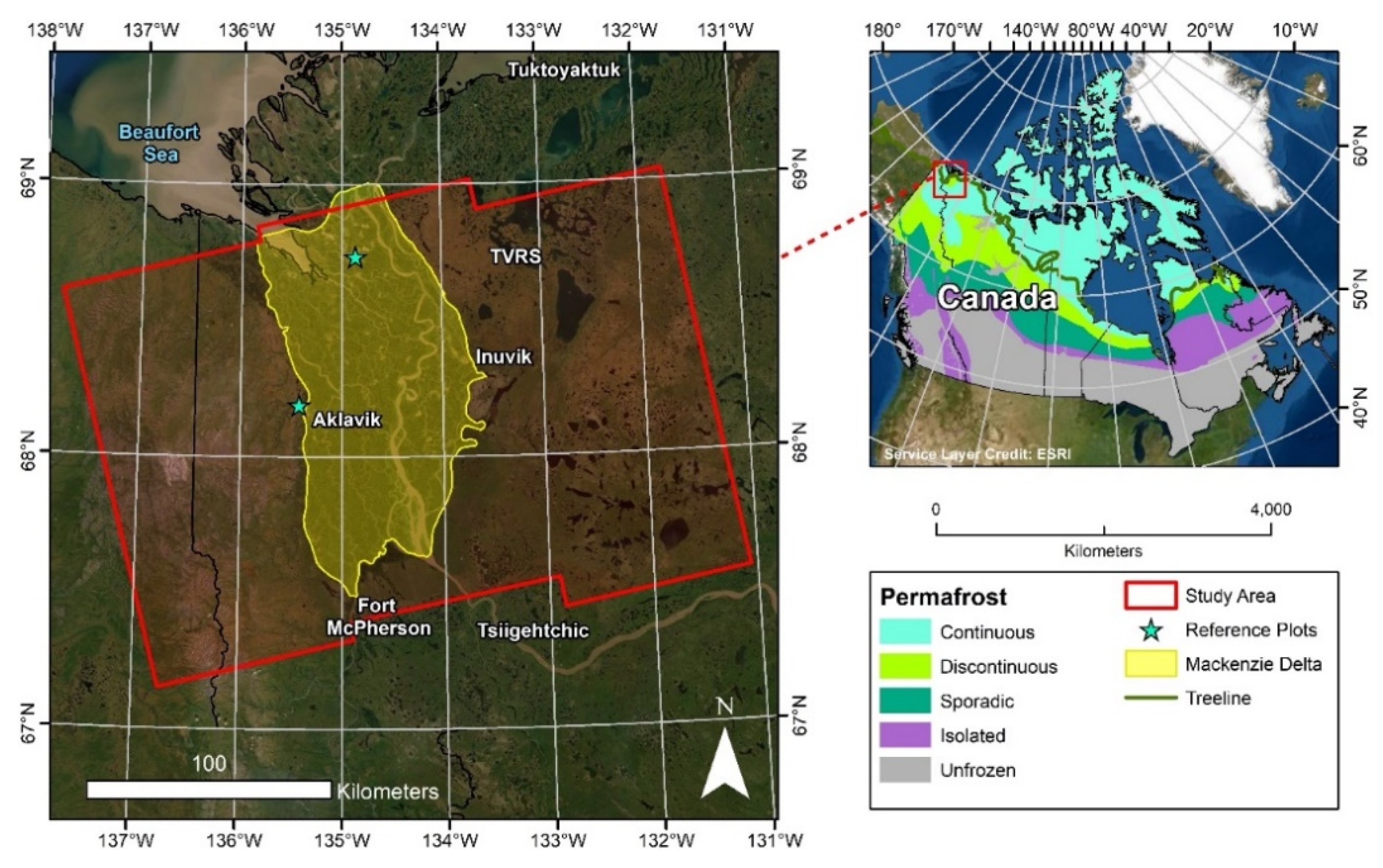
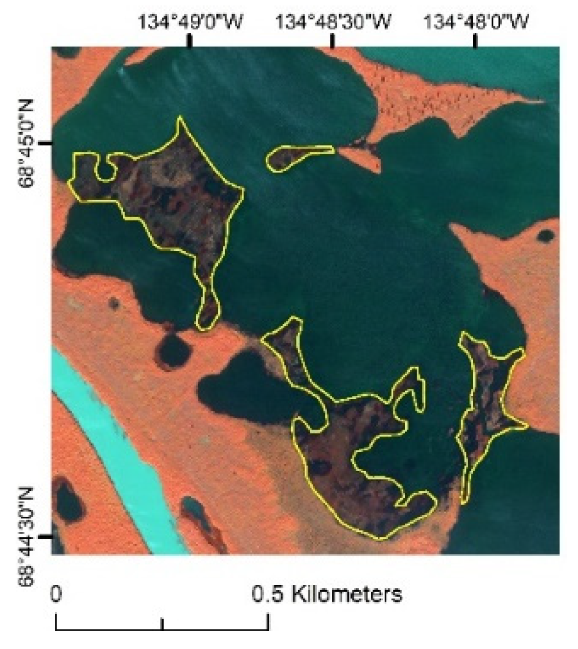
2.1. Study Area

The study area for this mapping experiment was the Mackenzie Delta and surrounding region (Figure 1), as this area represents a variety of Arctic tundra landcovers. The Mackenzie Delta is a post-glacial low-lying alluvial plain located in Canada’s western Arctic, in the Northwest Territories. Inuvik and Aklavik are the principal settlements in the region. For reference, located 50 km north of Inuvik is the Trail Valley Creek Research Station (68°44′25″N 133°29′36″W) which has been a hub for vegetation, permafrost, snow and other land and ecosystem change research [47,48,49]. The delta is part of the Mackenzie River Basin (MRB), which is the second largest river basin in North America, occupying 20% of Canada’s landmass. This area is mainly drained by the Mackenzie River, which is Canada’s longest, flowing northwest out from Great Slave Lake through the delta and into the Beaufort Sea, Arctic Ocean. It is also the largest riverine source of organic carbon and sediment to the Arctic Ocean [50]. Recent studies have shown an increase in discharge in the Mackenzie River, suggesting a northern response to changing climatic conditions [51].
The Mackenzie delta is an incredibly productive, sensitive, and dynamic ecosystem, and is the largest arctic delta in North America with an area of 13,000 km2, and the world’s second largest [52]. The delta provides important habitat for mammals, fish, and migratory birds, which is recognized through the establishment of the Kendall Island Bird Sanctuary. Surrounding the delta to the east are dry, hilly uplands of the Tuktoyaktuk Coastlands consisting of various permafrost features such as polygonal terrain, ice wedges, and pingos. To the west are the Richardson Mountains, part of the northernmost ranges of the Cordillera, which parallel the boundary between the Northwest Territories and the Yukon.
The Mackenzie Delta is considered part of the discontinuous permafrost zone largely due to shifting river channels and the presence of thousands of lakes and wetlands, whereas the surrounding tundra uplands contain ice-rich continuous permafrost [53]. The dynamic hydrology of the delta has shown to result in 95% surface water coverage at flood peak [54], making it an excellent area to assess the efficacy of Earth observation satellite data for hydrological mapping and monitoring. Moreover, peak flooding often occurs following winter ice break up and during the summer after heavy rainfalls [55].

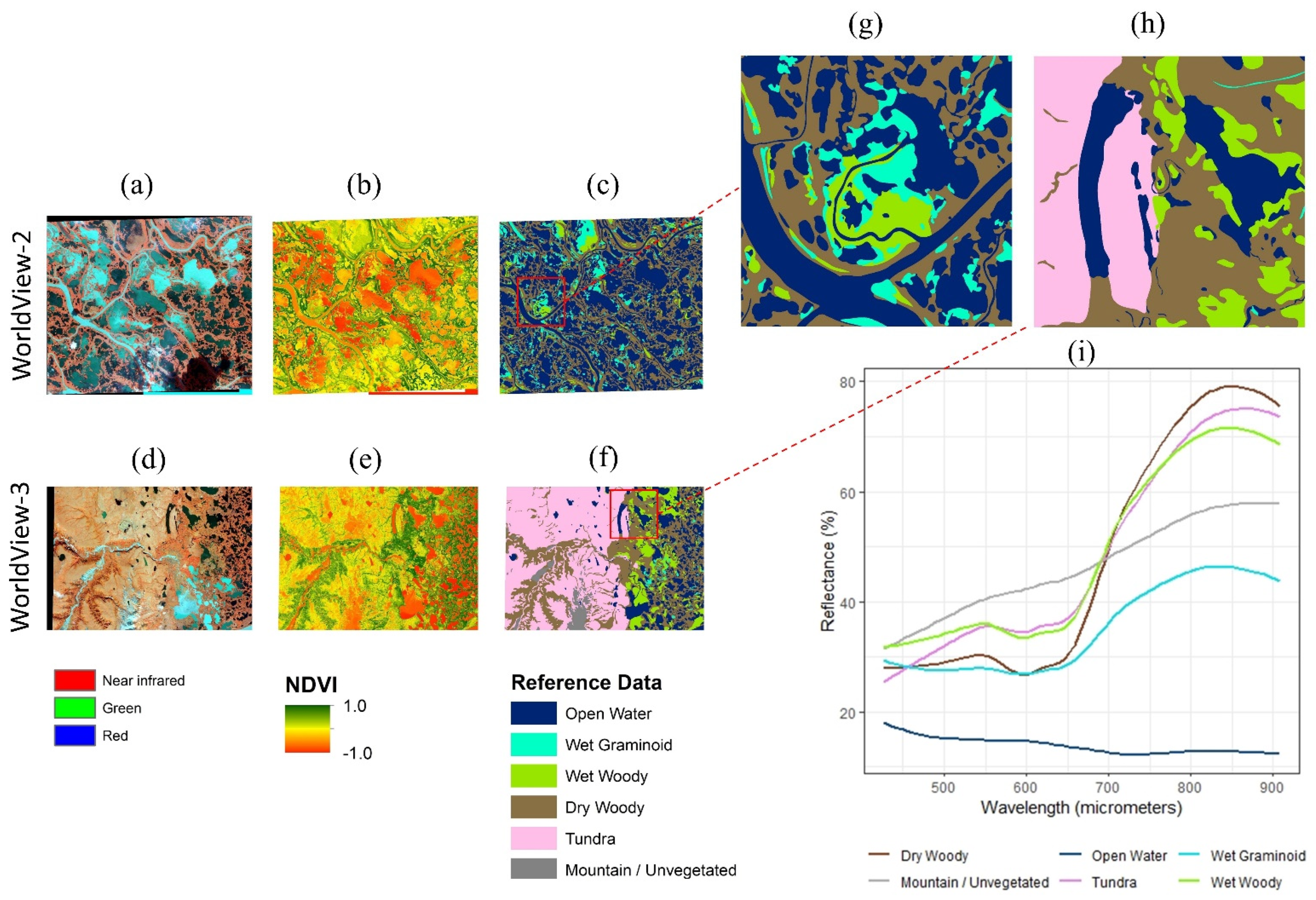
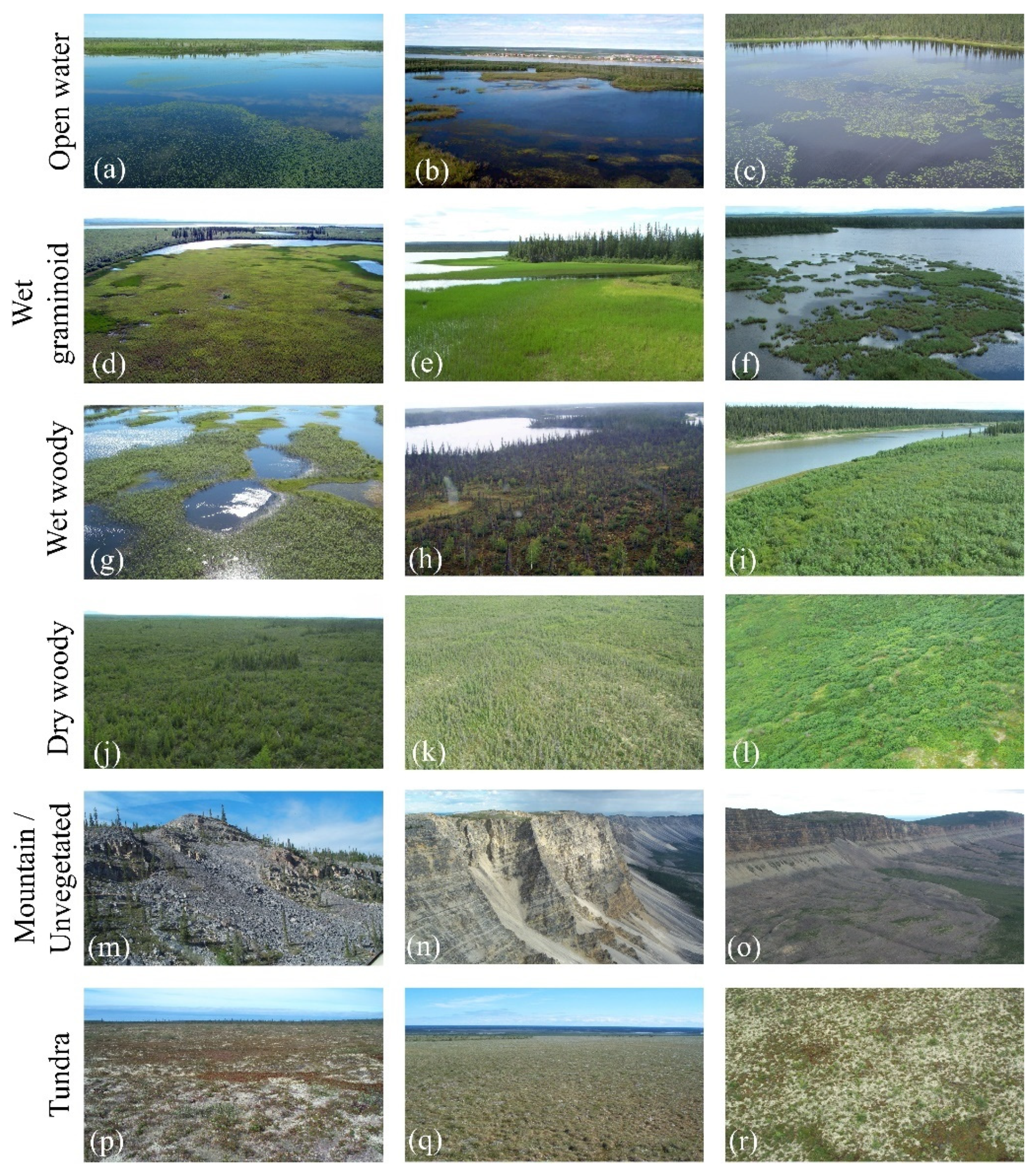
2.2. Vegetation of the Mackenzie Delta and Hydro-Ecological Classes of Interest

The Mackenzie Delta transitions from boreal forest in the south to low-shrub tundra in the north, a result of the region’s climatic gradient and traversing of the treeline. The northern tundra of the delta is dominated by sedges and dwarf shrubs, with specific successional communities influenced by flooding and sedimentation processes [56]. This includes hydrophilic graminoids in poorly drained areas that transition from open water areas, such as sedges (Carex aquatilis) and emergent horsetail (Equisetum). Willow (Salix spp.) and alder (Alnus crispa) species are also very common, found along frequently flooded lakeshores and levees. Dwarf to low ericaceous shrubs commonly grow on the drier uplands. The central and southern parts of the delta more commonly contain dry white spruce (Picea glauca) forests, tall shrub communities, and open canopy peatlands with stunted woody vegetation and wet organic soils (Sphagnum spp.).
For this experiment, we identified six main semantic classes of interest found in the study area, defined based on dominant vegetation composition and/or hydrological properties. Classes were defined with consideration of the major influences on SAR backscatter, including physical vegetation structure and moisture. Classes included open water, wet graminoid, wet woody, dry woody, tundra, and mountain/unvegetated (Figure 2). Open water areas included lakes, ponds, and linear features such as streams and channels, and could contain aquatic plants (e.g., Nuphar spp.). Wet graminoid areas were poorly drained areas that experienced temporally dynamic flooding and drawdown processes and contained sedges and rushes with little presence of shrubs or trees (<20%). The wet woody class was poorly to imperfectly drained areas with wet soils, often visible ponding, and the presence of woody vegetation (>20%). The hydrology of wet woody areas was less dynamic than that of open water and wet graminoid areas, and contained willows, alder, and sometimes an open canopy coverage of standing dead or live spruce species. Woody peatlands were included in this class. Dry woody areas were vegetated uplands with well drained and dry soils, and contained either a very dense coverage of ericaceous shrubs or thick needleleaf or deciduous trees. Tundra areas were elevated regions outside of the delta that were well drained, having continuous permafrost, and mostly contained a coverage of grasses, lichens, and mosses with relatively small areas of trees and shrubs [57]. Mountain/unvegetated areas contained exposed rock or soil with little to no vegetation.

2.3. Reference Data

Spatially referenced training and testing polygons were collected and validated using high-resolution multi-spectral WorldView-2 and -3 satellite imagery (Figure 3). Two scenes were acquired for this task, one located in the low-shrub northern region of the delta (imaged 9 July 2020), and a second in the middle-south region of the delta covering a range of ecotypes, including woody wetlands, exposed mountains, and sparsely vegetated tundra (imaged on 17 August 2020). Both scenes were acquired as 11 bit GeoTIFF raster files with a ground sample distance (GSD) spatial resolution of 1.84 m. Spectral bands spanned the visible to near infrared regions of the electromagnetic spectrum, and included coastal blue (400–450 nanometers; nm), blue (450–510 nm), green (510–580 nm), yellow (585–625 nm), red (630–690 nm), red edge (705–745 nm), near infrared-1 (770–895 nm), and near infrared-2 (860–1040 nm) bands. To assist in the photointerpretation process, a normalized differenced vegetation index (NDVI [58]) layer was derived.
While the high-resolution imagery and NDVI layer were the primary datasets used for digitizing, topographic information from a digital elevation model (DEM) also supported the interpretation process (e.g., for identifying depressions and low-lying areas). DEM characteristics are described later in Section 2.10. Both WorldView-2 and -3 scenes were fully digitized, resulting in end-to-end reference polygons. Photointerpretation was completed using a consistent scale range of 1:2500 to 1:8000. The collection of polygons resulted in a contiguous area, and each polygon represented a relatively homogenous landcover type. The final database of reference polygons was split 50% for model training and 50% for model testing.

2.4. Sentinel-1 SAR Imagery

SAR imagery used in this study was from the European Space Agency’s open-access and polar-orbiting Sentinel-1A satellite. Although Sentinel-1A and 1B satellites are identical, Sentinel-1A was chosen because of its longer historical archive, which offers the potential for greater year-to-year ecosystem monitoring beyond this study. Six Sentinel-1A C-band SAR scenes were downloaded from the Alaska Satellite Facility’s (https://search.asf.alaska.edu/, accessed on 24 January 2022) distributed archive center and in the Interferometric Wide (IW) swath mode. Level-1 Single Look Complex (SLC) products were used rather than Ground Range Detected (GRD) products because SLC retains both amplitude and phase information necessary for InSAR analysis. The IW swath mode collects data using the Terrain Observation with Progressive Scans SAR (TOPSAR) acquisition method. This method results in each IW SLC product containing one image per sub-swath (three total), per polarization (i.e., VV and VH), for a total of six images. Each sub-swath then contains a series of nine bursts. Together, these total a 250 km swath. We used all three sub-swaths (IW1, IW2, and IW3) and all nine bursts available in each IW SLC scene for our analysis.
Multi-temporal analysis was performed on the time series of six Sentinel-1A scenes spanning July 2020 to August 2020. Sentinel-1 has a consistent and high repeat imaging schedule; however, we only used scenes acquired across the approximate short 2020 growing season (i.e., the period during which weather conditions are conductive to plant growth) of the region; winter and fall scenes were excluded due to the sensitivity of SAR measurements towards the dielectric properties of snow, ice, and surficial geocryological characteristics [59]. For example, previous research has found SAR scattering mechanisms to vary greatly depending on season and the freeze/thaw state of the ground surface in permafrost regions [60]. Our study also used both the VV and VH polarizations for analysis. While the co-polarized HH channel from a SAR sensor has shown to be optimal for interferometric coherence and hydrological applications, VV can be considered the next best polarization [61]. Further, while many studies assessing InSAR for hydrological applications use only one polarization (e.g., HH or VV), we also explored including the cross-polarization VH channel. This is because cross-polarized backscatter is known to be sensitive to vegetation canopy volume [16].

2.5. SAR Backscatter

A fully polarimetric SAR sensor acquires data using both horizonal (H) and vertical (V) polarizations and can be represented by a 2 × 2 Sinclair scattering matrix (S):
S = [ S H H S H V S V H S V V ]  
where SHH, SHV, SVH and SVV are complex backscattering coefficients for different polarimetric combinations. However, Sentinel-1 is a dual-polarization SAR sensor that collects a fraction (precisely half of the scattering matrix components) of the total polarimetric information and thus S must be modified to the following:
S = [ 0 0 S V H S V V ]  
Moreover, it is known that S inadequately represents the scattering characteristics of radar targets [62]. Instead, the 2 × 2 covariance matrix (C2) can be used to represent each SAR pixel at each point in time and can be represented by the following:
C 2 = [ C 11 C 12 C 21 C 22 ] = [ S V V S V V * S V V S V H * S V H S V V * S V H S V H * ]  
where * is the complex conjugate operation. C2 members are the second-order scattering information produced from the spatial averaging of the scattering vector k = [SVV, SVH]T found in (3), where superscript T indicates the matrix transpose. It can be seen from (3) that the diagonal value of C2 is real and the off-diagonal complex value. Thus, C11, C12, and C22 contain all the necessary backscattering information about C2, as C2 is a symmetric matrix.

2.6. Interferometric Coherence

The interferometric coherence (also called the complex correlation coefficient) is the normalized complex correlation between two SAR images acquired at different times. It is a measurement of the quality of the interferometric phase and can be expressed as:
γ = E [ z 1 z 2 * ] E [ | z 1 | 2 ] · E [ | z 2 | 2 ]  
where z1 and z2 are two complex and co-registered SAR images, E is the expectation operator, and * is the conjugate operation [63]. The expectation operator in practice is approximated using a sampled average of pixels within a given window [64]. This is frequently referred to as multi-looking. When doing so, Equation (4) then becomes:
γ ^ = z 1 z 2 * | z 1 | 2 | z 2 | 2  
γ has a range of values of 0.0 to 1.0 and is a measure of decorrelation between z1 and z2. It is a fundamental source of information used to exploit SAR interferograms and to assess their quality. Low values of γ indicate decorrelation between z1 and z2, whereas high values indicate image correlation. There are three main factors that cause decorrelation, which are thermal noise, spatial baseline decorrelation, and temporal correlation:
γ t o t a l = γ t h e r m a l γ s p a t i a l γ t e m p o r a l  
where γthermal is the SAR system noise, γspatial is associated with the platform’s positioning during image acquisitions, and γtemporal is caused by changes in feature scattering between the two SAR acquisitions [43]. Changes to ground ecological or hydrological conditions have been found to decrease γ over natural environments, such as wetlands (e.g., vegetation phenology, soil moisture, and water level). Estimation of γ is difficult when its value is low, which is indicative of a poor interferogram.

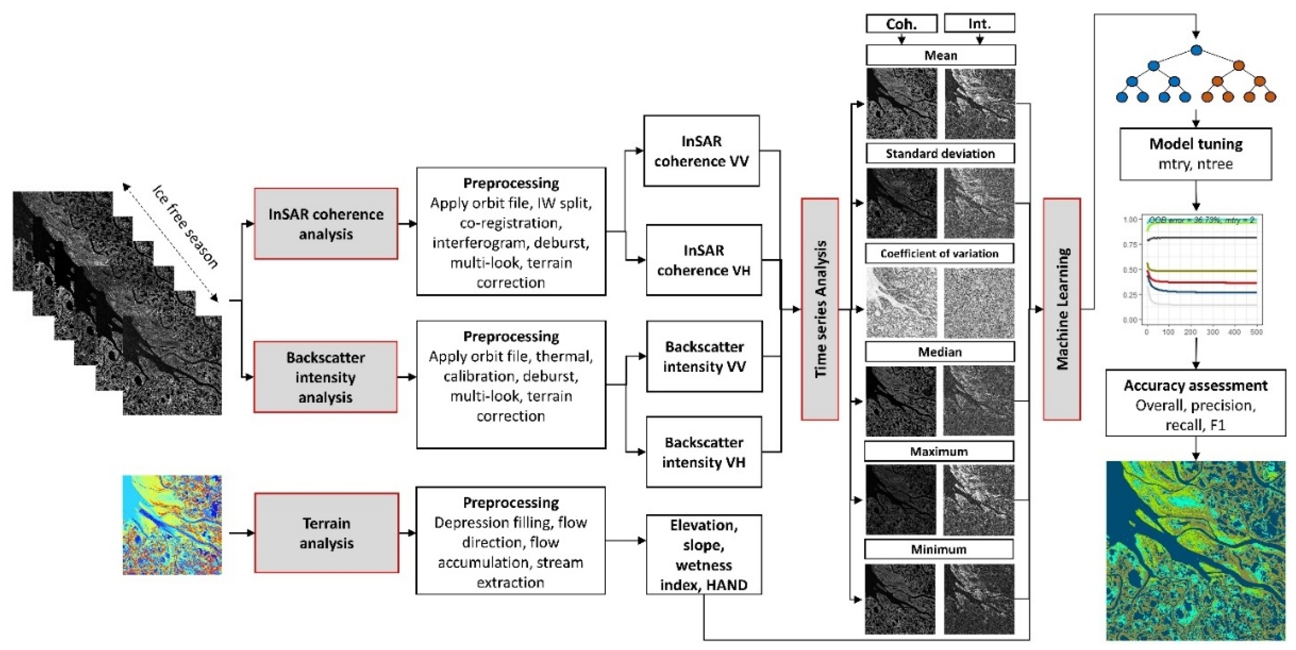
2.7. Sentinel-1 Image Processing

Backscatter intensity was first derived from each SAR scene using the Sentinel Application Platform (SNAP) toolbox [65]. Steps for deriving backscatter included thermal noise removal, radiometric calibration to sigma-nought (σ°), TOPSAR deburst, multi-looking, and geometric terrain correction. To obtain the backscattering coefficient (or normalized radar cross section) expressed in decibels, the following equation was used:
σ ° ( d B ) = 10 log 10 D N  
where DN is the Sentinel-1 scene pixels. Multi-looking was applied using a window of 4 × 1 in range and azimuth and terrain correction was completed using the ESA’s Copernicus GLO-30 DEM (1.0 arcseconds). Backscatter images were exported at 15 m spatial resolution.
Coherence was computed following [66]. Sub-swaths (i.e., IW1, IW2, and IW3) for each Sentinel-1 scene were processed separately, which was performed by splitting (i.e., selecting) the scenes using the S-1 TOPS Split operator in SNAP. Precise orbit information was then applied, followed by image pairs closest in acquisition date being co-registered; the earlier image was always designated as the ‘master’ image, and the later the ‘slave’. This produced five co-registered pairs, each with a temporal baseline of 12 days. Co-registration was completed based on satellite orbits along with information from the Copernicus GLO-30 DEM. The quality of the co-registration process was also increased by applying range and azimuth shift corrections using the Enhanced Spectral Diversity operator in SNAP. Interferogram processing for all co-registered pairs was completed using a coherence window of 10 × 3 pixels in the range and azimuth. The resulting coherence products had their burst seamlines corrected and then sub-swaths were merged with the S-1 TOPS Merge operator. Lastly, merged coherence products were multi-looked, terrain corrected, and exported at 15 m spatial resolution to match the intensity products (Figure 4).

2.8. Time-Series Statistical Descriptors

After preprocessing the Sentinel-1 images, we calculated several statistical metrics for each pixel in the time-series stack, for each polarization (VV and VH), and for both coherence and intensity. The statistical descriptors chosen largely followed earlier studies that performed similar analysis [30,31,67]. Multi-temporal, pixel-based statistical descriptors included mean, standard deviation, coefficient of variation, median, maximum, and minimum. These descriptors were derived using the raster package of R [68] and were used as machine learning model inputs.

2.9. Meteorological and Hydrometric Environmental Data

Historical environmental measurements were obtained across our study’s summer 2020 observational period. This included wind speed, precipitation, water level height, and discharge (Figure 5). All measurements were acquired from the Government of Canada’s Meteorological Service of Canada [69]. Hydrometric data (Figure 5a) were obtained from the Mackenzie River weather station and meteorological data (Figure 5b) from the Inuvik weather station. These environmental datasets aided in the interpretation of SAR intensity and coherence products and machine learning classification results.

2.10. Topographic Data

To aid in the classification of hydro-ecological conditions within our study area, a DEM was acquired. This was the Copernicus GLO-30 DEM [70], a Digital Surface Model (DSM) at 30 m resolution representing all features on the Earth’s surface. Several topographic metrics were derived from the DEM, as terrain morphology is a major influencer on water flow and pooling across landscapes. In addition to elevation, these metrics included slope, the wetness index [71], and Height Above Nearest Drainage (HAND [72]). All terrain metrics were processed using python scripting and with the WhiteboxTools geospatial data analysis platform [73]. Terrain metrics were resampled to 15 m and co-registered to the SAR imagery.

2.11. Random Forest Modelling

A machine learning approach was used to classify the combination of the SAR time-series data and terrain metrics. For this, we choose the Random Forest algorithm [74], which is very popular for remote sensing applications due to reported accuracies [75], ability to handle non-normally distributed datasets with high dimensionality and multi-collinearity [76], computational efficiency [77], and insensitivity to overfitting [78].
Random Forest is a robust, non-parametric ensemble learning algorithm that combines multiple decision trees models for problem solving using a bootstrap aggregating (i.e., bagging) method [79]. With bagging, each decision tree in the forest uses a random subset of samples from the dataset with replacement, resulting in each tree being unique. This training process uses two-thirds of the samples, while the remaining one-third is employed to independently cross-validate the model’s performance. This one-third of samples is referred to as out of bag (OOB). A final decision is then made by majority voting, whereby the membership class with the most prediction votes is selected. This leads to more accurate and stable classification results while mitigating overfitting [79]. The premise here is that a large ensemble of uncorrelated models will perform better than any single model.
To implement Random Forest, we set two key parameters—first was the number of randomly sampled variables used to split each node of a decision tree (mtry), and second is the number of generated decision trees (ntree). Rather than arbitrarily setting these parameters, we applied an algorithm-tuning process to find optimal values. A search function was used for mtry, whereby a minimum improvement in error (5%) was required for the search to continue until an optimal value was found, whereas ntree was assessed in incremental steps of 50 trees. Each parameter was assessed using OOB error. Random Forest tuning and classification were run using the randomForest and Caret packages in R [68].
A total of 11 Random Forest models were built in this study, each representing different optimally chosen model parameters (i.e., mtry and ntree) and different input data. These various models were then statistically examined, allowing for an understanding of the unique and combined contributions of SAR/InSAR and topographic data for hydro-ecological condition classification.

2.12. Accuracy Assessment

Random Forest model classifications were validated using the independent reference data polygons described in Section 2.3. Validation statistics included overall accuracy and per-class precision, recall, and F1 score. Statistical equations for these metrics are the following:
Overall   Accuracy = Number   of   Correctly   Classified   Samples Number   of   Total   Samples  
Precision = TP TP + FP  
Recall = TP TP + FN  
F 1   Score = 2 × Precision   ×   Recall Precision   +   Recall  
where TP are true positives (correct hit), FP false positives (false alarm), and FN false negatives (miss). F1 score is the harmonic mean (i.e., weighted average) of precision and recall.

3. Results and Discussion

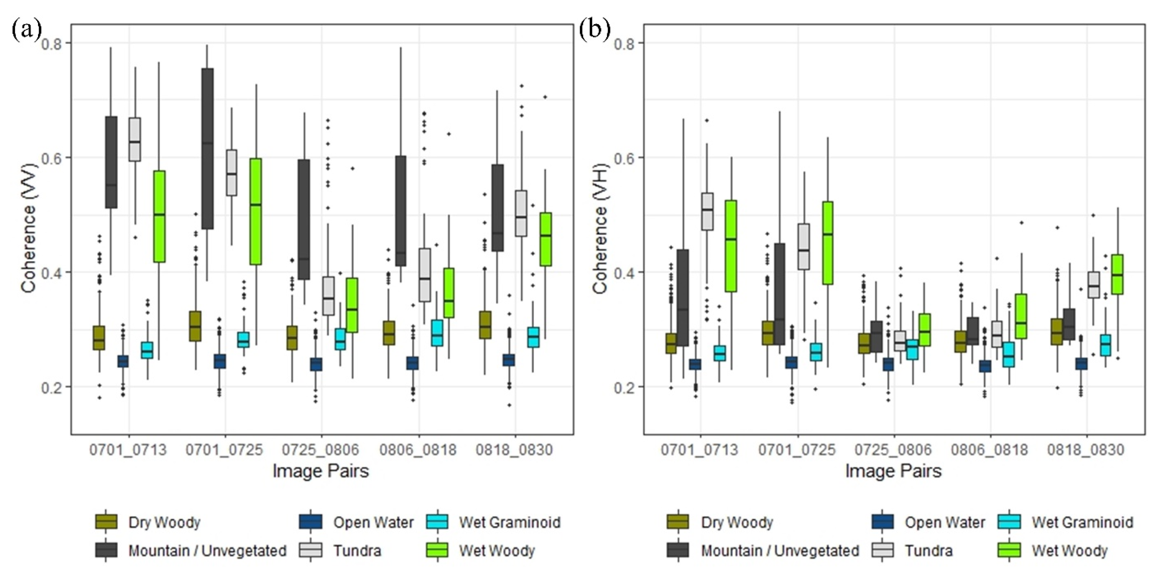
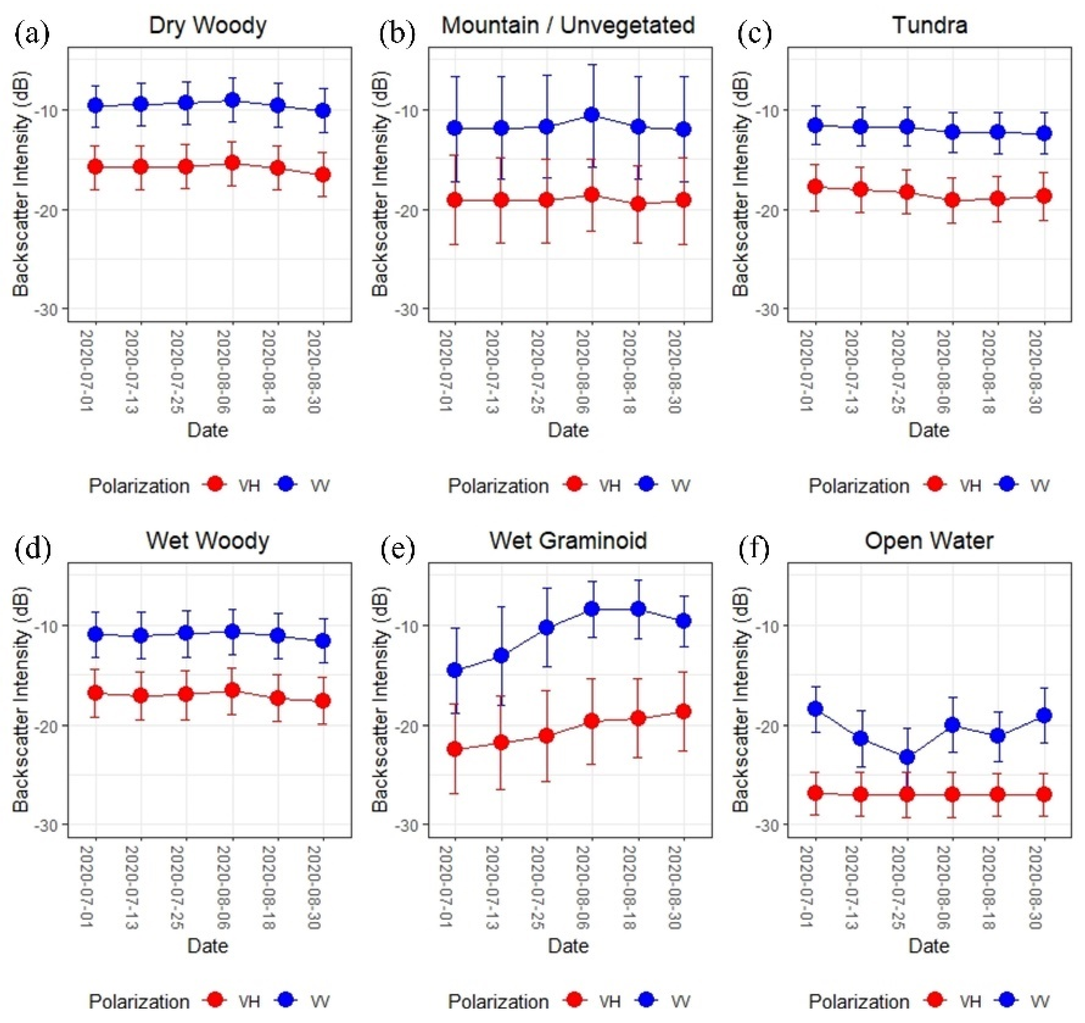
3.1. Temporal Observations of Coherence and Intensity

Prior to classification tests, the temporal evolution of SAR variables was observed. Figure 6 shows boxplots of time-series coherence for each class and image pair. For both VV and VH, coherence was found to be highest for most classes at the beginning of the ice-free season when discharge and water levels were greatest from runoff and increased precipitation (Figure 5). Coherence was then visibly lowest from 25 July to 6 August during the peak of the summer growing season. This suggests that flooded vegetation (e.g., wet woody areas) was maintaining a consistent double-bounce scattering during very wet periods [44,80,81], whereas vegetation phenological changes (i.e., green-up) and landscape drying result in decorrelation. Moreover, image pairs following this period (i.e., during August) showed a minor increasing trend in coherence during a period of relatively stable flow and water levels. For VV, the mountain/unvegetated class exhibited the highest coherence across the time series, followed by tundra and wet woody areas. Dry woody, wet graminoid, and open water areas all displayed rather low coherence in both VV and VH, around or below 0.3, and regardless of image pair. Open water in particular was very low with coherence values closer to 0.25 for both VV and VH. This is because smooth water bodies reflect the SAR signal away from the sensor, causing decorrelation. Nevertheless, these values of coherence were distinctly lower than other classes, producing a unique signal for this open water class. With VH, wet woody areas were the most coherent class, followed by tundra and mountain/unvegetated areas. Wet woody surface types were also far more coherent in VV then wet graminoid surface types. Other studies have noted a similar observation [29,31,82] in that flooded woody vegetation (e.g., in swamps or peatlands) produce greater return signal than herbaceous vegetation due to double-bounce scattering from trunks, branches, and stems. This allows for maintenance of coherence over longer temporal baselines.
Several studies have found the co-polarization channel (i.e., VV or HH) of a SAR to maintain better coherence than the cross-polarization channel (i.e., VH or HV), especially for hydrological applications such as inundation monitoring or wetland mapping [82,83,84] and regardless of wavelength (e.g., X-, C-, or L-band). This is because of the physics of Fresnel reflection from dielectric surfaces, which produces stronger backscatter in the HH channel than the VV [31]. This observation holds true in the case of this study, whereby all six hydro-ecological classes of interest maintained highest coherence in the co-polarization VV (Figure 6).
Figure 7 shows the time series of backscatter intensities (σ°) for each class of interest. The dry woody class had a relatively strong backscatter time series with VV (−9 dB) and VH (−16 dB) maximums on August 6 and lows on August 30, hence following the peak and conclusion of the growing season. Evidently, the backscatter is being influenced by the amount of leaves and branches (i.e., phenology) that cause volume scattering. Wet woody and mountain/unvegetated areas showed a similar trend with VV and VH backscatter intensity maximums on August 06. Tundra areas showed highest VV (−12 dB) and VH (−17 dB) backscatter intensities in early July, followed by a general and minor decline towards the end of August. Earlier onset of greenness for low shrub tundra landcovers has been observed in other remote sensing research [85]. Open water areas showed a pronounced difference in scattering with the lowest backscatter intensities of all classes in both SAR polarizations, although open water backscatter intensities were stable in the VH time series and highly variable from date to date in VV. Water bodies typically act as specular reflectors of SAR energy (i.e., forward scattering) due to their smooth surfaces [86]. However, wave development and fetch can disrupt the often flat/smooth target geometry of surface water, creating roughened surfaces leading to an increase in diffuse scattering. This was observed in the open water VV time series, in which the backscatter patterns were broadened, and intensities were highest on image acquisition dates corresponding with high wind speeds (Figure 5b). The wet graminoid class demonstrated the most signal variability, with a strong incline in intensity that reached a maximum VV backscatter of −8 dB on August 6 and VH backscatter of −18 dB on August 30. These distinct changes in the intensity time series are attributable to an increase in double-bounce scattering from tall, mature graminoids [87], which become more exposed as their phenology changes and water level heights decrease (Figure 8). Under such conditions, when the vegetation–water interface is pronounced creating a right angle, deflected backscatter from double-bounce (i.e., dihedral) scattering is high [88].

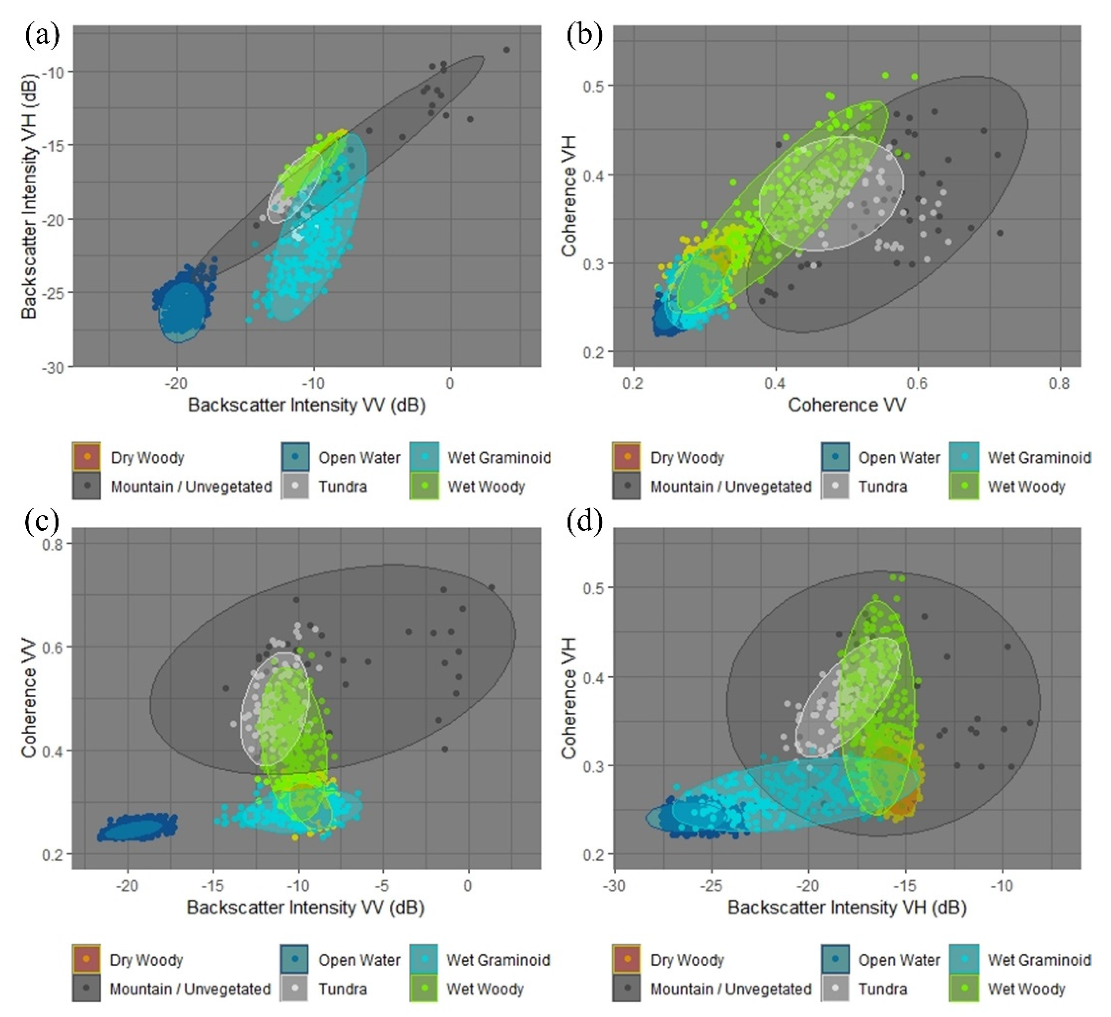
3.2. Feature Space Analysis

The feature space positions of each class were also visually observed, prior to classification, for SAR intensity and coherence variables. Figure 9 shows the feature space positions based on the mean value derived from the SAR time-series stacks. Open water showed a clear separability from all other classes when the VV intensity variable was plotted against other VH intensity and VV coherence (Figure 9a,c). Combining co- and cross-polarization VV and VH intensity separated the wet graminoid class well (Figure 9a). The wet woody class generally showed high overlap with several classes, both wet and dry, and in all feature space plots, although ellipse centers had less overlap when a combination of coherence and intensity variables were plotted (Figure 9c,d). The dry woody class feature cluster center was best separated using the cross-polarization VH coherence and VH intensity (Figure 9d). Mountain/unvegetated areas showed variable feature space positioning in all graphs, although were best separated using VV and VH coherence (Figure 9b). This aligns with the distinct and high coherence values seen in Figure 6. Tundra areas had relatively high overlap in all feature space plots, indicating the poorest separability. It is likely that a combination of topographic and SAR data, including both intensity and coherence in the co- and cross-polarization channels, is necessary for accurate classification and separability of these detailed hydro-ecological classes.

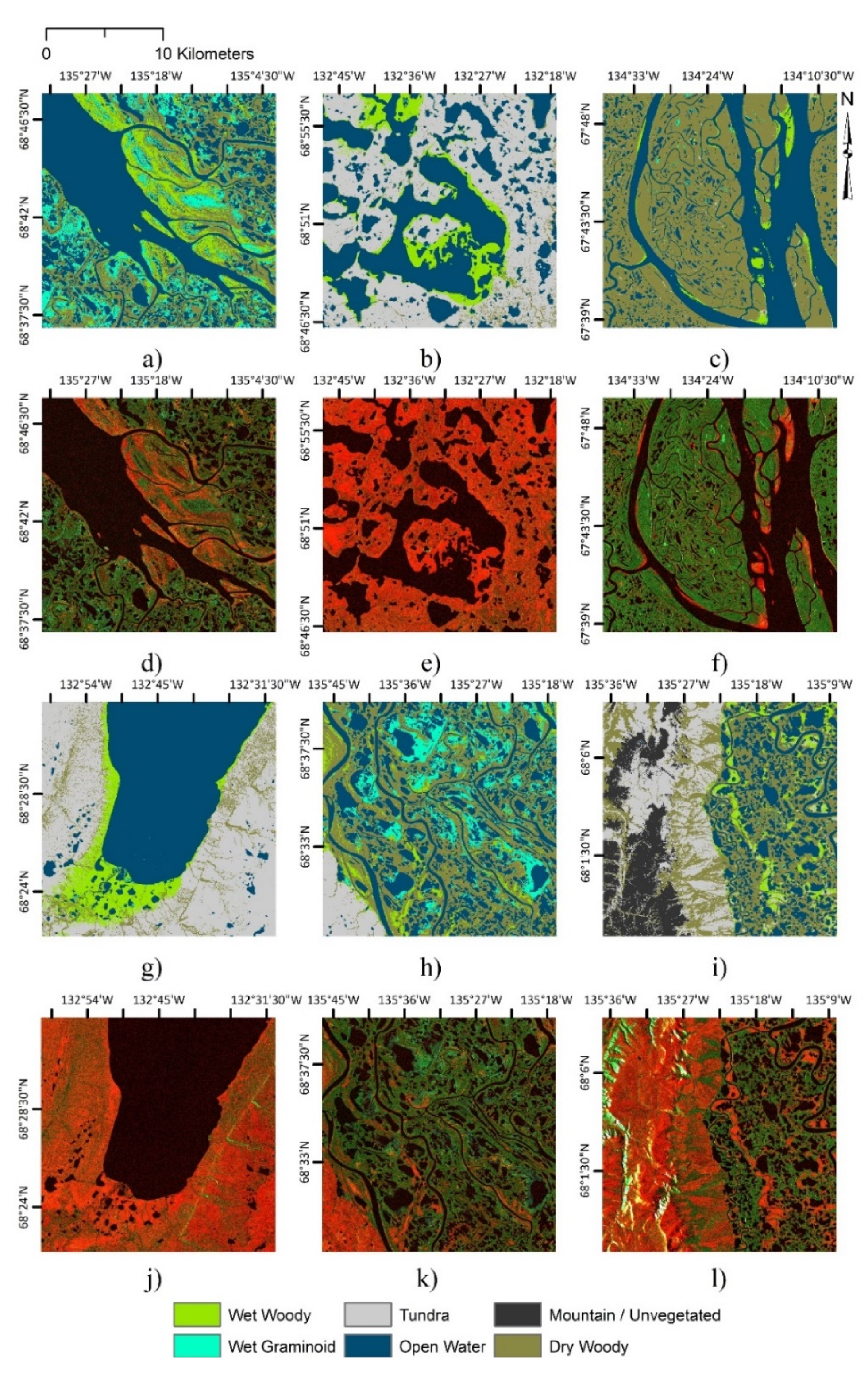
3.3. Classification Results

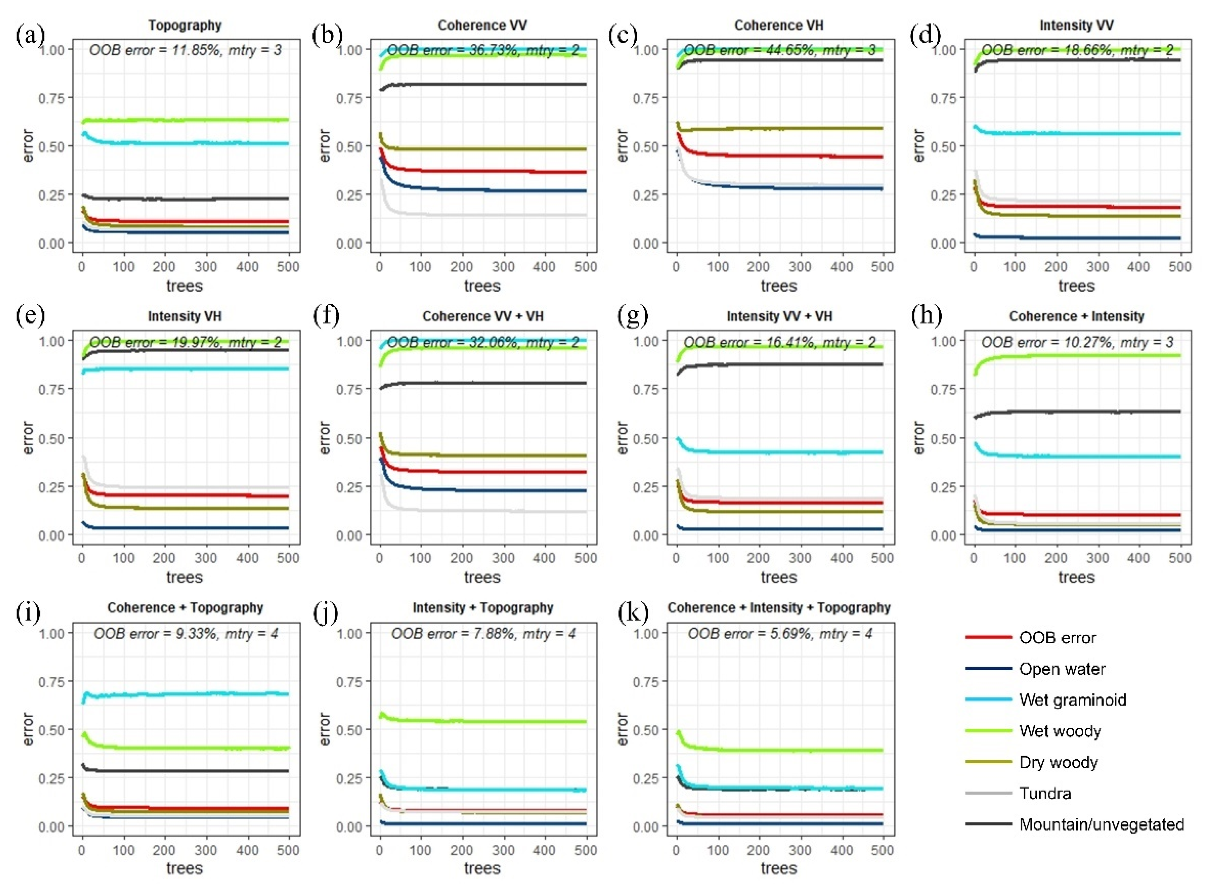
3.3.1. Effects of Model Hyperparameter Tuning

OOB data were used to obtain an internal and unbiased running estimate of classification error while incrementally adding trees to the forest [89]. This process allowed each Random Forest model to be fine-tuned based on the input variables. Figure 10a–k shows the results of the hyperparameter tuning process for all 11 Random Forest models. The graphs in Figure 10 show the average OOB model error rate curve along with per-class OOB error and the optimal mtry value. mtry values varied by model and ranged from 2 to 4. It is evident that an increase in model complexity (i.e., input variables) reduced overall model error. In general, VV and VH intensity (Figure 10d,e) produced lower OOB error rates than VV and VH coherence (Figure 10b,c). The synergistic use of coherence and intensity greatly decreased OOB error (Figure 10h), which aligns with the findings of previous studies that demonstrated InSAR and backscatter features to be complimentary for capturing hydrological patterns [30,44,61,90,91]. Inclusion of topographic data noticeably improved all Random Forest model performances, and even performed relatively well in isolation with an average OOB error rate of 11.85% (Figure 10a). This is because Arctic tundra biotic communities establish along environmental gradients, manifesting in clear areal patterns [92]. For low lying wet areas, topographic variations create plant zonation patterns in response to flooding frequency and duration, and soil moisture. The wettest areas of the Mackenzie Delta support shallow standing water, wetlands and lakes, whereas areas slightly elevated are subject to variable flooding or pulsing hydroperiods and the ensuing drainage processes, leading to the establishment of wet tolerant graminoids, shrubs, or trees, depending on elevation (i.e., wet graminoid or wet woody land covers [93]. The tussock-forming tundra areas are elevated higher outside the delta, with drier conditions that create their own micro-uplands that are distinct from wet areas. The Random Forest model using all intensity, coherence, and topographic variables produced a lowest OOB error of 5.69% (Figure 10k). In several Random Forest models, the wet woody class had the highest per-class OOB error, whereas open water was often the lowest.

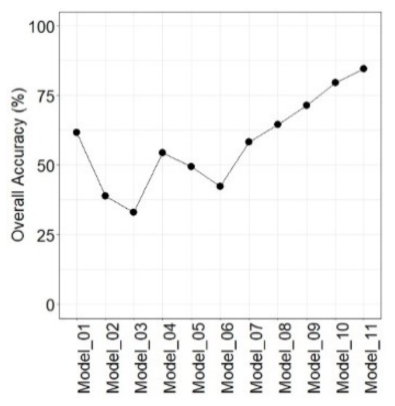
3.3.2. Classification Accuracy Assessments

Table 1 presents the independent per-class accuracy assessments for all 11 Random Forest model scenarios which varied based on input predictor variables. Overall, these independent assessments relate closely to the internal OOB model estimates presented in Figure 10. It is apparent from these statistical results that the combined use of intensity, coherence, and topography is required to accurately discriminate the complex hydro-ecological classes of the Mackenzie Delta and surrounding region. Each set of predictor variables offers differing characterization capabilities depending on their sensitivity to hydrological or ecological features.
For the wet classes (i.e., open water, wet graminoid, and wet woody), the co-polarization VV intensity (model 4) identified open water areas more accurately than coherence or topography with an F1 score of 0.860. In most cases, the open water class had the highest F1 score of the three wet classes, with model 11 achieving a highest F1 score of 0.955. This was followed by the wet graminoid class; wet graminoid areas were mostly incoherent (Figure 6) and thus VV or VH coherence could not identify them accurately. However, their intensity time series was considerably distinct (Figure 7), especially in VV where double-bounce scattering from flooded vegetation is more prevalent [94,95] depending on phenological stage. This was reflected in the VV intensity model (model 4) with an F1 score of 0.590. A highest F1 score of 0.921 was achieved with model 11 for the wet graminoid class. Overall, wet woody surface types were the most difficult class to classify. This is despite the relatively high coherence from this class (Figure 6). It was only once topographic data were combined with intensity or coherence data (models 9 and 10) that this class could be classified accurately. Model 11 achieved a highest F1 score of 0.682 for the wet woody class.
Most coherence or intensity only SAR scenarios (models 2 to 7) had difficulty classifying dry land cover types (i.e., dry woody, tundra, and mountain/unvegetated). The dry upland classes contained various combinations of short statured (i.e., height) shrubs, trees, or herbaceous vegetation, often producing minor differences in scattering mechanisms and absent of a strong and separable double-bounce signal more commonly associated with flooded states. Ullmann et al. [19] also noted the difficulty in using the VV/VH dual-polarization mode associated with Sentinel-1 for mapping of Tuktoyaktuk’s Arctic tundra landcover types; this earlier study suggested that a multi-frequency, multi-polarization, or multi-sensor approach is necessary for such applications. Nonetheless, the combination of both VV and VH coherence and intensity inputs (model 8) did result in relatively adequate F1 scores for the dry upland classes, ranging from 0.402 to 0.747. A multi-source approach with the inclusion of topographic information significantly reduced upland classification confusion, with model 11 resulting in F1 scores of 0.815–0.826 for these landcover types.
Figure 11 presents the overall accuracy statistics for all 11 Random Forest models. SAR intensity models (models 4 and 5) produced higher overall accuracies than SAR coherence models (models 2 and 3). In both cases, combined dual-polarimetric information (i.e., VV and VH; models 6 and 7) from intensity or coherence performed better than use of only one SAR channel (i.e., VV or VH; models 2 to 5). Several previous studies examining InSAR coherence for hydrological applications have included only the co-polarization channel of a SAR (i.e., VV or HH) with the assumption that this channel is more sensitive to surface water and flooded conditions [29,30,31]. While this is true in many instances, our study highlights the collective contributions of co- and cross-polarization SAR data for hydro-ecological characterization. This aspect of our study is important and can be attributed to the sensitivity of VH to vegetation canopy structures and volume scattering [95,96]. Merging intensity and coherence data (model 8) produced a relatively high overall accuracy of 64%. This SAR-only result is encouraging when considering the complexity of hydro-ecological landcover classes identified, the spatial extent of the Sentinel-1A scene, and that high-latitude regions are often cloudy with low-light conditions which limits the use of optical sensors. Mapping of Arctic tundra ecosystems therefore demands the use of SAR methods, which allow for better sampling due to cloud independence [97], although inclusion of topographic data significantly improved classification results, with model 11 achieving the highest overall accuracy of 84%.

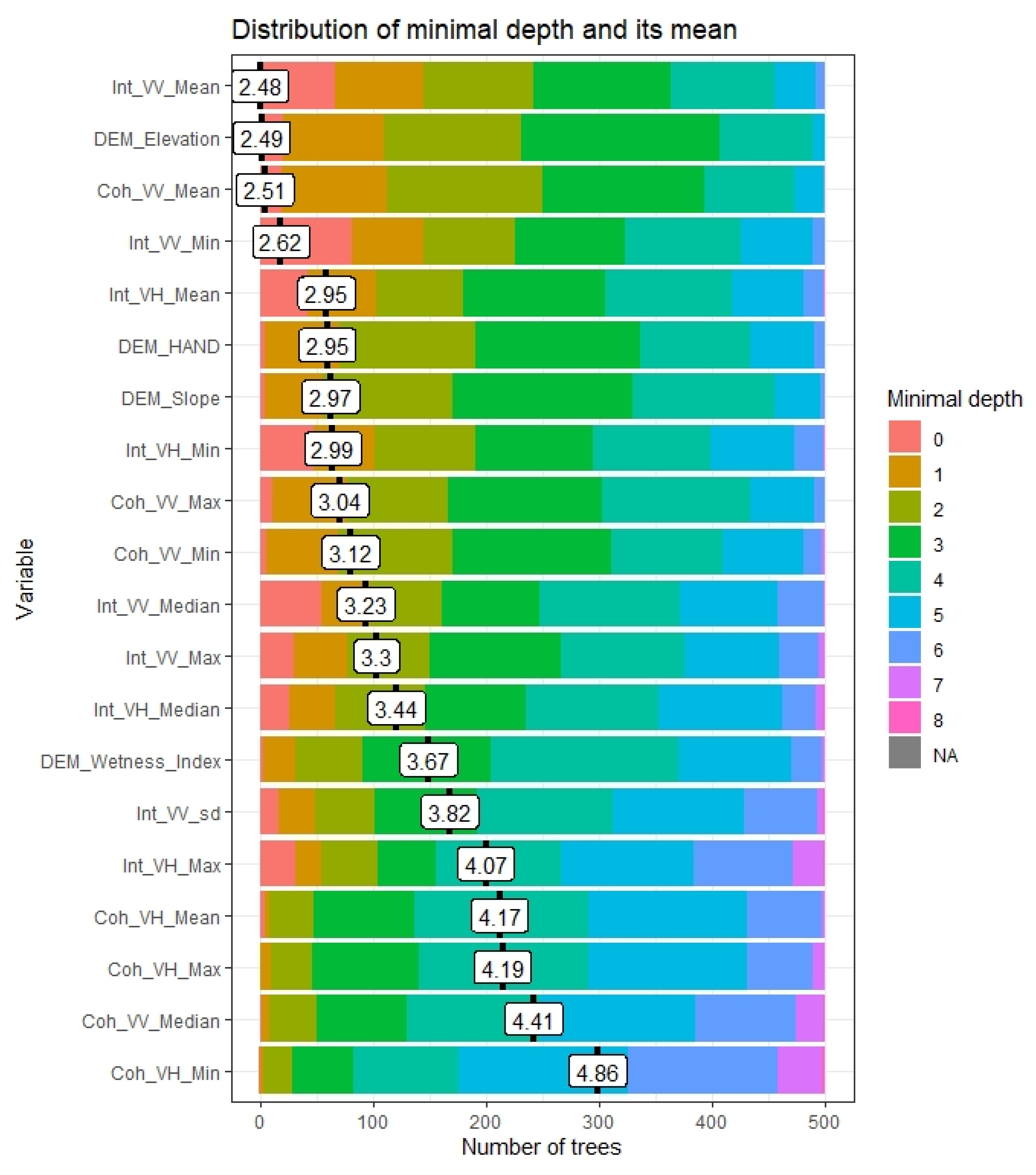
3.3.3. Variable Importance

A significant by-product of Random Forest calculations are measures of feature importance [79]. This algorithm characteristic is important for understanding parameter predictive power. Model 11 (Figure 12), which used all topographic and SAR time-series predictor variables, was selected for variable importance analysis since it resulted in the most significant overall accuracy (84%). For this study, we analyzed predictor power based on the distribution of the average minimal depth for each input variable [98]. The concept of minimal depth provides a measure of the distance of a variable to the root of the tree, thus allowing for an understanding of a variable’s role in the model structure and prediction. This is because at each node in the model, a random subset of predictor variables is used to make a split in the data; the most strongly associated variable is the one used to make the split. This indicates that variables closer to the root have stronger predictor power, are more important, and are most strongly associated with the dependent variables (i.e., output classes).
Figure 13 displays the top 20 variables from model 11 calculated using top trees. The smaller the mean minimal depth, the more important the predictor variable is. All four topographic variables, including elevation, HAND, slope, and the wetness index appeared as top 20 variables, further demonstrating the role topography plays in this Artic tundra landscape [92]. The most important predictor variable was the mean VV intensity, which is understandable due to VV’s sensitivity to hydrological conditions including moisture, flooding, and the accompanying double-bounce scattering mechanism. The mean VV coherence was also ranked very high at number three, furthering this understanding. Thus, the temporal signatures (i.e., those that are stable, and those that are dynamic) of VV coherence (e.g., Figure 6) and VV intensity (Figure 7) were captured well within the time-series statistical descriptors, resulting in strong classification predictive power. Nine of the top 20 variables were SAR intensity variables, indicating that SAR intensity provides greater predictor power in this landscape than SAR coherence.

3.3.4. Limitations and Future Analysis

Supervised data classification using machine learning algorithms such as Random Forest is a convenient and accurate means to land cover determination and delineation. However, there are various limitations that must be considered such as the potential of overfitting, difficulty in transferability from one site to another, run-time performance, and the requirements of time-consuming and sometimes costly training and testing data preparation [79], whether that be by in situ field methods, which are considered “gold standard”, or photointerpretation. The former is incredibly challenging in remote Arctic tundra environments, and the latter can be prone to human error and noise, even for an experienced image analyst. Regardless, quality training data of sufficient size (i.e., number of samples) is a requirement for machine learning algorithms such as Random Forests [99,100]. Without such a dataset, acceptable classification accuracies are difficult to achieve, giving rise to the problematic computational threat of “garbage-in-and-garbage-out” [101]. Our study presents a workflow that identifies the hydro-ecological state of Arctic tundra landcovers with both quantitatively and qualitatively (i.e., through visual inspection) acceptable results; however, it is recommended that future research assesses unsupervised clustering algorithms. Sometimes labelled sample data are not available, and thus unsupervised learning may present an alternative approach to thematic map generation. For example, in a recent study, Minotti et al. [102] used a Self-Organizing Map (SOM) neural network to cluster InSAR data from Sentinel-1 for wetland hydroperiod pattern.
Our mapping approach was also applied using pixel-based image analysis (PBIA) which, when applied to heterogeneous areas such as coastal deltas or Arctic tundra terrain, has limitations. For example, the heterogeneity in spatially near pixels, the occurrence of mixed pixels, and the effects of hydrological and ecological differences within a single class that may result in speckled noise [103]. Thus, it is suggested that this classification approach applies object-based image analysis (OBIA) in future work to address the heterogeneity of this dynamic landscape, as OBIA has shown to increase classification accuracies in many previous studies [75,104].
The availability of SAR satellites with open data policies and short revisit times, such as Sentinel-1A/1B, has made InSAR analysis more realizable for the geospatial community. This has resulted in many recent studies demonstrating the efficacy of time-series InSAR products over a variety of environments. Despite these promising results, readily available coherence products are still limited. For example, the popular cloud-computing platform Google Earth Engine contains only Ground Range Detected (GRD) Sentinel-1 data, meaning the phase information necessary for coherence is not available [105]. As remote sensing analysis moves farther away from local desktop processing, widespread adoption of both SAR intensity and coherence may be challenging, despite demonstrated applications. Moreover, the learning curve for InSAR processing may be steep for users more accustomed to conventional intensity products. Fortunately, there are some recent options designed to address the underutilization of InSAR products—one of which is the European Space Agency’s Geohazards Thematic Exploitation Platform (GEP), an R&D activity designed for large scale Earth observation data processing. Millard et al. [67] used this platform for Sentinel-1 InSAR processing and peatland mapping, although they noted that processing options were limited in comparison to a dedicated InSAR processing software (e.g., SNAP). Piter et al. [106] discuss other cloud-based platforms including CODE-DE and the Alaska Satellite Facility’s OpenSARLab and present their advantages and limitations. Improving the adoption of coherence measurements depends on the remote sensing community embracing InSAR cloud computing techniques, and thus future analysis should assess these resources accordingly. Such efforts would relieve SAR/InSAR users of big data downloads and processing time.
Lastly, while Sentinel-1 offers arguably the most consistent and reliable open-source time-series SAR data, its dual-polarimetric channels (i.e., VV and VH) and C-band wavelength are somewhat limiting characteristics. Of the co-polarized SAR channels, HH is favored because of its sensitivity to surface water and flooded conditions [95,107]. As a result, the HH polarization has shown to produce higher coherence than VV over wet environments such as coastal deltas [83]. The medium wavelength microwaves of Sentinel-1 (i.e., C-band) are also more sensitive to surface features which can mask significant coherence information [29]. In contrast, longer-wavelength L-band SAR data, being less sensitive to surface roughness due to canopy penetration capabilities, has proven fruitful for hydrological applications [44]. Future research should emphasize a combined multi-frequency SAR approach for hydro-ecological Arctic tundra mapping. Upcoming L-band SAR missions such as ALOS-4 and NASA-ISRO (NiSAR) offer promising opportunities for this [108].

4. Conclusions

In this study, we presented a machine learning workflow and preceding analysis using SAR/InSAR time-series products derived from Sentinel-1A for high-latitude hydro-ecological landcover characterization over one growing season. To our knowledge, very little previous research has been dedicated to this over Arctic tundra environments. Moreover, while knowledge of temporal landscape wetness is important for hydrological analysis, this information lacks the additional vegetation detail necessary for accurate greenhouse gas emission modelling, such as carbon and methane. Our study established a methodology capable of deriving this critical hydro-ecological information, which, considering northern ecosystems and their sensitivity to current climate warming, will be important for updating over forthcoming years as permafrost thaw continues to alter Arctic tundra conditions.
Key findings from our study included the following:
  • Wet woody, tundra, and mountain/unvegetated landcovers maintained the highest coherence over this study’s observation period, whereas wet graminoid, dry woody and open water landcovers showed the lowest coherence.
  • Coherence was generally highest at the beginning of this study’s observation period, when water levels and discharge were high, whereas decorrelation occurred from phenological changes and landscape drying.
  • Open water and wet graminoid landcovers demonstrated the most variability in backscatter intensity.
  • SAR backscatter intensity was able to classify hydro-ecological classes more accurately than InSAR coherence.
  • When intensity and coherence were combined, overall classification accuracies and per-class F1 score values were improved, suggesting that these SAR/InSAR variables are complimentary.
  • Inclusion of topographic variables improved all machine learning model outcomes, a result of topography’s control on Arctic tundra biotic communities.
  • A combination of coherence, intensity, and topographic variables resulted in a highest overall classification accuracy of 84%.
  • The co-polarized VV channel demonstrated stronger predictor power than the cross-polarized VH.
The Arctic tundra plays a significant role in global climate regulation, thus making the mapping and monitoring of these sensitive environments and their structure and function a significant task that is crucial for human adaptation. Our findings will help advance knowledge around these sensitive ecosystems, providing a means for status and trends updates at a suitable spatial and temporal detail.

Author Contributions

Conceptualization, M.A.M., M.O., B.D. and A.B.; SAR/InSAR processing, M.A.M.; analysis, M.A.M.; writing and original manuscript preparation, M.A.M.; manuscript review and editing, M.A.M., M.O., B.B., B.D. and A.B.; funding acquisition, B.D. and A.B. All authors have read and agreed to the published version of the manuscript.

Funding

We acknowledge the support of the Natural Sciences and Engineering Research Council of Canada (NSERC), [funding reference numbers RGPIN-2020-05743 and STPGP-521584]. Additional funding was provided by the Global Water Futures (GWF) research program through Northern Water Futures (NWF), which is funded by the Canada First Research Excellence Program.

Institutional Review Board Statement

Not applicable.

Informed Consent Statement

Not applicable.

Data Availability Statement

The data presented in this study are available on request from the corresponding author.

Acknowledgments

We would like to thank the NSERC and the GWF, along with Ducks Unlimited Canada (DUC) for providing spatially referenced field photographs collected within the study area. Lastly, the guidance and support by Canadian Center for Mapping and Earth Observation (CCMEO) staff was invaluable.

Conflicts of Interest

The authors declare no conflict of interest.

References

  1. IPCC. Climate Change 2021: The Physical Science Basis. Contribution of Working Group I to the Sixth Assessment Report of the Intergovernmental Panel on Climate Change; Masson-Delmotte, V., Zhai, P., Pirani, A., Connors, S.L., Péan, C., Berger, S., Caud, N., Chen, Y., Goldfarb, L.M.I., et al., Eds.; Cambridge University Press: Cambridge, UK, 2021. [Google Scholar]
  2. Berteaux, D.; Gauthier, G.; Domine, F.; Ims, R.A.; Lamoureux, S.F.; Lévesque, E.; Yoccoz, N. Effects of changing permafrost and snow conditions on tundra wildlife: Critical places and times. Arct. Sci. 2017, 3, 65–90. [Google Scholar] [CrossRef] [Green Version]
  3. Ford, J.; Smit, B. A framework for assessing the vulnerability of communities in the Canadian Arctic to risks associated with climate change. Arctic 2004, 57, 389–400. [Google Scholar] [CrossRef]
  4. Serreze, M.C.; Barry, R.G. Processes and impacts of Arctic amplification: A research synthesis. Glob. Planet. Chang. 2011, 77, 85–96. [Google Scholar] [CrossRef]
  5. Vonk, J.E.; Tank, S.E.; Bowden, W.B.; Laurion, I.; Vincent, W.F.; Alekseychik, P.; Amyot, M.; Billet, M.F.; Canário, J.; Cory, R.M.; et al. Reviews and syntheses: Effects of permafrost thaw on Arctic aquatic ecosystems. Biogeosciences 2015, 12, 7129–7167. [Google Scholar] [CrossRef] [Green Version]
  6. Junk, W.J.; An, S.; Finlayson, C.M.; Gopal, B.; Květ, J.; Mitchell, S.A.; Mitsch, W.J.; Robarts, R.D. Current state of knowledge regarding the world’s wetlands and their future under global climate change: A synthesis. Aquat. Sci. 2013, 75, 151–167. [Google Scholar] [CrossRef] [Green Version]
  7. Loranty, M.M.; Goetz, S.J. Shrub expansion and climate feedbacks in Arctic tundra. Environ. Res. Lett. 2012, 7, 011005. [Google Scholar] [CrossRef] [Green Version]
  8. Walvoord, M.A.; Voss, C.I.; Wellman, T.P. Influence of permafrost distribution on groundwater flow in the context of climate-driven permafrost thaw: Example from Yukon Flats Basin, Alaska, United States. Water Resour. Res. 2012, 48, 1–17. [Google Scholar] [CrossRef]
  9. Bring, A.; Fedorova, I.; Dibike, Y.; Hinzman, L.; Mård, J.; Mernild, S.H.; Prowse, T.; Semenova, O.; Stuefer, S.L.; Woo, M.K. Arctic terrestrial hydrology: A synthesis of processes, regional effects, and research challenges. J. Geophys. Res. G Biogeosci. 2016, 121, 621–649. [Google Scholar] [CrossRef]
  10. Tarnocai, C.; Canadell, J.G.; Schuur, E.A.G.; Kuhry, P.; Mazhitova, G.; Zimov, S. Soil organic carbon pools in the northern circumpolar permafrost region. Global Biogeochem. Cycles 2009, 23, 1–11. [Google Scholar] [CrossRef]
  11. Schuur, E.; McGuire, A.; Schadel, C.; Grosse, G.; Harden, J.; Hayes, D.; Hugelius, G.; Koven, C.; Puhry, P.; Lawrence, D.; et al. Climate change and the permafrost carbon feedback. Nature 2015, 520, 171–179. [Google Scholar] [CrossRef]
  12. Watts, J.D.; Kimball, J.S.; Bartsch, A.; McDonald, K.C. Surface water inundation in the boreal-Arctic: Potential impacts on regional methane emissions. Environ. Res. Lett. 2014, 9, 075001. [Google Scholar] [CrossRef]
  13. Du, J.; Watts, J.D.; Jiang, L.; Lu, H.; Cheng, X.; Duguay, C.; Farina, M.; Qiu, Y.; Kim, Y.; Kimball, J.S.; et al. Remote sensing of environmental changes in cold regions: Methods, achievements and challenges. Remote Sens. 2019, 11, 1952. [Google Scholar] [CrossRef] [Green Version]
  14. Beamish, A.; Raynolds, M.K.; Epstein, H.; Frost, G.V.; Macander, M.J.; Bergstedt, H.; Bartsch, A.; Kruse, S.; Miles, V.; Tanis, C.M.; et al. Recent trends and remaining challenges for optical remote sensing of Arctic tundra vegetation: A review and outlook. Remote Sens. Environ. 2020, 246, 111872. [Google Scholar] [CrossRef]
  15. A’Campo, W.; Bartsch, A.; Roth, A.; Wendleder, A.; Martin, V.S.; Durstewitz, L.; Lodi, R.; Wagner, J.; Hugelius, G. Arctic tundra land cover classification on the beaufort coast using the kennaugh element framework on dual-polarimetric TerraSAR-X imagery. Remote Sens. 2021, 13, 4780. [Google Scholar] [CrossRef]
  16. Chang, Q.; Zwieback, S.; DeVries, B.; Berg, A. Application of L-band SAR for mapping tundra shrub biomass, leaf area index, and rainfall interception. Remote Sens. Environ. 2022, 268, 112747. [Google Scholar] [CrossRef]
  17. Duguay, Y.; Bernier, M.; Lévesque, E.; Domine, F. Land cover classification in subarctic regions using fully polarimetric RADARSAT-2 data. Remote Sens. 2016, 8, 697. [Google Scholar] [CrossRef] [Green Version]
  18. Karlson, M.; Gålfalk, M.; Crill, P.; Bousquet, P.; Saunois, M.; Bastviken, D. Delineating Northern Peatlands Using Sentinel-1 Time Series and Terrain Indices from Local and Regional Digital Elevation Models. Remote Sens. Environ. 2019, 231, 111252. [Google Scholar] [CrossRef]
  19. Ullmann, T.; Banks, S.N.; Schmitt, A.; Jagdhuber, T. Scattering characteristics of X-, C- and L-band polsar data examined for the tundra environment of the Tuktoyaktuk Peninsula, Canada. Appl. Sci. 2017, 7, 595. [Google Scholar] [CrossRef] [Green Version]
  20. Buchelt, S.; Skov, K.; Ullmann, T. Sentinel-1 time series for mapping snow cover and timing of snowmelt in Arctic periglacial environments: Case study from the Zackenberg Valley, Greenland. Cryosph. Discuss. 2021, 16, 625–646. [Google Scholar] [CrossRef]
  21. Wang, L.; Marzahn, P.; Bernier, M.; Ludwig, R. Mapping permafrost landscape features using object-based image classification of multi-temporal SAR images. ISPRS J. Photogramm. Remote Sens. 2018, 141, 10–29. [Google Scholar] [CrossRef]
  22. Zwieback, S.; Berg, A.A. Fine-Scale SAR Soil Moisture Estimation in the Subarctic Tundra. IEEE Trans. Geosci. Remote Sens. 2019, 57, 4898–4912. [Google Scholar] [CrossRef]
  23. Jawak, S.D.; Bidawe, T.G.; Luis, A.J. A Review on Applications of Imaging Synthetic Aperture Radar with a Special Focus on Cryospheric Studies. Adv. Remote Sens. 2015, 4, 163–175. [Google Scholar] [CrossRef] [Green Version]
  24. Malenovský, Z.; Rott, H.; Cihlar, J.; Schaepman, M.E.; García-Santos, G.; Fernandes, R.; Berger, M. Sentinels for science: Potential of Sentinel-1, -2, and -3 missions for scientific observations of ocean, cryosphere, and land. Remote Sens. Environ. 2012, 120, 91–101. [Google Scholar] [CrossRef]
  25. Osmanoğlu, B.; Sunar, F.; Wdowinski, S.; Cabral-Cano, E. Time series analysis of InSAR data: Methods and trends. ISPRS J. Photogramm. Remote Sens. 2016, 115, 90–102. [Google Scholar] [CrossRef]
  26. Semenzato, A.; Pappalardo, S.E.; Codato, D.; Trivelloni, U.; de Zorzi, S.; Ferrari, S.; de Marchi, M.; Massironi, M. Mapping and monitoring urban environment through sentinel-1 SAR data: A case study in the Veneto region (Italy). ISPRS Int. J. Geo-Inf. 2020, 9, 375. [Google Scholar] [CrossRef]
  27. Chini, M.; Pelich, R.; Pulvirenti, L.; Pierdicca, N.; Hostache, R.; Matgen, P. Sentinel-1 InSAR Coherence to Detect Floodwater in Urban Areas: Houston and Hurricane Harvey as A Test Case. Remote Sens. 2019, 11, 107. [Google Scholar] [CrossRef] [Green Version]
  28. Béjar-Pizarro, M.; Notti, D.; Mateos, R.M.; Ezquerro, P.; Centolanza, G.; Herrera, G.; Bru, G.; Sanabria, M.; Solari, L.; Duro, J.; et al. Mapping vulnerable urban areas affected by slow-moving landslides using Sentinel-1InSAR data. Remote Sens. 2017, 9, 876. [Google Scholar] [CrossRef] [Green Version]
  29. Amani, M.; Poncos, V.; Brisco, B.; Foroughnia, F.; Delancey, E.R.; Ranjbar, S. Insar coherence analysis for wetlands in alberta, canada using time-series sentinel-1 data. Remote Sens. 2021, 13, 3315. [Google Scholar] [CrossRef]
  30. Canisius, F.; Brisco, B.; Murnaghan, K.; Van Der Kooij, M.; Keizer, E. SAR backscatter and InSAR coherence for monitoring wetland extent, flood pulse and vegetation: A study of the Amazon lowland. Remote Sens. 2019, 11, 720. [Google Scholar] [CrossRef] [Green Version]
  31. Brisco, B.; Ahern, F.; Murnaghan, K.; White, L.; Canisus, F.; Lancaster, P. Seasonal change in wetland coherence as an aid to wetland monitoring. Remote Sens. 2017, 9, 158. [Google Scholar] [CrossRef] [Green Version]
  32. Kim, J.W.; Lu, Z.; Gutenberg, L.; Zhu, Z. Characterizing hydrologic changes of the Great Dismal Swamp using SAR/InSAR. Remote Sens. Environ. 2017, 198, 187–202. [Google Scholar] [CrossRef]
  33. Battaglia, M.J.; Banks, S.; Behnamian, A.; Bourgeau-Chavez, L.; Brisco, B.; Corcoran, J.; Chen, Z.; Huberty, B.; Klassen, J.; Knight, J.; et al. Multi-source eo for dynamic wetland mapping and monitoring in the great lakes basin. Remote Sens. 2021, 13, 599. [Google Scholar] [CrossRef]
  34. Wang, L.; Marzahn, P.; Bernier, M.; Ludwig, R. Sentinel-1 InSAR measurements of deformation over discontinuous permafrost terrain, Northern Quebec, Canada. Remote Sens. Environ. 2020, 248, 111965. [Google Scholar] [CrossRef]
  35. Strozzi, T.; Antonova, S.; Günther, F.; Mätzler, E.; Vieira, G.; Wegmüller, U.; Westermann, S.; Bartsch, A. Sentinel-1 SAR interferometry for surface deformation monitoring in low-land permafrost areas. Remote Sens. 2018, 10, 1360. [Google Scholar] [CrossRef] [Green Version]
  36. Rouyet, L.; Lauknes, T.R.; Christiansen, H.H.; Strand, S.M.; Larsen, Y. Seasonal dynamics of a permafrost landscape, Adventdalen, Svalbard, investigated by InSAR. Remote Sens. Environ. 2019, 231, 111236. [Google Scholar] [CrossRef]
  37. Frison, P.L.; Fruneau, B.; Kmiha, S.; Soudani, K.; Dufrêne, E.; Le Toan, T.; Koleck, T.; Villard, L.; Mougin, E.; Rudant, J.P. Potential of Sentinel-1 data for monitoring temperate mixed forest phenology. Remote Sens. 2018, 10, 2094. [Google Scholar] [CrossRef] [Green Version]
  38. Pulella, A.; Santos, R.A.; Sica, F.; Posovszky, P.; Rizzoli, P. Multi-temporal sentinel-1 backscatter and coherence for rainforest mapping. Remote Sens. 2020, 12, 847. [Google Scholar] [CrossRef] [Green Version]
  39. Sun, X.; Wang, B.; Xiang, M.; Zhou, L.; Jiang, S. Forest height estimation based on P-band pol-inSAR modeling and multi-baseline inversion. Remote Sens. 2020, 12, 1319. [Google Scholar] [CrossRef] [Green Version]
  40. Chen, Z.; Montpetit, B.; Banks, S.; White, L.; Behnamian, A.; Duffe, J.; Pasher, J. Insar monitoring of arctic landfast sea ice deformation using l-band alos-2, c-band radarsat-2 and sentinel-1. Remote Sens. 2021, 13, 4570. [Google Scholar] [CrossRef]
  41. Marbouti, M.; Praks, J.; Antropov, O.; Rinne, E.; Leppäranta, M. A study of landfast ice with Sentinel-1 repeat-pass interferometry over the Baltic Sea. Remote Sens. 2017, 9, 833. [Google Scholar] [CrossRef] [Green Version]
  42. Dierking, W.; Lang, O.; Busche, T. Sea ice local surface topography from single-pass satellite InSAR measurements: A feasibility study. Cryosphere 2017, 11, 1967–1985. [Google Scholar] [CrossRef] [Green Version]
  43. Zebker, H.; Villasenor, J. Decorrelation in interferometric radar echoes. IEEE Trans. Geosci. Remote Sens. 1992, 30, 950–959. [Google Scholar] [CrossRef] [Green Version]
  44. Mohammadimanesh, F.; Salehi, B.; Mahdianpari, M.; Brisco, B.; Motagh, M. Multi-temporal, multi-frequency, and multi-polarization coherence and SAR backscatter analysis of wetlands. ISPRS J. Photogramm. Remote Sens. 2018, 142, 78–93. [Google Scholar] [CrossRef]
  45. Pepe, A.; Calò, F. A review of interferometric synthetic aperture RADAR (InSAR) multi-track approaches for the retrieval of Earth’s Surface displacements. Appl. Sci. 2017, 7, 1264. [Google Scholar] [CrossRef] [Green Version]
  46. Bamler, R.; Hartl, P. Synthetic aperture radar interferometry. Inverse Probl. 1998, 88, R1–R54. [Google Scholar] [CrossRef]
  47. Marsh, P.; Pomeroy, J.W. Meltwater fluxes at an arctic forest-tundra site. Hydrol. Process. 1996, 10, 1383–1400. [Google Scholar] [CrossRef]
  48. Marsh, P.; Onclin, C.; Russell, M. A multi-year hydrological data set for two research basins in the Mackenzie Delta region, NW Canada. In Proceedings of the Northern Research Basins Water Balance, Victoria, BC, Canada, 15–19 March 2004; pp. 205–212. [Google Scholar]
  49. Shi, X.; Marsh, P.; Yang, D. Warming spring air temperatures, but delayed spring streamflow in an Arctic headwater basin. Environ. Res. Lett. 2015, 10, 064003. [Google Scholar] [CrossRef]
  50. Macdonald, R.; Wong, C.; Erickson, P. The distribution of nutrients in the southeastern Beaufort Sea: Implications for water circulation and primary production. J. Geophys. Res. Ocean. 1987, 92, 2939–2952. [Google Scholar] [CrossRef]
  51. Rood, S.B.; Kaluthota, S.; Philipsen, L.J.; Rood, N.J.; Zanewich, K.P. Increasing discharge from the Mackenzie River system to the Arctic Ocean. Hydrol. Process. 2017, 31, 150–160. [Google Scholar] [CrossRef]
  52. Burn, C. Mackenzie Delta: Canada’s principle arctic delta. In Landscapes and Landforms of Western Canada; Slaymaker, O., Ed.; Springer: Gewerbestrasse, Switzerland, 2016; pp. 321–334. [Google Scholar]
  53. Heginbottom, J. Canada-Permafrost; Plate 2.1 (MCR 4177); Walter de Gruyter: Berlin, Germany, 1995. [Google Scholar] [CrossRef]
  54. Macdonald, R.W.; Yu, Y. The Mackenzie Estuary of the Arctic ocean. Handb. Environ. Chem. 2006, 5, 91–120. [Google Scholar]
  55. Marsh, P.; Hey, M. The Flooding Hydrology of Mackenzie Delta Lakes near Inuvik. Arctic 1989, 42, 41–49. [Google Scholar] [CrossRef] [Green Version]
  56. Gill, D. The Point Bar Environment in the Mackenzie River Delta. Can. J. Earth Sci. 1972, 9, 1382–1393. [Google Scholar] [CrossRef]
  57. Pohl, S.; Davison, B.; Marsh, P.; Pietroniro, A. Modelling spatially distributed snowmelt and meltwater runoff in a small arctic catchment with a hydrology land-surface scheme (WATCLASS). Atmos. Ocean. 2005, 43, 193–211. [Google Scholar] [CrossRef]
  58. Rouse, J.W.; Hass, R.H.; Schell, J.A.; Deering, D.W. Monitoring vegetation systems in the great plains with ERTS. Third Earth Resour. Technol. Satell. Symp. 1973, 1, 309–317. [Google Scholar]
  59. Muhuri, A.; Manickam, S.; Bhattacharya, A. Snehmani snow cover mapping using polarization fraction variation with temporal RADARSAT-2 C-band full-polarimetric SAR data over the Indian Himalayas. IEEE J. Sel. Top. Appl. Earth Obs. Remote Sens. 2018, 11, 2192–2209. [Google Scholar] [CrossRef]
  60. Park, S.E. Variations of microwave scattering properties by seasonal freeze/thaw transition in the permafrost active layer observed by ALOS PALSAR polarimetric data. Remote Sens. 2015, 7, 17135–17148. [Google Scholar] [CrossRef] [Green Version]
  61. Adeli, S.; Salehi, B.; Mahdianpari, M.; Quackenbush, L.J.; Brisco, B.; Tamiminia, H.; Shaw, S. Wetland monitoring using SAR Data: A meta-analysis and comprehensive review. Remote Sens. 2020, 12, 2190. [Google Scholar] [CrossRef]
  62. Liu, F.; Jiao, L.; Hou, B.; Yang, S. POL-SAR Image Classification Based on Wishart DBN and Local Spatial Information. IEEE Trans. Geosci. Remote Sens. 2016, 54, 3292–3308. [Google Scholar] [CrossRef]
  63. Touzi, R.; Lopes, A.; Bruniquel, J.; Vachon, P.W. Coherence estimation for SAR imagery. IEEE Trans. Geosci. Remote Sens. 1999, 37, 135–149. [Google Scholar] [CrossRef] [Green Version]
  64. Seymour, M.S.; Cumming, I.G. Maximum likelihood estimation for SAR interferometry. In Proceedings of the International Geoscience and Remote Sensing Symposium (IGARSS), Pasadena, CA, USA, 8–12 August 1994; Volume 4, pp. 2272–2274. [Google Scholar]
  65. European Space Agency. Science Tool Exploitation Platform—Sentinel Application Platform (STEP-SNAP). Available online: http://step.esa.int/main/toolboxes/snap/ (accessed on 1 June 2021).
  66. Braun, A.; Veci, L. TOPS Interferometry Tutorial; ESA: Paris, France, 2021. [Google Scholar]
  67. Millard, K.; Kirby, P.; Nandlall, S.; Behnamian, A.; Banks, S.; Pacini, F. Using growing-season time series coherence for improved peatland mapping: Comparing the contributions of Sentinel-1 and RADARSAT-2 coherence in full and partial time series. Remote Sens. 2020, 12, 2465. [Google Scholar] [CrossRef]
  68. R Core Team. R: A Language and Environment for Statistical Computing; R Foundation for Statistical Computing: Vienna, Austria, 2017. [Google Scholar]
  69. Meteorological Service of Canada. Historical Climate Data. Available online: https://climate.weather.gc.ca/ (accessed on 1 June 2021).
  70. European Space Agency. Copernicus DEM-Global and European Digital Elevation Model (COP-DEM). Available online: https://spacedata.copernicus.eu/web/cscda/dataset-details?articleId=394198 (accessed on 1 June 2021).
  71. Beven, K.J.; Kirkby, M.J. A physically based, variable contributing area model of basin hydrology. Hydrol. Sci. Bull. 1979, 24, 43–69. [Google Scholar] [CrossRef] [Green Version]
  72. Nobre, A.D.; Cuartas, L.A.; Hodnett, M.; Rennó, C.D.; Rodrigues, G.; Silveira, A.; Waterloo, M.; Saleska, S. Height Above the Nearest Drainage-A hydrologically relevant new terrain model. J. Hydrol. 2011, 404, 13–29. [Google Scholar] [CrossRef] [Green Version]
  73. Lindsay, J. Whitebox GAT: A case study in geomorphometric analysis. Comput. Geosci. 2016, 95, 75–84. [Google Scholar] [CrossRef]
  74. Breiman, L. Random Forests. Mach. Learn. 2001, 45, 5–32. [Google Scholar] [CrossRef] [Green Version]
  75. Merchant, M.; Warren, R.; Edwards, R.; Kenyon, J. An Object-Based Assessment of Multi-Wavelength SAR, Optical Imagery and Topographical Datasets for Operational Wetland Mapping in Boreal Yukon, Canada. Can. J. Remote Sens. 2019, 45, 308–332. [Google Scholar] [CrossRef]
  76. Kloiber, S.M.; Macleod, R.D.; Smith, A.J.; Knight, J.F.; Huberty, B.J. A Semi-Automated, Multi-Source Data Fusion Update of a Wetland Inventory for East-Central Minnesota, USA. Wetlands 2015, 35, 335–348. [Google Scholar] [CrossRef]
  77. Miao, X.; Heaton, J.S.; Zheng, S.; Charlet, D.A.; Liu, H. Applying tree-based ensemble algorithms to the classification of ecological zones using multi-temporal multi-source remote-sensing data. Int. J. Remote Sens. 2012, 33, 1823–1849. [Google Scholar] [CrossRef]
  78. Guan, H.; Li, J.; Chapman, M.; Deng, F.; Ji, Z.; Yang, X. Integration of orthoimagery and lidar data for object-based urban thematic mapping using random forests. Int. J. Remote Sens. 2013, 34, 5166–5186. [Google Scholar] [CrossRef]
  79. Belgiu, M.; Dragut, L. Random Forest in Remote Sensing: A Review of Applications and Future Directions. ISPRS J. Photogramm. Remote Sens. 2016, 114, 24–31. [Google Scholar] [CrossRef]
  80. Alsdorf, D.E.; Smith, L.C.; Melack, J.M. Amazon floodplain water level changes measured with interferometric SIR-C radar. IEEE Trans. Geosci. Remote Sens. 2001, 39, 423–431. [Google Scholar] [CrossRef]
  81. Liao, H.; Wdowinski, S.; Li, S. Regional-scale hydrological monitoring of wetlands with Sentinel-1 InSAR observations: Case study of the South Florida Everglades. Remote Sens. Environ. 2020, 251, 112051. [Google Scholar] [CrossRef]
  82. Kim, S.W.; Wdowinski, S.; Amelung, F.; Dixon, T.H.; Won, J.S. Interferometric coherence analysis of the everglades Wetlands, South Florida. IEEE Trans. Geosci. Remote Sens. 2013, 51, 5210–5224. [Google Scholar] [CrossRef]
  83. Hong, S.H.; Wdowinski, S. Evaluation of the quad-polarimetric Radarsat-2 observations for the wetland InSAR application. Can. J. Remote Sens. 2012, 37, 484–492. [Google Scholar] [CrossRef] [Green Version]
  84. Kim, J.W.; Lu, Z.; Lee, H.; Shum, C.K.; Swarzenski, C.M.; Doyle, T.W.; Baek, S.H. Integrated analysis of PALSAR/Radarsat-1 InSAR and ENVISAT altimeter data for mapping of absolute water level changes in Louisiana wetlands. Remote Sens. Environ. 2009, 113, 2356–2365. [Google Scholar] [CrossRef]
  85. Stow, D.A.; Hope, A.; McGuire, D.; Verbyla, D.; Gamon, J.; Huemmrich, F.; Houston, S.; Racine, C.; Sturm, M.; Tape, K.; et al. Remote sensing of vegetation and land-cover change in Arctic Tundra Ecosystems. Remote Sens. Environ. 2004, 89, 281–308. [Google Scholar] [CrossRef] [Green Version]
  86. Dabboor, M.; Brisco, B. Wetland Monitoring and Mapping Using Synthetic Aperture Radar. In Wetlands Management-Assessing Risk and Sustainable Solutions; IntechOpen: Berlin, Germany, 2018. [Google Scholar]
  87. Chen, Y.; Qiao, S.; Zhang, G.; Xu, Y.J.; Chen, L.; Wu, L. Investigating the potential use of Sentinel-1 data for monitoring wetland water level changes in China’s Momoge National Nature Reserve. PeerJ 2020, 8, e8616. [Google Scholar] [CrossRef]
  88. White, L.; Brisco, B.; Dabboor, M.; Schmitt, A.; Pratt, A. A collection of SAR methodologies for monitoring wetlands. Remote Sens. 2015, 7, 7615–7645. [Google Scholar] [CrossRef] [Green Version]
  89. Cutler, D.R.; Edwards, T.C.; Beard, K.H.; Cutler, A.; Hess, K.T.; Gibson, J.; Lawler, J.J. Random forests for classification in ecology. Ecology 2007, 88, 2783–2792. [Google Scholar] [CrossRef]
  90. Zhang, M.; Li, Z.; Tian, B.; Zhou, J.; Tang, P. The backscattering characteristics of wetland vegetation and water-level changes detection using multi-mode SAR: A case study. Int. J. Appl. Earth Obs. Geoinf. 2016, 45, 1–13. [Google Scholar] [CrossRef]
  91. Zhang, X.; Chan, N.W.; Pan, B.; Ge, X.; Yang, H. Mapping flood by the object-based method using backscattering coefficient and interference coherence of Sentinel-1 time series. Sci. Total Environ. 2021, 794, 148388. [Google Scholar] [CrossRef]
  92. Walker, D.A. Hierarchical subdivision of Artic tundra based on vegetation response to climate, parent material and topography. Glob. Chang. Biol. 2000, 6, 19–34. [Google Scholar] [CrossRef] [PubMed] [Green Version]
  93. Young, F. Geological and geographical guide to the Mackenzie Delta area. In Proceedings of the CSPG International Conference Facts and Principles of World Oil Occurrence, Calgary, AB, Canada, 26–28 June 1978; pp. 110–121. [Google Scholar]
  94. Tsyganskaya, V.; Martinis, S.; Marzahn, P. Detection of Temporary Flooded Vegetation Using Sentinel-1 Time Series Data. Remote Sens. 2018, 10, 1286. [Google Scholar] [CrossRef] [Green Version]
  95. Tsyganskaya, V.; Martinis, S.; Marzahn, P.; Ludwig, R.; Tsyganskaya, V.; Martinis, S.; Marzahn, P.; Ludwig, R. SAR-based detection of flooded vegetation–A review of characteristics and approaches. Int. J. Remote Sens. 2018, 39, 2255–2293. [Google Scholar] [CrossRef]
  96. Freeman, A.; Durden, S. A Three-Component Scattering Model for Polarimetric SAR Data. IEEE Trans. Geosci. Remote Sens. 1998, 36, 963–973. [Google Scholar] [CrossRef] [Green Version]
  97. Bartsch, A.; Höfler, A.; Kroisleitner, C.; Trofaier, A. Land cover mapping in northern high latitude permafrost regions with satellite data: Achievements and remaining challenges. Remote Sens. 2016, 8, 979. [Google Scholar] [CrossRef] [Green Version]
  98. Paluszynska, A.; Biecek, P.; Jiang, Y. Random Forest Explainer: Explaining and Visualizing Random Forests in Terms of Variable Importance. R Package Version 0.9 2017. Available online: https://github.com/ModelOriented/randomForestExplainer (accessed on 1 December 2021).
  99. Millard, K.; Richardson, M. On the importance of training data sample selection in random forest image classification: A case study in peatland ecosystem mapping. Remote Sens. 2015, 7, 8489–8515. [Google Scholar] [CrossRef] [Green Version]
  100. Gislason, P.O.; Benediktsson, J.A.; Sveinsson, J.R. Random forests for land cover classification. Pattern Recognit. Lett. 2006, 27, 294–300. [Google Scholar] [CrossRef]
  101. Thapa, A.; Bradford, L.; Strickert, G.; Yu, X.; Johnston, A.; Watson-Daniels, K. “Garbage in, garbage out” Does not hold true for indigenous community flood extent modeling in the prairie pothole region. Water 2019, 11, 2486. [Google Scholar] [CrossRef] [Green Version]
  102. Minotti, P.G.; Rajngewerc, M.; Alí Santoro, V.; Grimson, R. Evaluation of SAR C-band interferometric coherence time-series for coastal wetland hydropattern mapping. J. S. Am. Earth Sci. 2021, 106, 102976. [Google Scholar] [CrossRef]
  103. Dronova, I. Object-Based Image Analysis in Wetland Research: A Review. Remote Sens. 2015, 7, 6380–6413. [Google Scholar] [CrossRef] [Green Version]
  104. Fu, B.; Wang, Y.; Campbell, A.; Li, Y.; Zhang, B.; Yin, S.; Xing, Z.; Jin, X. Comparison of Object-Based and Pixel-Based Random Forest Algorithm for Wetland Vegetation Mapping Using High Spatial Resolution GF-1 and SAR Data. Ecol. Indic. 2017, 73, 105–117. [Google Scholar] [CrossRef]
  105. Tamiminia, H.; Salehi, B.; Mahdianpari, M.; Quackenbush, L.; Adeli, S.; Brisco, B. Google Earth Engine for geo-big data applications: A meta-analysis and systematic review. ISPRS J. Photogramm. Remote Sens. 2020, 164, 152–170. [Google Scholar] [CrossRef]
  106. Piter, A.; Vassileva, M.; Haghshenas Haghighi, M.; Motagh, M. Exploring cloud-based platforms for rapid insar time series analysis. Int. Arch. Photogramm. Remote Sens. Spat. Inf. Sci. 2021, 43, 171–176. [Google Scholar] [CrossRef]
  107. Mahdavi, S.; Salehi, B.; Granger, J.; Amani, M.; Brisco, B.; Huang, W. Remote sensing for wetland classification: A comprehensive review. GISci. Remote Sens. 2018, 55, 623–658. [Google Scholar] [CrossRef]
  108. Liao, T.H.; Simard, M.; Denbina, M.; Lamb, M.P. Monitoring water level change and seasonal vegetation change in the coastal wetlands of louisiana using L-band time-series. Remote Sens. 2020, 12, 2351. [Google Scholar] [CrossRef]
Figure 1. Study area map, located in the Northwest Territories, Canada. The study area in red represents the Sentinel-1A image stack footprint. The extent of the Mackenzie Delta is displayed for reference. TVRS = Trail Valley Creek Research Station.
Remotesensing 14 01123 g001
Figure 2. Field photos of landcover classes. (ac) Open water, (df) wet graminoid, (gi) wet woody, (jl) dry woody, (mo) mountain/unvegetated, and (pr) tundra. Photos were provided by Ducks Unlimited Canada (DUC).
Remotesensing 14 01123 g002
Figure 3. Reference data derived from high-resolution satellite imagery used for model training and testing. (a) WorldView-2 scene, (b) NDVI layer derived from WorldView-2 scene, (c) reference polygons derived from WorldView-2 scene, (d) WorldView-3 scene, (e) NDVI layer derived from WorldView-3 scene, (f) reference polygons derived from WorldView-3 scene, (gh) zoomed-in examples of reference data, and (i) spectral signatures of landcover classes derived from the WorldView imagery.
Remotesensing 14 01123 g003
Figure 4. Flowchart for deriving hydro-ecological classes using Sentinel-1 and GLO-30 DEM data, time-series analysis, and machine learning.
Remotesensing 14 01123 g004
Figure 5. Environmental conditions in relation to Sentinel-1 SAR acquisition dates. (a) Hydrometric data, and (b) meteorological data.
Remotesensing 14 01123 g005
Figure 6. Time-series evolution of coherence for all land cover classes across the 2020 growing season. Image pairs are labelled as monthday_monthday. (a) VV coherence, and (b) VH coherence.
Remotesensing 14 01123 g006
Figure 7. Time-series evolution of VV and VH SAR backscatter intensity. (ac) dry classes, and (df) wet classes.
Remotesensing 14 01123 g007
Figure 8. WorldView-3 false color example of wet graminoid areas highlighted in yellow. These emergent dominated areas are associated with shallow wetlands and lakes, where water levels are very dynamic.
Remotesensing 14 01123 g008
Figure 9. Feature space scatterplots for SAR intensity and coherence variables. Plots were created using the mean time-series descriptor. Ellipses represent the 95% confidence-level regions. (a) VH and VV intensity, (b) VH and VV coherence, (c) VV intensity and VV coherence, and (d) VH intensity and VH coherence.
Remotesensing 14 01123 g009
Figure 10. Internal classification error rates for each Random Forest model based on hyperparameter fine tuning. Model inputs are labelled above each graph. The red line is the average out-of-bag (OOB) model error. The optimal model mtry value is also labelled along with average model error rates.
Remotesensing 14 01123 g010
Figure 11. Overall accuracy values for each Random Forest model scenario (see Table 1 for model inputs). Overall accuracy was assessed using independent testing data.
Remotesensing 14 01123 g011
Figure 12. 84% overall accuracy. (df) and (jl) are RGB composites of R = mean intensity, G = standard deviation intensity, and B = mean coherence. (ac) and (gi) are the corresponding classified data.
Remotesensing 14 01123 g012
Figure 13. The distribution of the minimal depth among trees of the forest for the top 20 predictor variables from model 11. Minimal depth is represented by distinct colors. The mean minimal depth is depicted by the black vertical line and the value is labelled. The X axis ranges from 0 to the maximum number of trees in which any predictor variable was used for splitting.
Remotesensing 14 01123 g013
Table 1. Summarized per-class accuracy assessment statistics, displayed as a heatmap. OW = open water; WG = wet graminoid; WW = wet woody; DW = dry woody; TU = tundra; MU = mountain/unvegetated; DEM = digital elevation model; C = coherence; I = intensity.
ModelInputsStatisticOWWGWWDWTUMU
1DEMPrecision0.6250.9520.5870.4290.7250.993
Recall0.9260.3720.0840.8770.8750.461
F1 score0.7460.0840.1480.5770.7930.630
2CVVPrecision0.4410.0000.0560.3180.3760.811
Recall0.7520.0000.0020.5040.8550.128
F1 score0.5560.0000.0040.3900.5220.222
3CVHPrecision0.3660.0000.6250.2650.3290.880
Recall0.7530.0000.0100.3990.6850.044
F1 score0.4920.0000.0190.3190.4450.083
4IVVPrecision0.7620.9540.0000.4080.4430.929
Recall0.9880.4270.0000.8770.8040.026
F1 score0.8600.5900.0000.5570.5710.050
5IVHPrecision0.6420.7510.0000.4420.3980.735
Recall0.9830.1410.0000.8800.7830.025
F1 score0.7760.2370.0000.5880.5270.048
6CVV, CVHPrecision0.4850.0000.0880.3560.4000.899
Recall0.8170.0000.0030.5920.8860.142
F1 score0.6090.0000.0060.4450.5520.246
7IVV, IVHPrecision0.7540.9110.1670.4630.4570.940
Recall0.9880.5790.0040.8980.8130.079
F1 score0.8560.7080.0080.6110.5850.145
8CVV, CVH, IVV, IVHPrecision0.7970.9320.1530.6080.4570.962
Recall0.9930.5710.0090.9680.9440.254
F1 score0.8840.7080.0170.7470.6160.402
9CVV, CVH, DEMPrecision0.6120.9730.9080.6140.7310.991
Recall0.9560.3120.5290.9380.9300.534
F1 score0.7460.4720.6680.7420.8180.694
10IVV, IVH, DEMPrecision0.9140.9900.8660.5700.7490.993
Recall0.9930.8310.3210.9340.9060.725
F1 score0.9520.9030.4680.7080.8200.838
11CVV, CVH, IVV, IVH, DEMPrecision0.9190.9930.9190.7000.7370.993
Recall0.9940.8590.5420.9750.9390.706
F1 score0.9550.9210.6820.8150.8260.826
Publisher’s Note: MDPI stays neutral with regard to jurisdictional claims in published maps and institutional affiliations.

