
Modifications for the Differential Evolution Algorithm


Department of Informatics and Telecommunications, University of Ioannina, 47150 Kostaki Artas, Greece
*
Author to whom correspondence should be addressed.
Symmetry 2022, 14(3), 447; https://doi.org/10.3390/sym14030447
Submission received: 27 January 2022
/
Revised: 11 February 2022
/
Accepted: 19 February 2022
/
Published: 23 February 2022
(This article belongs to the Special Issue Emerging Applications of Machine Learning in Smart Systems Symmetry)
Abstract
:Differential Evolution (DE) is a method of optimization used in symmetrical optimization problems and also in problems that are not even continuous, and are noisy and change over time. DE optimizes a problem with a population of candidate solutions and creates new candidate solutions per generation in combination with existing rules according to discriminatory rules. The present work proposes two variations for this method. The first significantly improves the termination of the method by proposing an asymptotic termination rule, which is based on the differentiation of the average of the function values in the population of DE. The second modification proposes a new scheme for a critical parameter of the method, which improves the method’s ability to better explore the search space of the objective function. The proposed variations have been tested on a number of problems from the current literature, and from the experimental results, it appears that the proposed modifications render the method quite robust and faster even in large-scale problems.
1. Introduction
The location of the global minimum of a continuous and differentiable function is formulated as:
where the set S is defined as:
In the recent literature, there are a plethora of real-world problems that can be formulated as global optimization problems, such as problems from physics [1,2,3,4], chemistry [5,6,7], economics [8,9], etc. Furthermore, global optimization methods are used in many symmetry problems [10,11,12,13,14].There are a variety of proposed methods to handle the global minimum problem, such as Adaptive Random Search [15], Competitive Evolution [16], Controlled Random Search [17], Simulated Annealing [18,19,20], Genetic Algorithms [21,22], Bee optimization [23,24], Ant Colony Optimization [25], Particle Swarm Optimization [26], Differential Evolution [27], etc. Recently, many works have appeared that take advantage of the GPU processing units to implement parallel global optimization methods [28,29,30]. This work introduces two major modifications for the Differential Evolution (DE) method that aim to speed up the algorithm and reduce the total number of function evaluations required by the method. The DE method initially creates a population of candidate solutions and, through a series of iterations, creates new solutions by combining the previous ones. The method does not require any prior knowledge of the derivative and is, therefore, quite fast with low memory requirements. Moreover, the method has been used in various symmetry problems from the relevant literature, such as community detection [31], structure prediction of materials [32], motor fault diagnosis [33], automatic clustering techniques [34], etc.
After a literature review, it was found that differential evolution is used in several areas and many modifications of the original algorithm have been introduced in the recent literature. More specifically, in the research of Zongjun et al. [35], genetic and differential calculus algorithms were used to optimize the parameters of two models aimed at estimating evapotranspiration in three regions, and it was found that the performance of evolution algorithms was better than the genetic algorithm. Other research focused on a case study of a cellular neural network aimed at generating fractional classes of neurons. The best solutions from differential calculus and accelerated particle swarm optimization (APSO) are presented concretely in the work of Tlelo-Cuautle et al. [36]. Another article [37] proposes a regeneration framework based on space search adaptation (ARSA), which can be integrated into different variants of different evolutions to address the problems of early convergence and population stability faced by differential calculus. Another interesting variation of the method is the Bernstain Search Differential Evolution Algorithm [38] for optimizing numerical functions.
The differential evolution method was also applied to energy science. Specifically, the article of Liang et al. [39] evaluates the parameters of solar photovoltaic models through a self-adjusting differential evolution. Similarly, in the study of Peng et al. [40], differential evolution is used for the prediction of electricity prices. Furthermore, differential evolution was also incorporated in a neural architecture search [41]. The DE method has been applied with success to neural network training [42,43,44], to the Traveling Salesman Problem [45,46], training of RBF neural networks [47,48,49], and optimization of the Lennard Jones potential [50,51]. The DE method has also been successfully combined with other techniques for machine learning applications, such as classification [52,53], feature selection [54,55], deep learning [56,57], etc.
The rest of this article is organized as follows: In Section 2, the base DE algorithm, as well as the proposed modifications, are presented. In Section 3, the test functions used in the experiments are presented along with the experimental results. Finally, in Section 4, some conclusions are presented.
2. Modifications
This section starts with a detailed description of the DE method and continues with the modifications suggested in this article. The first modification is a new stopping rule, which measures the difference of the mean of the function values between the iterations of the algorithm. The second modification suggests a new scheme for a critical parameter of the DE algorithm called Differential Weight.
2.1. The Base Algorithm
The DE algorithm has been studied by various researchers in the recent literature, such as the Compact Differential Evolution [58], a self adaptive DE [59] where the critical parameters of the method are adapted from previous generations, a fuzzy adaptive DE method [60] where fuzzy login is employed to adapt the parameters of the method, parallel Differential Evolution [61] with a self adaptation mechanism for the critical parameters of the DE method, etc. A survey of the recent advances in differential evolutions can be found in the work of Das et al. [62]. The base DE algorithm has the steps described in Algorithm 1.
| Algorithm 1: DE algorithm. |
|
2.2. The New Termination Rule
Typically, the DE method is terminated when a predefined number of iterations is reached. This can be extremely inefficient in some problems and, in others, it can lead to premature termination, i.e., termination before the total minimum is found. In the work of Ali et al. [63], a different termination rule is proposed i.e., terminate when:
where is the function value of the worst agent in the population, is the function value of the best agent, and is a small positive number.
In the proposed termination rule, the average function value of the population is calculated in each iteration. If this value does not change significantly for a repetitive number of iterations, then it is very likely that the method may not discover a new global minimum and should therefore be terminated. Hence, in every generation t, we measure the quantity:
and the termination rule is defined as: terminate if for a predefined number of M generations.
2.3. The New Differential Weight
The differential weight initially proposed in the DE algorithm was a static value, which means that some tuning is required in order to discover the global minimum in every optimization function. Ali et al. [63] proposed an adaptation mechanism for this parameter in that the algorithm should search in larger spaces in the the first generations, and become more focused in later generations. The mechanism proposed is expressed as:
The current work proposes a stochastic mechanism similar to the crossover operation of the Genetic algorithms. The proposed scheme is expressed as:
where is a random number. The proposed scheme, as with the randomness introduced by the method DE will be able to better explore the search space of the objective function and find with greater accuracy and speed the global minimum. In addition, this scheme has been used successfully in Genetic Algorithms.
3. Experiments
In order to determine the effectiveness of the proposed modifications, a series of experiments were performed on known functions from the relevant literature [64,65]. The choice of these functions was made as they are widely used in the literature by many researchers [66,67,68,69], they have quite a complex structure, and in many cases, they have a large number of dimensions that make them ideal for studying and testing.
The experiments were divided into two major categories. In the first category, all the schemes for the Differential Weight were tested using the termination rule of Equation (2), and in the second category, the same schemes were tested using the proposed termination criterion. Furthermore, after every successful termination, the local optimization method BFGS [70] was applied in order to get even closer to the global minimum.
3.1. Test Functions
The descriptions of the test functions used in the experiments are as follows:
- Bf1 (Bohachevsky 1) function defined as:with . The value of global minimum is 0.0.
- Bf2 (Bohachevsky 2) function defined as:with . The value of the global minimum is 0.0.
- Branin function. The function is defined by with . The value of global minimum is 0.397887.with . The value of global minimum is −0.352386.
- CM function. The Cosine Mixture function is given by the equation:where . For our experiments we used .
- Camel function. The function is given by:
- Easom function. The function is given by the equation:with
- Exponential function, defined as:The global minimum is located at with value . In our experiments we used this function with .
- Goldstein and Price functionThe function is given by the equation:with . The global minimum is located at with value 3.0.
- Griewank2 function. The function is given by:The global minimum is located at the with value 0.
- Gkls function. , is a function with w local minima, described in [71] with and n a positive integer between 2 and 100. The value of the global minimum is −1 and in our experiments we have used and .
- Hansen function. , .
- Hartman 3 function. The function is given by:with and and
- Hartman 6 function.with and and
- Potential function. The molecular conformation corresponding to the global minimum of the energy of N atoms interacting via the Lennard-Jones potential [72] is used as a test case here. The function to be minimized is given by:In the current experiments three different cases were studied:
- Rastrigin function. The function is given by:The global minimum is located at with value −2.0.
- Rosenbrock function.This function is given by:The global minimum is located at the with . In our experiments we used this function with .
- Shekel 7 function.
- Shekel 5 function.
- Shekel 10 function.
- Sinusoidal function. The function is given by:The global minimum is located at with . In our experiments we used and and the corresponding functions are denoted by the labels SINU4, SINU8, SINU16 and SINU32, respectively.
- Test2N function. This function is given by the equation:The function has in the specified range and in our experiments we used . The corresponding values of global minimum is −156.664663 for , −195.830829 for , −234.996994 for and −274.163160 for .
- Test30N function. This function is given by:with , with local minima in the searc space. For our experiments we used .
3.2. Experimental Results
The experiments were performed 30 times with different seeds for the random generator each time for every test function and the avarage function was measured and reported. The code was implemented in ANSI C++ and the random generator used was the function drand48() of the C programming languages. The execution environment was an Intel Xeon E5-2630 multi-core machine. The parameters used in the experiments are shown in Table 1. The experiments where the stopping rule of Equation (2) was used are outlined in Table 2, and the experiments with the proposed stopping rule are listed in Table 3. The numbers in the cells represent average function calls. The fraction in parentheses stands for the fraction of runs where the global optimum was found. If this number is missing then the global minimum was discovered in every independent run (100% success). The column STATIC represents the static value for the differential weight , the column ALI stands for the mechanism given in the Equation (4), and lastly, the column PROPOSED stands for the proposed scheme given in Equation (5).
From the experiments, we observe that the two proposed variations drastically reduce the required number of function calls. Moreover, the proposed changes did not seem to affect the average performance of the method, as it remained high in all cases. The effect of the proposed scheme for the differential weight is presented graphically in Figure 1, where we plot the average function calls for the functions ROSENBROCK4, ROSENBROCK8, and ROSENBROCK16 using the three schemes of differential weights. Furthermore, in the plot of Figure 2, the average calls for the same functions are shown with both the proposed scheme for the differential weights and the proposed termination rule. It is evident that the combination of both modifications reduced, even more, the average number of function calls required to locate the global minimum of the test functions. To show the effectiveness of the modifications, Figure 3 presents the total time for 30 executions on an I7 computer with LINUX DEBIAN and 16 GB of memory. The comparison was made between the initial method with the ALI termination criterion, the proposed termination criterion (first modification), and the proposed termination criterion together with the proposed weight scheme. The proposed modifications significantly reduced the number of calls and also the required execution time. To compare the proposed scheme for the differential weight with the other two methods, the Wilcoxon signed-rank test was used. The results obtained with this statistical test are shown in Figure 4.
4. Conclusions
In this text, two main additions to the DE method are presented. In the first, an asymptotic termination rule was introduced and used successfully, even in multidimensional problems. This rule is based on the observation that from one point onwards the average of the functional values of the agents does not change. This means that either the algorithm has already found the global minimum or its further continuation will have no meaning.
In the second case, a stochastic scheme was used to produce the differential weight. This scheme helped the algorithm to better explore the search space of the objective function without the need for more calls to the objective function.
The proposed modifications significantly speed up the original method in terms of function calls, in most cases. Each of the proposed modifications can be used separately or together in the DE method. If used together, there is a large reduction in the number of required function calls that reach up to 80% without problems, and in the reliability of the method and its ability to successfully find the total minimum.
The DE method can also be used in cases of optimization problems with constraints as long as there is a change in the original problem so that the constraints are included in the function with the usage for example Langrage multipliers.
Author Contributions
V.C., I.G.T., A.T. and E.K. conceived of the idea and methodology and supervised the technical part regarding the software for the estimation of the global minimum of multidimensional symmetric and asymmetric functional problems. V.C. and I.G.T. conducted the experiments, employing several different functions, and provided the comparative experiments. A.T. performed the statistical analysis. V.C. and all other authors prepared the manuscript. V.C., E.K. and I.G.T. organized the research team and A.T. supervised the project. All authors have read and agreed to the published version of the manuscript.
Funding
We acknowledge support of this work from the project “Immersive Virtual, Augmented and Mixed Reality Center of Epirus” (MIS 5047221) which is implemented under the Action “Reinforcement of the Research and Innovation Infrastructure”, funded by the Operational Programme “Competitiveness, Entrepreneurship and Innovation” (NSRF 2014-2020) and co-financed by Greece and the European Union (European Regional Development Fund).
Institutional Review Board Statement
Not applicable.
Informed Consent Statement
Not applicable.
Data Availability Statement
Not applicable.
Acknowledgments
The experiments of this research work were performed at the high performance computing system established at the Knowledge and Intelligent Computing Laboratory, Department of Informatics and Telecommunications, University of Ioannina, acquired with the project “Educational Laboratory equipment of TEI of Epirus” with MIS 5007094 funded by the Operational Programme “Epirus” 2014–2020, by ERDF and national finds.
Conflicts of Interest
All authors declare that they have no has no conflict of interest.
References
- Kudyshev, Z.A.; Kildishev, A.V.; Boltasseva, V.M.S.A. Machine learning–assisted global optimization of photonic devices. Nanophotonics 2021, 10, 371–383. [Google Scholar] [CrossRef]
- Ding, X.L.; Li, Z.Y.; Meng, J.H.; Zhao, Y.X.; Sheng, G.H. Density-functional global optimization of (LA2O3)n Clusters. J. Chem. Phys. 2012, 137, 214311. [Google Scholar] [CrossRef] [PubMed]
- Morita, S.; Naoki, N. Global optimization of tensor renormalization group using the corner transfer matrix. Phys. Rev. B 2021, 103, 045131. [Google Scholar] [CrossRef]
- Heiles, S.; Johnston, R.L. Global optimization of clusters using electronic structure methods. Int. J. Quantum Chem. 2013, 113, 2091–2109. [Google Scholar] [CrossRef]
- Yang, Y.; Pan, T.; Zhang, J. Global Optimization of Norris Derivative Filtering with Application for Near-Infrared Analysis of Serum Urea Nitrogen. Am. J. Anal. Chem. 2019, 10, 143–152. [Google Scholar] [CrossRef] [Green Version]
- Grebner, C.; Becker, J.; Weber, D.; Engels, B. Tabu search based global optimization algorithms for problems in computational Chemistry. J. Cheminf. 2012, 4, 10. [Google Scholar] [CrossRef]
- Dittner, M.; Müller, J.; Aktulga, H.M.; Hartke, B.J. Efficient global optimization of reactive force-field parameters. Comput. Chem. 2015, 36, 1550–1561. [Google Scholar] [CrossRef]
- Zhao, W.; Wang, L.; Zhang, Z. Supply-Demand-Based Optimization: A Novel Economics-Inspired Algorithm for Global Optimization. IEEE Access 2019, 7, 73182–73206. [Google Scholar] [CrossRef]
- Mishra, S.K. Global Optimization of Some Difficult Benchmark Functions by Host-Parasite Co-Evolutionary Algorithm. Econ. Bull. 2013, 33, 1–18. [Google Scholar]
- Freisleben, B.; Merz, P. A genetic local search algorithm for solving symmetric and asymmetric traveling salesman problems. In Proceedings of the IEEE International Conference on Evolutionary Computation, Nagoya, Japan, 20–22 May 1996; pp. 616–621. [Google Scholar]
- Grbić, R.; Nyarko, E.K.; Scitovski, R. A modification of the DIRECT method for Lipschitz global optimization for a symmetric function. J. Glob. Optim. 2013, 57, 1193–1212. [Google Scholar] [CrossRef]
- Scitovski, R. A new global optimization method for a symmetric Lipschitz continuous function and the application to searching for a globally optimal partition of a one-dimensional set. J. Glob. Optim. 2017, 68, 713–727. [Google Scholar] [CrossRef]
- Kim, Y. An unconstrained global optimization framework for real symmetric eigenvalue problems. Appl. Num. Math. 2019, 144, 253–275. [Google Scholar] [CrossRef]
- Osaba, E.; Yang, X.S.; Diaz, F.; Lopez-Garcia, P.; Carballedo, R. An improved discrete bat algorithm for symmetric and asymmetric Traveling Salesman Problems. Eng. Appl. Artif. Intell. 2016, 49, 59–71. [Google Scholar] [CrossRef]
- Bremermann, H.A. A method for unconstrained global optimization. Math. Biosci. 1970, 9, 1–15. [Google Scholar] [CrossRef]
- Jarvis, R.A. Adaptive global search by the process of competitive evolution. IEEE Trans. Syst. Man Cybergen. 1975, 75, 297–311. [Google Scholar] [CrossRef]
- Price, W.L. Global Optimization by Controlled Random Search. Comput. J. 1977, 20, 367–370. [Google Scholar] [CrossRef] [Green Version]
- Kirkpatrick, S.; Gelatt, C.D.; Vecchi, M.P. Optimization by simulated annealing. Science 1983, 220, 671–680. [Google Scholar] [CrossRef]
- Van Laarhoven, P.J.M.; Aarts, E.H.L. Simulated Annealing: Theory and Applications; Riedel, D., Ed.; Springer: Dordrecht, The Netherlands, 1987. [Google Scholar]
- Goffe, W.L.; Ferrier, G.D.; Rogers, J. Global Optimization of Statistical Functions with Simulated Annealing. J. Econom. 1994, 60, 65–100. [Google Scholar] [CrossRef] [Green Version]
- Goldberg, D. Genetic Algorithms in Search, Optimization and Machine Learning; Addison-Wesley Publishing Company: Reading, MA, USA, 1989. [Google Scholar]
- Michaelewicz, Z. Genetic Algorithms + Data Structures = Evolution Programs; Springer: Berlin, Germany, 1996. [Google Scholar]
- Akay, B.; Karaboga, D. A modified Artificial Bee Colony algorithm for real-parameter optimization. Inf. Sci. 2012, 192, 120–142. [Google Scholar] [CrossRef]
- Zhu, G.; Kwong, S. Gbest-guided artificial bee colony algorithm for numerical function optimization. Appl. Math. Comput. 2010, 217, 3166–3173. [Google Scholar] [CrossRef]
- Dorigo, M.; Birattari, M.; Stutzle, T. Ant colony optimization. IEEE Comput. Intell. Mag. 2006, 1, 28–39. [Google Scholar] [CrossRef]
- Kennedy, J.; Everhart, R.C. Particle Swarm Optimization. In Proceedings of the 1995 IEEE International Conference on Neural Networks, Perth, Australia, 27 November–1 December 1995; IEEE Press: Piscataway, NJ, USA, 1995; Volume 4, pp. 1942–1948. [Google Scholar]
- Storn, R. On the usage of differential evolution for function optimization. In Proceedings of the North American Fuzzy Information Processing, Berkeley, CA, USA, 19–22 June 1996; pp. 519–523. [Google Scholar]
- Zhou, Y.; Tan, Y. GPU-based parallel particle swarm optimization. In Proceedings of the 2009 IEEE Congress on Evolutionary Computation, Trondheim, Norway, 18–21 May 2009; pp. 1493–1500. [Google Scholar]
- Dawson, L.; Stewart, I. Improving Ant Colony Optimization performance on the GPU using CUDA. In Proceedings of the 2013 IEEE Congress on Evolutionary Computation, Cancun, Mexico, 20–23 June 2013; pp. 1901–1908. [Google Scholar]
- Barkalov, K.; Gergel, V. Parallel global optimization on GPU. J. Glob. Optim. 2016, 66, 3–20. [Google Scholar] [CrossRef]
- Li, Y.H.; Wang, J.Q.; Wang, X.J.; Zhao, Y.L.; Lu, X.H.; Liu, D.L. Community Detection Based on Differential Evolution Using Social Spider Optimization. Symmetry 2017, 9, 183. [Google Scholar] [CrossRef] [Green Version]
- Yang, W.; Siriwardane, E.M.D.; Dong, R.; Li, Y.; Hu, J. Crystal structure prediction of materials with high symmetry using differential evolution. J. Phys. Condens. Matter 2021, 33, 455902. [Google Scholar] [CrossRef] [PubMed]
- Lee, C.Y.; Hung, C.H. Feature Ranking and Differential Evolution for Feature Selection in Brushless DC Motor Fault Diagnosis. Symmetry 2021, 13, 1291. [Google Scholar] [CrossRef]
- Saha, S.; Das, R. Exploring differential evolution and particle swarm optimization to develop some symmetry-based automatic clustering techniques: Application to gene clustering. Neural Comput. Appl. 2018, 30, 735–757. [Google Scholar] [CrossRef]
- Wu, Z.; Cui, N.; Zhao, L.; Han, L.; Hu, X.; Cai, H.; Gong, D.; Xing, L.; Chen, X.; Zhu, B.; et al. Estimation of maize evapotranspiration in semi-humid regions of Northern China Using Penman-Monteith model and segmentally optimized Jarvis model. J. Hydrol. 2022, 22, 127483. [Google Scholar] [CrossRef]
- Tlelo-Cuautle, E.; Gonzlez-Zapata, A.M.; Daz-Muoz, J.D.; Fraga, L.G.D.; Cruz-Vega, I. Optimization of fractional-order chaotic cellular neural networks by metaheuristics. Eur. Phys. J. Spec. Top. 2022. Available online: https://link.springer.com/article/10.1140/epjs/s11734-022-00452-6 (accessed on 25 January 2022).
- Sun, G.; Li, C.; Deng, L. An adaptive regeneration framework based on search space adjustment for differential evolution. Neural Comput. Appl. 2021, 33, 9503–9519. [Google Scholar] [CrossRef]
- Civiciogluan, P.; Besdok, E. Bernstain-search differential evolution algorithm for numerical function optimization. Expert Syst. Appl. 2019, 138, 112831. [Google Scholar] [CrossRef]
- Liang, J.; Qiao, K.; Yu, K.; Ge, S.; Qu, B.; Li, R.X.K. Parameters estimation of solar photovoltaic models via a self-adaptive ensemble-based differential evolution. Solar Energy 2020, 207, 336–346. [Google Scholar] [CrossRef]
- Peng, L.; Liu, S.; Liu, R.; Wang, L. Effective long short-term memory with differential evolution algorithm for electricity price prediction. Energy 2018, 162, 1301–1314. [Google Scholar] [CrossRef]
- Awad, N.; Hutter, N.M.A.F. Differential Evolution for Neural Architecture Search. In Proceedings of the 1st Workshop on Neural Architecture Search, Addis Ababa, Ethiopia, 26 April 2020. [Google Scholar]
- Ilonen, J.; Kamarainen, J.K.; Lampinen, J. Differential Evolution Training Algorithm for Feed-Forward Neural Networks. Neural Process. Lett. 2003, 17, 93–105. [Google Scholar] [CrossRef]
- Slowik, A. Application of an Adaptive Differential Evolution Algorithm With Multiple Trial Vectors to Artificial Neural Network Training. IEEE Trans. Ind. Electron. 2011, 58, 3160–3167. [Google Scholar] [CrossRef]
- Wang, L.; Zeng, Y.; Chen, T. Back propagation neural network with adaptive differential evolution algorithm for time series forecasting. Expert Syst. Appl. 2015, 42, 855–863. [Google Scholar] [CrossRef]
- Wang, X.; Xu, G. Hybrid Differential Evolution Algorithm for Traveling Salesman Problem. Procedia Eng. 2011, 15, 2716–2720. [Google Scholar] [CrossRef] [Green Version]
- Ali, I.M.; Essam, D.; Kasmarik, K. A novel design of differential evolution for solving discrete traveling salesman problems. Swarm Evolut. Comput. 2020, 52, 100607. [Google Scholar] [CrossRef]
- Liu, J.; Lampinen, J. A differential evolution based incremental training method for RBF networks. In Proceedings of the 7th Annual Conference on Genetic and Evolutionary Computation (GECCO ’05), Washington, DC, USA, 25–29 June 2005; pp. 881–888. [Google Scholar]
- O’Hora, B.; Perera, J.; Brabazon, A. Designing Radial Basis Function Networks for Classification Using Differential Evolution. In Proceedings of the 2006 IEEE International Joint Conference on Neural Network Proceedings, Vancouver, BC, Canada, 16–21 July 2006; pp. 2932–2937. [Google Scholar]
- Naveen, N.; Ravi, V.; Rao, C.R.; Chauhan, N. Differential evolution trained radial basis function network: Application to bankruptcy prediction in banks. Int. J. Bio-Inspir. Comput. 2010, 2, 222–232. [Google Scholar] [CrossRef]
- Chen, Z.; Jiang, X.; Li, J.; Li, S.; Wang, L. PDECO: Parallel differential evolution for clusters optimization. J. Comput. Chem. 2013, 34, 1046–1059. [Google Scholar] [CrossRef]
- Ghosh, A.; Mallipeddi, R.; Das, S.; Das, A. A Switched Parameter Differential Evolution with Multi-donor Mutation and Annealing Based Local Search for Optimization of Lennard-Jones Atomic Clusters. In Proceedings of the 2018 IEEE Congress on Evolutionary Computation (CEC), Rio de Janeiro, Brazil, 8–13 July 2018; pp. 1–8. [Google Scholar]
- Zhang, Y.; Zhang, H.; Cai, J.; Yang, B. A Weighted Voting Classifier Based on Differential Evolution. Abstr. Appl. Anal. 2014, 2014, 376950. [Google Scholar] [CrossRef]
- Maulik, U.; Saha, I. Automatic Fuzzy Clustering Using Modified Differential Evolution for Image Classification. IEEE Trans. Geosci. Remote Sens. 2010, 48, 3503–3510. [Google Scholar] [CrossRef]
- Hancer, E. Differential evolution for feature selection: A fuzzy wrapper–filter approach. Soft Comput. 2019, 23, 5233–5248. [Google Scholar] [CrossRef]
- Vivekanandan, T.; Iyengar, N.C.S.N. Optimal feature selection using a modified differential evolution algorithm and its effectiveness for prediction of heart disease. Comput. Biol. Med. 2017, 90, 125–136. [Google Scholar] [CrossRef] [PubMed]
- Deng, W.; Liu, H.; Xu, J.; Zhao, H.; Song, Y. An Improved Quantum-Inspired Differential Evolution Algorithm for Deep Belief Network. IEEE Trans. Instrum. Meas. 2020, 69, 7319–7327. [Google Scholar] [CrossRef]
- Wu, T.; Li, X.; Zhou, D.; Li, N.; Shi, J. Differential Evolution Based Layer-Wise Weight Pruning for Compressing Deep Neural Networks. Sensors 2021, 21, 880. [Google Scholar] [CrossRef] [PubMed]
- Mininno, E.; Neri, F.; Cupertino, F.; Naso, D. Compact Differential Evolution. IEEE Trans. Evolut. Comput. 2011, 15, 32–54. [Google Scholar] [CrossRef]
- Qin, A.K.; Huang, V.L.; Suganthan, P.N. Differential Evolution Algorithm With Strategy Adaptation for Global Numerical Optimization. IEEE Trans. Evolut. Comput. 2009, 13, 398–417. [Google Scholar] [CrossRef]
- Liu, J.; Lampinen, J. A Fuzzy Adaptive Differential Evolution Algorithm. Soft Comput. 2005, 9, 448–462. [Google Scholar] [CrossRef]
- Wang, H.; Rahnamayan, S.; Wu, Z. Parallel differential evolution with self-adapting control parameters and generalized opposition-based learning for solving high-dimensional optimization problems. J. Parallel Distrib. Comput. 2013, 73, 62–73. [Google Scholar] [CrossRef]
- Das, S.; Mullick, S.S.; Suganthan, P.N. Recent advances in differential evolution—An updated survey. Swarm Evolut. Comput. 2016, 27, 1–30. [Google Scholar] [CrossRef]
- Ali, M.M.; Törn, A. Population set-based global optimization algorithms: Some modifications and numerical studies. Comput. Oper. Res. 2004, 31, 1703–1725. [Google Scholar] [CrossRef] [Green Version]
- Ali, M.M. Charoenchai Khompatraporn, Zelda B. Zabinsky, A Numerical Evaluation of Several Stochastic Algorithms on Selected Continuous Global Optimization Test Problems. J. Glob. Opt. 2005, 31, 635–672. [Google Scholar] [CrossRef]
- Floudas, C.A.; Pardalos, P.M.; Adjiman, C.; Esposoto, W.; Gümüs, Z.; Harding, S.; Klepeis, J.; Meyer, C.; Schweiger, C. Handbook of Test Problems in Local and Global Optimization; Kluwer Academic Publishers: Dordrecht, The Netherlands, 1999. [Google Scholar]
- Ali, M.M.; Kaelo, P. Improved particle swarm algorithms for global optimization. Appl. Math. Comput. 2008, 196, 578–593. [Google Scholar] [CrossRef]
- Koyuncu, H.; Ceylan, R. A PSO based approach: Scout particle swarm algorithm for continuous global optimization problems. J. Comput. Des. Eng. 2019, 6, 129–142. [Google Scholar] [CrossRef]
- Siarry, P.; Berthiau, G.; Durdin, F.F.; Haussy, J. Enhanced simulated annealing for globally minimizing functions of many-continuous variables. ACM Trans. Math. Softw. 1997, 23, 209–228. [Google Scholar] [CrossRef]
- Tsoulos, I.G.; Lagaris, I.E. GenMin: An enhanced genetic algorithm for global optimization. Comput. Phys. Commun. 2008, 178, 843–851. [Google Scholar] [CrossRef]
- Powell, M.J.D. A Tolerant Algorithm for Linearly Constrained Optimization Calculations. Math. Programm. 1989, 45, 547–566. [Google Scholar] [CrossRef]
- Gaviano, M.; Ksasov, D.E.; Lera, D.; Sergeyev, Y.D. Software for generation of classes of test functions with known local and global minima for global optimization. ACM Trans. Math. Softw. 2003, 29, 469–480. [Google Scholar] [CrossRef]
- Lennard-Jones, J.E. On the Determination of Molecular Fields. Proc. R. Soc. Lond. A 1924, 106, 463–477. [Google Scholar]
Figure 1.
The effect of the usage of the new scheme for the differential weight.
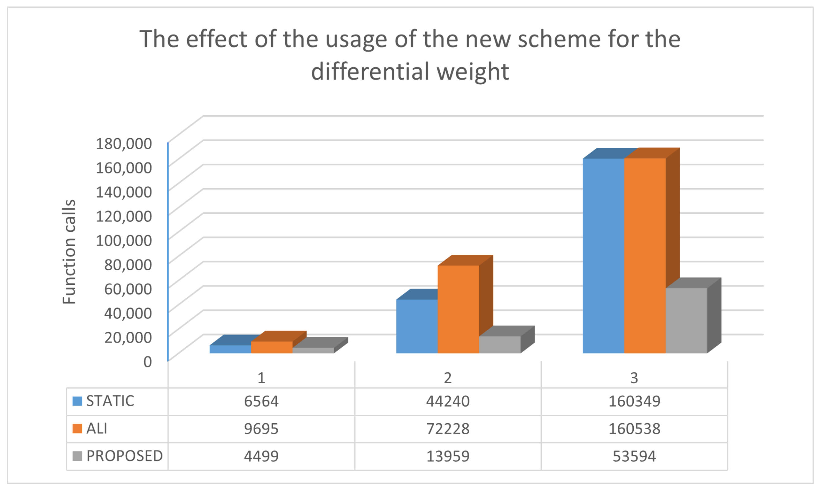
Figure 2.
Plot of function calls using the two modifications.
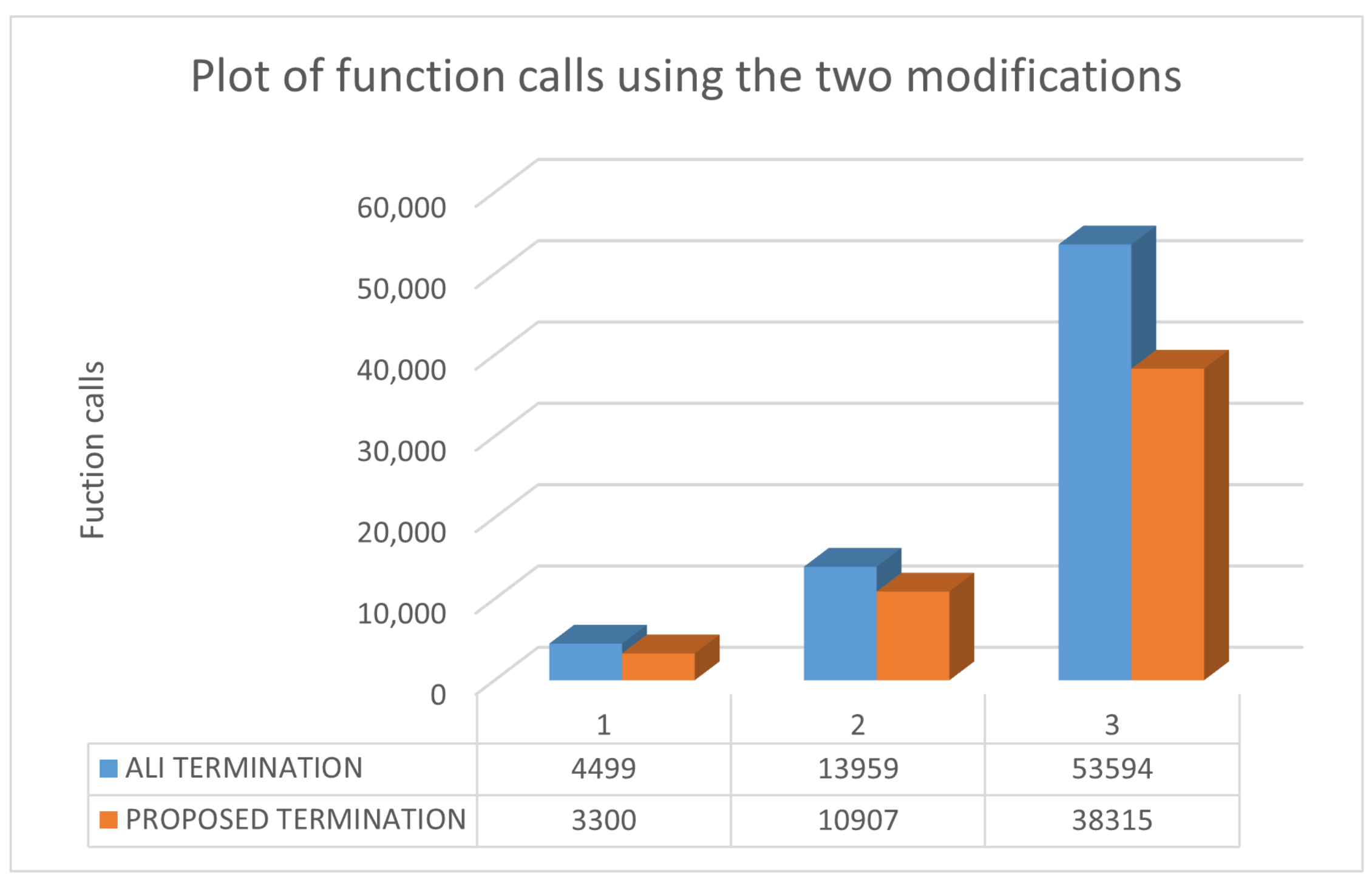
Figure 3.
Time comparisons for a variety of test functions.
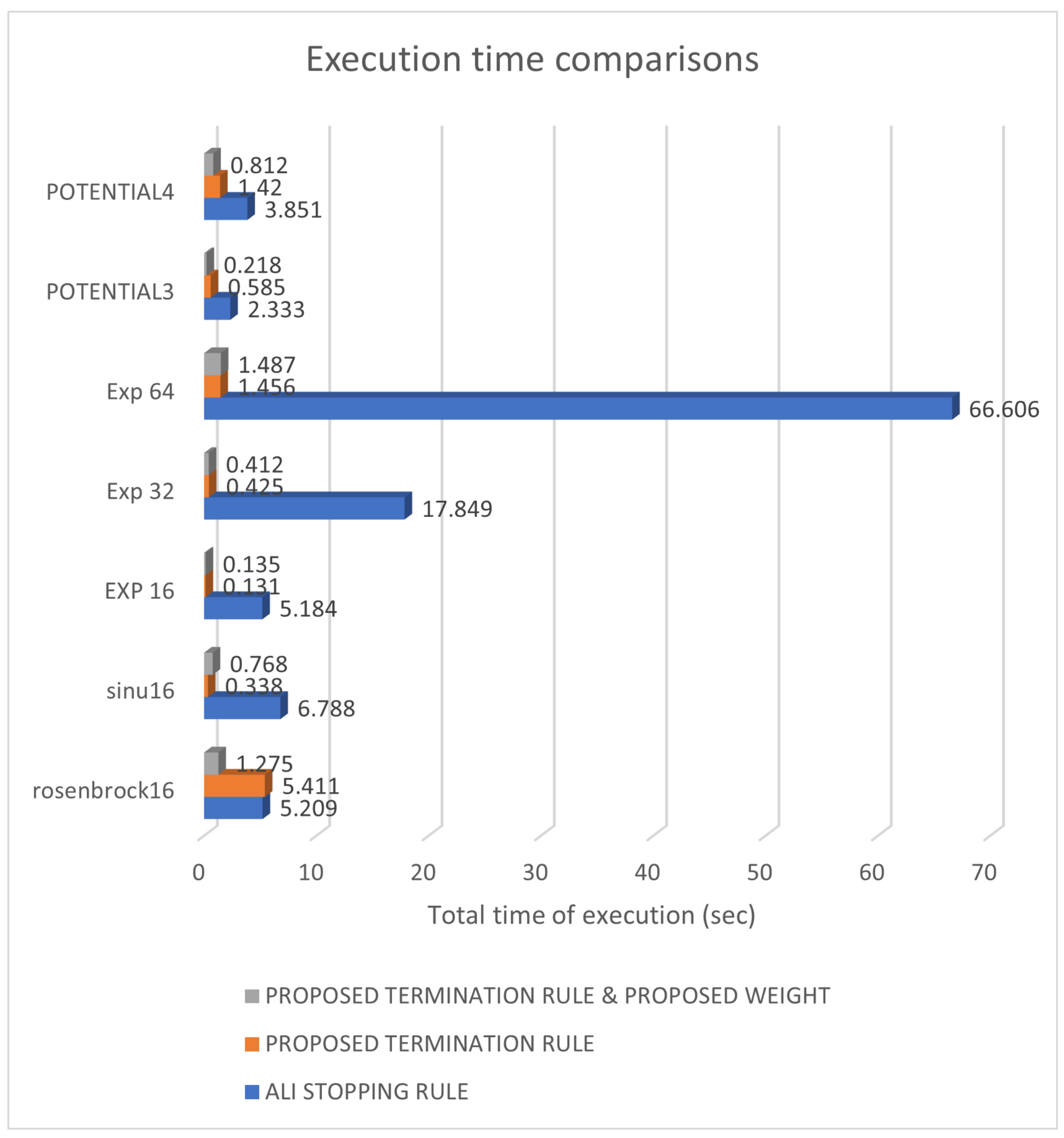
Figure 4.
Box plot representation and Wilcoxon rank-sum test results of the comparison among the schemes for the differential weights. The stopping rule used was that proposed by Ali in Equation (2). A p-value of less than 0.05 (2-tailed) was used for statistical significance and is marked with bold.


Table 1.
Experimental parameters.
| Parameter | Value |
|---|---|
| NP | 10n |
| F | 0.8 |
| CR | 0.9 |
| M | 20 |
Table 2.
Experiments with the termination rule of Ali.
| Function | Static | Ali | Proposed |
|---|---|---|---|
| BF1 | 1142 | 1431 | 847 |
| BF2 | 1164 | 1379 | 896 |
| BRANIN | 984 | 816 | 707 |
| CM4 | 3590 | 7572 | 2079 |
| CAMEL | 1094 | 18,849 | 685 |
| EASOM | 1707 | 2014 | 1327 |
| EXP2 | 532 | 323 | 449 |
| EXP4 | 2421 | 1019 | 1494 |
| EXP8 | 15,750 | 3670 | 5632 |
| EXP16 | 160,031 | 15,150 | 21,416 |
| EXP32 | 320,039 | 152,548 | 77,936 |
| GKLS250 | 784 | 944 | 614 |
| GKLS2100 | 772 | 1531 | 599 (0.97) |
| GKLS350 | 1906 (0.93) | 3263 | 1275 (0.93) |
| GKLS3100 | 1883 | 3539 | 1373 |
| GOLDSTEIN | 988 | 818 | 769 |
| GRIEWANK2 | 1299 (0.97) | 1403 | 883 (0.93) |
| HANSEN | 2398 | 2968 | 1400 |
| HARTMAN3 | 1448 | 836 | 1050 |
| HARTMAN6 | 9489(0.97) | 4015(0.97) | 4667(0.80) |
| POTENTIAL3 | 90,027 | 89,776 | 21,824 |
| POTENTIAL4 | 120,387 (0.97) | 120,405 (0.33) | 45,705 (0.97) |
| POTENTIAL5 | 150,073 | 150,104 | 83,342 |
| RASTRIGIN | 1246 | 1098 (0.93) | 871 |
| ROSENBROCK4 | 6564 | 9695 | 4499 |
| ROSENBROCK8 | 44,240 | 72,228 | 13,959 |
| ROSENBCROK16 | 160,349 (0.90) | 160,538 (0.60) | 53,594 |
| SHEKEL5 | 5524 | 3810 | 3057 (0.83) |
| SHEKEL7 | 5266 | 3558 | 2992 (0.87) |
| SHEKEL10 | 5319 | 3379 | 3076 |
| TEST2N4 | 4200 | 1980 | 2592 |
| TEST2N5 | 7357 | 2957 | 4055 |
| TEST2N6 | 12,074 | 4159 | 5836 |
| TEST2N7 | 18,872 | 5490 | 7904 |
| SINU4 | 3270 | 1855 | 2216 |
| SINU8 | 23,108 | 6995 | 8135 |
| SINU16 | 160,092 | 36,044 | 30,943 |
| SINU32 | 213,757 (0.70) | 160,536 (0.53) | 83,369 (0.80) |
| TEST30N3 | 1452 | 1732 | 959 |
| TEST30N4 | 1917 | 2287 | 1378 |
| Total | 1,564,515 (0.97) | 1,062,714 (0.96) | 506,404 (0.98) |
Table 3.
Experiments with the proposed termination rule.
| Function | Static | Ali | Proposed |
|---|---|---|---|
| BF1 | 996 | 1124 | 889 |
| BF2 | 926 | 1026 | 816 |
| BRANIN | 878 | 900 | 730 |
| CM4 | 1148 (0.70) | 1991 | 1103 |
| CAMEL | 1049 | 904 (0.93) | 846 |
| EASOM | 447 | 448 | 446 |
| EXP2 | 470 | 461 | 467 |
| EXP4 | 915 | 903 | 892 |
| EXP8 | 1797 | 3558 | 1796 |
| EXP16 | 3578 | 7082 | 3521 |
| EXP32 | 7082 | 14,125 | 7022 |
| GKLS250 | 498 | 576 | 493 |
| GKLS2100 | 533 | 884 (0.97) | 515 |
| GKLS350 | 823 | 1130 (0.93) | 814 (0.97) |
| GKLS3100 | 858 | 1495 (0.97) | 829 (0.93) |
| GOLDSTEIN | 945 | 993 | 915 |
| GRIEWANK2 | 947 | 921 | 826 |
| HANSEN | 2104 | 1949 | 1479 |
| HARTMAN3 | 1017 | 1005 | 952 |
| HARTMAN6 | 4679 (0.90) | 3744 (0.97) | 3128 (0.87) |
| POTENTIAL3 | 21,473 | 2284 | 8197 |
| POTENTIAL4 | 44,191 (0.43) | 3098 (0.33) | 24,659 (0.97) |
| POTENTIAL5 | 75,910 | 3443 | 52,664 |
| RASTRIGIN | 841 | 994 | 777 |
| ROSENBROCK4 | 4934 | 7192 | 3300 |
| ROSENBROCK8 | 29,583 | 49,696 | 10,907 |
| ROSENBCROK16 | 160,349 | 160,538 (0.60) | 38,315 |
| SHEKEL5 | 4389 (0.97) | 4266 | 2839 (0.83) |
| SHEKEL7 | 3905 | 3685 | 2668 |
| SHEKEL10 | 4049 | 3548 | 2629 |
| TEST2N4 | 2785 | 2275 | 2221 |
| TEST2N5 | 4481 | 3170 | 3122 |
| TEST2N6 | 6852 | 4286 | 4296 |
| TEST2N7 | 11971 | 5701 | 6267 |
| SINU4 | 2322 | 1987 | 1755 |
| SINU8 | 9990 | 6156 | 5113 |
| SINU16 | 6892 | 3628 (0.97) | 16,905 |
| SINU32 | 7235 (0.80) | 7438 (0.83) | 7218 |
| TEST30N3 | 1033 | 1098 | 951 |
| TEST30N4 | 1355 | 1444 | 1285 |
| Total | 432,610 (0.98) | 321,166 (0.96) | 224,567 (0.99) |
Publisher’s Note: MDPI stays neutral with regard to jurisdictional claims in published maps and institutional affiliations. |
© 2022 by the authors. Licensee MDPI, Basel, Switzerland. This article is an open access article distributed under the terms and conditions of the Creative Commons Attribution (CC BY) license (https://creativecommons.org/licenses/by/4.0/).
Share and Cite
MDPI and ACS Style
Charilogis, V.; Tsoulos, I.G.; Tzallas, A.; Karvounis, E. Modifications for the Differential Evolution Algorithm. Symmetry 2022, 14, 447. https://doi.org/10.3390/sym14030447
AMA Style
Charilogis V, Tsoulos IG, Tzallas A, Karvounis E. Modifications for the Differential Evolution Algorithm. Symmetry. 2022; 14(3):447. https://doi.org/10.3390/sym14030447
Chicago/Turabian StyleCharilogis, Vasileios, Ioannis G. Tsoulos, Alexandros Tzallas, and Evangelos Karvounis. 2022. "Modifications for the Differential Evolution Algorithm" Symmetry 14, no. 3: 447. https://doi.org/10.3390/sym14030447
Note that from the first issue of 2016, this journal uses article numbers instead of page numbers. See further details here.