Abstract
A multiresponse multipredictor semiparametric regression (MMSR) model is a combination of parametric and nonparametric regressions models with more than one predictor and response variables where there is correlation between responses. Due to this correlation we need to construct a symmetric weight matrix. This is one of the things that distinguishes it from the classical method, which uses a parametric regression approach. In this study, we theoretically developed a method of determining a confidence interval for parameters in a MMSR model based on a truncated spline, and investigating asymptotic properties of estimator for parameters in a MMSR model, especially consistency and asymptotic normality. The weighted least squares method was used to estimate the MMSR model. Next, we applied a pivotal quantity method, a Cramer–Wold theorem, and a Slutsky theorem to determine the confidence interval, investigate consistency, and asymptotic normality properties of estimator for parameters in a MMSR model. The obtained results were that the estimated regression function is linear to observation. We also obtained a confidence interval for parameters in the MMSR model, and the estimator for parameters in MMSR model was consistent and asymptotically normally distributed. In the future, these obtained results can be used as a theoretical basis in designing a standard toddlers growth chart to assess nutritional status.
1. Introduction
A regression model which is used to analyze the functional relationship between response variable and predictor variable in various fields is widely used for both prediction and interpretation purposes. This functional relationship is represented by a regression function. If we consider the form of the regression function, we recognize two types of regression models, namely a parametric regression (PR) model and a nonparametric regression (NR) model. The combination of the two types of regression models produces a semiparametric regression (SR) model. Furthermore, if this model has more than one predictor and response variables where there is a correlation between responses, the model is called a multiresponse multipredictor semiparametric regression (MMSR) model.
In general, the main problem in the regression modeling is estimation of the regression function. To estimate the regression function, there are several estimators which are frequently used in NR modeling; for example local linear, local polynomial, kernel, and spline. For prediction purposes, the use of local linear, local polynomial, and kernel estimators is highly recommended as discussed by [1,2,3,4,5,6,7,8,9,10,11]. Meanwhile, for prediction and interpretation purposes, the use of spline estimators is better and more flexible as discussed by [12,13,14]. Because of the flexible nature of this spline estimator, many researchers have been interested in using and developing it in several cases. For examples, an M-type spline estimator was discussed by [15]; truncated spline and B-spline estimators were discussed by [16,17], respectively; penalized spline has been proposed by [18] to analyze current status data. Additionally, spline smoothing has been proposed by [19] to estimate the regression function drawing the association between cortisol and ACTH hormones, and spline regression was proposed by [20] to estimate regression function applied to censored data. Next, [21,22] used both smoothing kernel and spline estimators to estimate the regression function and select the optimal smoothing parameter of uni-response nonparametric regression (UNR) models, and multiresponse nonparametric regression (MNR) models, respectively. A Kernel estimator was proposed by [23] to estimate UNR model through a simulation study. Additionally, [24] discussed kernel and spline smoothing techniques to estimate coefficient in a rates model. However, local linear, local polynomial and kernel estimators are highly dependent on the neighborhood of the target point, called the bandwidth, so that if used for model estimation of fluctuating data, a small bandwidth is required and this will result in an estimation curve that is too rough. So the estimators only consider the goodness of fit and do not consider smoothness. Thus, these estimators are not good to use for estimating models of fluctuating data in the sub intervals, because the estimation results will provide a large mean square error (MSE) value. This is different from the spline estimator which considers goodness of fit and smoothness factors as has been discussed by several researchers. Furthermore, [25] compared smoothing and truncated splines in a model for estimating blood pressures model, and the results showed that the smoothing spline is better at estimating the model than truncated spline, where it is shown by the MSE value if we use a smoothing spline estimator that is smaller than the truncated spline estimator. This means that for prediction purposes, the smoothing spline is better than the truncated spline. Additionally, [26] have discussed estimating a regression function in MNR model using smoothing spline and investigated asymptotic properties of the regression function. Application of smoothing spline and Fourier series was discussed by [27]. Although those researchers mentioned above have discussed several estimators to estimate the regression functions of the regression models, but those researchers discussed these estimators for UNR models and MNR models only. This means that those researchers mentioned above discussed estimators in NR models only.
Next, there are researchers who have discussed estimators in SR models; for examples [28,29] discussed smoothing techniques for estimating SR models; Ref. [30] used a spline estimator for determining the number of knots and their locations based on statistical criteria; Ref. [31] used an iterative weighted partial spline least squares estimator to estimate longitudinal SR model; Ref. [32] used a local linear estimator for designing the standard growth chart of children; Ref. [33] predicted GDP in Turkey using a SR model approach; Ref. [34] discussed a SR model applied to censored data; Refs. [35,36,37] discussed smoothing spline in SR models; Ref. [38] used bias-correction technique to construct the empirical likelihood ratios for estimating semiparametric model. However, those researchers discussed estimators in uni-response semiparametric regression (USR) models only. However, there are several researchers who have discussed estimators in a multiresponse semiparametric regression (MSR) model; for examples [39] studied estimating MSR using a smoothing spline estimator; Ref. [40] discussed determining confidence interval for the parameter of a parametric component of binary response SR model using truncated spline estimator; Ref. [41] discussed estimating the regression function and confidence interval of a parameter MSR model using a smoothing spline estimator. Furthermore, Ref. [42] discussed estimating the confidence interval for parameters of a MMSR model using a truncated spline estimator. However, all of the previous researchers mentioned above have not yet discussed determining consistency and asymptotic normality properties of parameters in a MMSR model by using truncated spline estimator.
In practice, we are often faced with the problem of analyzing the functional relationship between more than one response variable and more than one predictor variable where some of the response variables have a linear functional relationship with the response variable and some of the other predictor variables do not form a functional relationship that points to a certain pattern, and there is a correlation between responses. To deal with this problem, the MMSR model approach is used. Basically, the main goal of MMSR modeling is to get a better model than USR modeling, considering that this model not only considers the effect of predictors on responses, but also the relationship between responses. The representation of the relationship between responses is usually expressed in the form of a covariance matrix, which is used as a weighting in estimating the parameters of model. Hence, the problem of estimating the regression function is more complicated for a MMSR model, because the regression function in this model consists of a parametric component and a nonparametric component. Additionally, in this model there is a correlation between responses, so that in the estimation process the regression function requires a weight matrix in the form of a symmetric matrix, especially a diagonal matrix.
Therefore, in this article we discuss a new method for determining the confidence interval of parameters in the MMSR model and investigating asymptotic normality and consistency properties of parameters in the MMSR model based on a truncated spline estimator, which has a very good ability to handle data whose behavior changes (fluctuates) at certain sub-intervals.
2. Materials and Methods
In this section, we describe materials and methods which are used to determine asymptotic normality and consistency of parameters in the MMSR model based on truncated spline.
2.1. Multiresponse Multipredictor Semiparametric Regression (MMSR) Model
A paired observations set where ; ; ; represents response variable; and , and represent predictor variables follows a MMSR model if the relationship between observations of the response variable, namely , and observations of the predictor variables, namely , satisfies a model as follows:
where is the ith observation value in the kth response, is a parametric component of the kth response, is a nonparametric component of the kth response in which is assumed to be smooth in the sense that it fits in the Sobolev space , and is zero-mean random error with variance .
The multiresponse multipredictor semiparametric regression (MMSR) model presented by Equation (1) can be written as follows:
where is an unknown regression function of the MMSR model presented by Equation (1). This regression function consists of a parametric component and nonparametric component. Next, to estimate the regression function of the MMSR model presented by Equations (1) and (2) based on truncated spline estimator, we need to develop the truncated spline proposed by [12].
2.2. Truncated Spline
According to [12], the truncated section of a polynomial spline called as a piecewise polynomial, is a continuous segmented polynomial. A truncated spline regression model can adapt to the data characteristics, and it has the ability to overcome the data pattern showing a sharp rise or fall with the help of both knot points, and the number of knot points is such that its resulting curve is relatively smooth. Next, suppose we have a multiresponse multipredictor nonparametric regression (MMNR) model which can be expressed as follows:
Then, the truncated function with B knots (i.e., are knot points) and degree d is defined as follows [12]:
where d represents degree of polynomial in which generally for and , the Equation (4) gives the functions of linear polynomial, quadratic polynomial and cubic polynomial, respectively. Hence, based on Equations (3) and (4), the general form of truncated spline with degree of polynomial d and the number of knot points B for the regression function of MMNR model presented by Equation (3) can be expressed as follows:
Furthermore, we can develop this technique to the MMSR model for estimating the regression function of MMSR model presented by Equation (1) or Equation (2) based on truncated spline. Next, to determine the confidence interval for parameters in the MMSR model, we need the pivotal quantity method as proposed by [43].
2.3. Pivotal Quantity
Suppose we have a random sample of size n, ,,…,, of a population with probability density function where is an unknown parameter. If is a function of ,,…, and where its probability distribution is independent of the parameter , then is called a pivotal quantity [43].
Finally, based on the truncated spline estimator proposed by [12] and by applying weighted least square (WLS) method, we can estimate the MMSR model presented by Equation (1). Next, we apply development of pivotal quantity method proposed by [43] to determine confidence interval for parameters in MMSR model. Additionally, we investigate consistent property of estimator for parameters in MMS model, and then we apply Cramer–Wold theorem [44] and Slutsky theorem [45] to determine the asymptotic normality of estimator for parameters in the MMSR model presented by Equation (1).
2.4. Simulation
In this simulation we generated three samples sized . The response vector , consisting of three response variables and the design vector were produced from a uniform distribution. In addition, the MMSR model to be generated includes two different smooth functions, and with nonparametric covariates and , respectively. The number of replications for each sample used in simulation experiments were considered as 1000. Finally, the random error terms -s were independent and identically distributed from the multivariate normal distribution for three models.
3. Results and Discussions
The results and discussions presented in this section include estimating a MMSR model, estimating confidence interval of the parameters in a MMSR model, investigating the consistency of estimator for parameters in a MMSR model, determining asymptotic normality of estimator for parameters in a MMSR model, and simulation study.
3.1. Estimating MMSR Model
By considering Equations (4) and (5), the estimation of a MMSR model presented by Equation (1) or Equation (2) based on truncated spline estimator is approximated by a linear function that is in the form of truncated spline with degree of polynomial (i.e., a linear polynomial) and knot point b and the number of knots B such that the MMSR model presented by Equation (1) can be expressed as follows:
where and .
Therefore, the model presented by Equation (6) can be written in matrix notation as follows:
Next, let and then MMSR model presented by Equation (7) can be written as follows:
where ; ; ; .
Further, suppose is independently and identically distributed with zero mean and covariance (namely). Note that there is correlation between responses. This implies that there is correlation between random errors of each response variable, too. Therefore, for estimating parameters of the MMSR model we use the weighted least squares (WLS) method, which needs a symmetrical weight matrix that is the inverse of the covariance matrix . We can obtain construction of the covariance matrix as follows:
where ; .
Note that matrix , given in (9), is a symmetrical matrix. Next, based on assumptions of the MMSR model given in (1) that is zero-mean random error with variance , then it implies that and ; .
Hence, for we have:
Therefore, the matrix given in (9) can be written as follows:
where 0 is the null matrix, that is, a matrix in which all its element are null, and matrix is given as follows:
Estimation of parameters in the MMSR model presented by Equation (1) can be obtained by taking solution of the WLS optimization problem as follows:
Hence, by taking the partial derivative of with respect to as follows:
we get:
Next, based on the MMSR model presented in Equation (2) and the estimated parameters given by Equation (11), we have the estimated regression function of a MMSR model, namely , as follows:
Thus, by considering Equations (8), (11) and (12), we get an estimation of the MMSR model given by Equation (1) based on a truncated spline estimator as follows:
where
3.2. Estimating Confidence Interval of Parameters in MMSR Model
We assume that in the MMSR model presented by Equation (1) is normally distributed independently and identically with zero mean and variance . It is commonly written as where is unknown. Next, suppose we design the confidence interval for where ; and B is the number of knots. Therefore, we have a pivotal quantity as follows:
where ; ; and . The Equation (15) is pivotal quantity for parameter where is the element of the parameter vector , and is the diagonal element of . The pivotal quantity given by Equation (15) has a distribution of -student with a degree of freedom of .
Hereinafter, to determine the confidence interval for , we must take a solution of the following probability Equation:
where is the lower limit value of the confidence interval and is the upper limit value of the confidence interval, and is the confidence level.
Next, by substituting Equation (15) into Equation (16) we get:
Here, the Equation (17) can be written as follows:
where ; ; ; ; ; and subscript of in Equation (17) represents diagonal element of .
A confidence interval is called good if it has the shortest interval length. Because of this, we should determine values of and such that the length of the confidence interval in Equation (18) is the shortest.
Therefore, if represents the length of the confidence interval in Equation (18), then we have:
Hence, we must determine the solution of the following optimization problem to take the shortest length of confidence interval for :
and the following condition must be satisfied by Equation (19):
where function is a probability distribution of and function is a cumulative probability distribution of .
Next, by using a Lagrange multiplier method we have:
where is a Lagrange constant.
Hence, we get:
Based on Equations (22) and (23), we obtain:
The Equation (25) implies or . Since, in this case is not satisfied, then the shortest confidence interval for parameters vector must be taken from the values of and that satisfy the following Equation:
By using the confidence level , the values of and that satisfy Equation (26) can be found in table of distribution.
Hence, the shortest confidence interval for parameters of a MMSR model based on the truncated spline estimator satisfies the following probability:
where the value can be obtained from Equation (26) that is .
Therefore, we have:
Thus, by using -student distribution, the confidence interval for parameters vector of the MMSR model presented by Equation (1) based on the truncated spline estimator is:
where ; and B is the number of knots; ; ; ; subscript of represents the diagonal elements of matrix ; is a matrix of the predictor as given in Equation (8); and is a symmetrical covariance matrix as given in Equation (9).
3.3. Investigating Consistency of Estimator for Parameters in MMSR Model
Before investigating consistency of the estimator for parameters in the MMSR model namely , we need the following assumptions.
Assumption 1.
, and , ; .
Assumption 2.
, are independently and identically distributed with zero mean, the covariance matrix, and the third absolute moment is finite.
Assumption 3.
, .
For investigating consistent property of the estimator for the parameters of the MMSR model namely , we need the following Lemma 1 and Theorem 1.
Lemma 1.
Ifas presented in Equation (11) is a truncated spline estimator for the parameters of the multiresponse multipredictor semiparametric regression (MMSR) model, then
Proof of Lemma 1.
Based on Equations (8), and (11)–(14), we have:
Thus, we obtain:
□
Theorem 1.
If Assumptions 1–3 hold, then
Proof of Theorem 1.
Given matrices , , and ; ; Because Assumptions 1–3 hold, then:
- (a)
- Based on the Strong Law of Large Numbers [45], we have:it implies as .
- (b)
- Note that as hold if as .On the other hand, we have:It means that:Therefore, we obtain:□
Furthermore, the following Theorem provides a consistency property of that is a truncated spline estimator for parameters of MMSR model presented in Equation (1).
Theorem 2.
If is a truncated spline estimator for parameters of MMSR model presented in Equation (1), then
In other word, an estimatorthat satisfies the condition given in Equation (31) is said to be a consistent estimator.
Proof of Theorem 2.
Suppose is estimator as given in Equation (11). Based on Lemma 1 and Theorem 1, we get:
According to [45], for every we can express Equation (32) as follows:
Next, by using probability property, we get:
Thus, , . It means that is a consistent estimator. □
3.4. Determining Asymptotic Normality of Estimator for Parameters in MMSR Model
In this section, we determine asymptotic normality of that is a truncated spline estimator for parameters of the MMSR model presented in Equation (1). Before investigating asymptotic normality of , firstly we need to consider the following Lemma 2 and Theorem 3.
Lemma 2.
Ifis the matrix as given in Equation (14) and is the vector of the regression function of MMSR model, then
Proof of Lemma 2.
We have:
On the other hand, we have:
Hence, we obtain:
□
Theorem 3.
Ifis matrix as given in Equation (14) andis vector of regression function of MMSR model, then for n
Proof of Theorem 3.
To prove this theorem, we apply the Cramer–Wold theorem [44,45]. Given a vector such that:
where is the zero mean independent random variable. Therefore, has a mean of 0 and variance as follows:
Next, by taking into account the Assumptions 1–3, then converges to . Next, we have:
On the other hand, we obtain:
Due to Lemma 2 and finite third absolute moment of then converges to zero.
Thus, converges to a Normal distribution that is . □
Furthermore, the following Theorem provides asymptotic normality of that is a truncated spline estimator for parameters of the MMSR model presented in Equation (1). □
Theorem 4.
If is a truncated spline estimator of the parameters in the MMSR model presented in Equation (1), then for ,
Proof of Theorem 4.
By considering Equation (28), we can express as follows:
Hence, based on this we obtain:
as and as .
Furthermore, based on Theorem 3, we have:
Next, by applying Slutsky theorem [45], we obtain:
□
3.5. Simulation Study
In this section we give a simulation study for a MMSR model constructed by three response variables and three predictor variables.
- (i)
- Simulation Design: The simulation study scenarios are decided as follows:
- We generate three samples sized .
- The response vector , consisting of three response variables, is created from the MMSR model given in (ii).
- The design vector is produced from a uniform distribution.
- For each model, a total of nine regression coefficients specified as , are considered here.
- In addition, the MMSR model to be generated includes two different smooth functions, and with nonparametric covariates and , respectively.
- The number of replications for each sample used in simulation experiments is considered as 1000.
- (ii)
- Data Generation: The MMSR model can be written as follows, according to given information in the simulation design;where is a -dimensional design matrix and each is generated from a uniform distribution, that is, . The vector of regression coefficients is defined in (i) above.
- ▪
- and are computed by using and as follows:
- ▪
- Finally, the random error terms ’s are independent and identically distributed from the multivariate normal distribution for three models.
The results and comments regarding the simulation study are given in the following tables and figures below.
Table 1 contains the estimated regression coefficients for the parametric component of the MMSR model and their 95% confidence intervals. From this, it can be said that as the sample size increases, the confidence intervals narrow. Note that this inference is supported by the boxplots in Figure 1. In addition, it can be said that the proposed model has succeeded in obtaining satisfactory estimates for the parametric component.

Table 1.
Estimated regression coefficients from parametric component of the MMSR model.
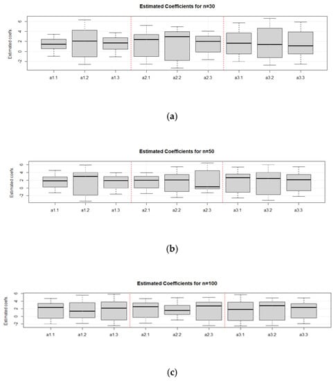
Figure 1.
Boxplots of estimated regression coefficients for all sample sizes. Note that a1.1, a1.2, and a1.3 seen on the x–axis of the boxplot show the regression coefficients obtained from the regression of . Similarly, a2.1, a2.2, and a2.3 show the coefficients from the
regression, while a3.1, a3.2, and a3.3 show the coefficients from the regression. (a). Boxplot of estimated regression coefficients for n = 30; (b). Boxplot of estimated regression coefficients for n = 50; (c). Boxplot of estimated regression coefficients for n = 100.
Figure 1 is drawn to see the convergence of the estimated regression coefficients to the true coefficients. It can be seen from the boxplots that, the range of the boxplot gets smaller as the sample sizes get larger. We would like to point out that this is an expected situation. Regarding the non-parametric component of the MMSR model, Table 2 and Figure 2 are obtained. Additionally, a Mann–Whitney U test is performed to determine the statistical significance of the difference between fitted curve and the real functions for both and , and the results are given in Table 2 below.
Table 2.
Results of Mann–Whitney U test for the nonparametric components.
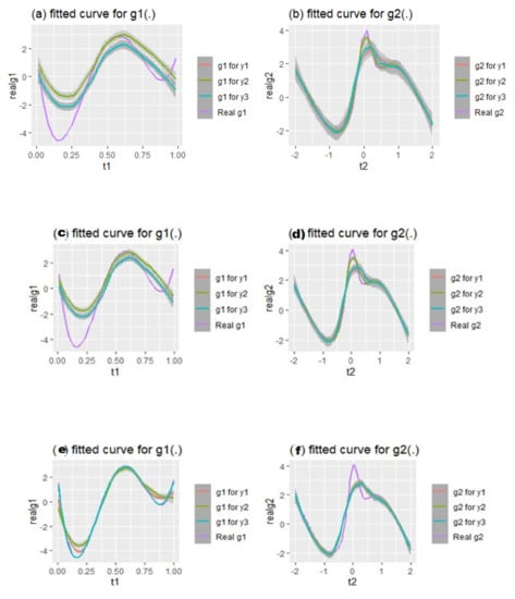
Figure 2.
Real functions and their fitted curves from the three MMSR models. (a,b) n = 30; (c,d) n = 50; (e,f) n = 100.
When the results given in Table 2 are examined carefully, it is seen that most of the p-Values are greater than 0.05 (these are shown in bold). As can be seen from this, it is clear that in most cases, the null hypothesis claiming that there is no difference between the medians of the fitted curves and the real functions cannot be rejected. In addition, these results are confirmed by the graphs given in Figure 2. Moreover, the influence of sample size is clearly visible from the panels in Figure 2.
After the parametric and nonparametric components, Figure 3 is obtained to examine the overall residuals from the total MMSR model. It should also be noted that Figure 3 includes the scatter plots for residuals versus fitted values of the MMSR model for all sample sizes. Note that although there is some improvement in the performance of the model when n = 100, it is clear that the residuals are not randomly distributed around zero. The existence of a heteroscedasticity problem is debatable. However, it has also been observed that when the sample size is large, the residuals do not exceed the standard deviation limits.
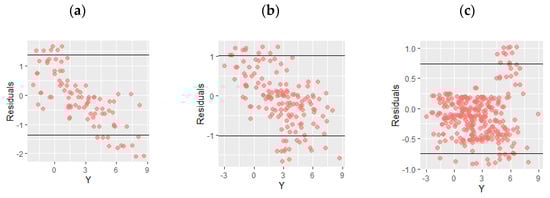
Figure 3.
Residual versus vector {i.e., } of the fitted response values. (a) n = 30; (b) n = 50; (c) n = 100.
4. Conclusions
The estimated MMSR model we obtained is a combination of estimations between the parametric and nonparametric components, and it is linear to observation. Additionally, we found that the confidence interval for parameters in a MMSR model depend on -student distribution namely and the estimator of parameters in a MMSR model is consistent and asymptotically normally distributed. Based on simulation results, the influence of sample size is clearly visible and it also has been observed that when the sample size is large, the residuals do not exceed the standard deviation limits.
Author Contributions
All authors have contributed to this research article, namely conceptualization, N.C., B.L.; methodology, B.L., N.C., I.N.B. and D.A.; software, D.A., N.C., T.S.; validation, B.L., N.C., I.N.B., T.S. and D.A.; formal analysis, B.L., N.C., I.N.B. and D.A.; investigation, resource and data curation, D.A., R.R., P.W. and A.A.; writing—original draft preparation, B.L. and N.C.; writing—review and editing, B.L., N.C. and D.A.; visualization, B.L., N.C. and D.A.; supervision, I.N.B., D.A., R.R., P.W. and A.A.; project administration, N.C. and B.L.; funding acquisition, N.C. All authors have read and agreed to the published version of the manuscript.
Funding
This research was funded by Airlangga University, the Republic of Indonesia through Mandated Research (Riset Mandat) Grant with grant number: 373/UN3.14/PT/2020.
Institutional Review Board Statement
Since this study does not involve humans and animals, then an Institutional Review Board Statement is not applicable.
Informed Consent Statement
Since this study does not involve humans, then Informed Consent Statement is not applicable.
Data Availability Statement
The authors confirm that there are no data available.
Acknowledgments
The authors thank Airlangga University for technical and financial support. The authors are also grateful to the editors and peer reviewers who provided comments, corrections, criticisms, and suggestions that were useful for improving the quality of this article.
Conflicts of Interest
The authors declare no conflict of interest. In addition, the funders had no role in the design of the study; in the collection, analyses, or interpretation of data; in the writing of the article, or in the decision to publish the results.
References
- Ana, E.; Chamidah, N.; Andriani, P.; Lestari, B. Modeling of hypertension risk factors using local linear of additive nonparametric logistic regression. J. Phys. Conf. Ser. 2019, 1397, 012067. [Google Scholar] [CrossRef]
- Cheruiyot, L.R. Local linear regression estimator on the boundary correction in nonparametric regression estimation. J. Statist. Theory Appl. 2020, 19, 460–471. [Google Scholar] [CrossRef]
- Chamidah, N.; Yonani, Y.S.; Ana, E.; Lestari, B. Identification the number of mycobacterium tuberculosis based on sputum image using local linear estimator. Bullet. Elect. Eng. Inform. (BEEI) 2020, 9, 2109–2116. [Google Scholar] [CrossRef]
- Cheng, M.-Y.; Huang, T.; Liu, P.; Peng, H. Bias reduction for nonparametric and semiparametric regression models. Statistica Sinica 2018, 28, 2749–2770. [Google Scholar] [CrossRef]
- Delaigle, A.; Fan, J.; Carroll, R.J. A design-adaptive local polynomial estimator for the errors-in-variables problem. J. Amer. Stat. Assoc. 2009, 104, 348–359. [Google Scholar] [CrossRef] [PubMed]
- Francisco-Fernandez, M.; Vilar-Fernandez, J.M. Local polynomial regression estimation with correlated errors. Comm. Statist. Theory Methods 2001, 30, 1271–1293. [Google Scholar] [CrossRef]
- Benhenni, K.; Degras, D. Local polynomial estimation of the mean function and its derivatives based on functional data and regular designs. ESAIM Probab. Stat. 2014, 18, 881–899. [Google Scholar] [CrossRef]
- Kikechi, C.B. On local polynomial regression estimators in finite populations. Int. J. Stats. Appl. Math. 2020, 5, 58–63. [Google Scholar]
- Wand, M.P.; Jones, M.C. Kernel Smoothing, 1st ed.; Chapman and Hall/CRC: New York, NY, USA, 1995. [Google Scholar]
- Cui, W.; Wei, M. Strong consistency of kernel regression estimate. Open J. Stats. 2013, 3, 179–182. [Google Scholar] [CrossRef]
- De Brabanter, K.; de Brabanter, J.; Suykens, J.A.K.; de Moor, B. Kernel regression in the presence of correlated errors. J. Mach. Learn. Res. 2011, 12, 1955–1976. [Google Scholar]
- Wahba, G. Spline Models for Observational Data; SIAM: Philadelphia, PA, USA, 1990. [Google Scholar]
- Eubank, R.L. Nonparametric Regression and Spline Smoothing, 2nd ed.; Marcel Dekker: New York, NY, USA, 1999. [Google Scholar]
- Wang, Y. Smoothing Splines: Methods and Applications; Taylor & Francis Group: Boca Raton, FL, USA, 2011. [Google Scholar]
- Liu, A.; Qin, L.; Staudenmayer, J. M-type smoothing spline ANOVA for correlated data. J. Multivar. Anal. 2010, 101, 2282–2296. [Google Scholar] [CrossRef]
- Chamidah, N.; Lestari, B.; Massaid, A.; Saifudin, T. Estimating mean arterial pressure affected by stress scores using spline nonparametric regression model approach. Commun. Math. Biol. Neurosci. 2020, 2020, 1–12. [Google Scholar]
- Eilers, P.H.C.; Marx, B.D. Flexible smoothing with B-splines and penalties. Statist. Sci. 1996, 11, 86–121. [Google Scholar] [CrossRef]
- Lu, M.; Liu, Y.; Li, C.-S. Efficient estimation of a linear transformation model for current status data via penalized splines. Stat. Meth. Medic. Res. 2020, 29, 3–14. [Google Scholar] [CrossRef]
- Wang, Y.; Guo, W.; Brown, M.B. Spline smoothing for bivariate data with applications to association between hormones. Stat. Sinica 2000, 10, 377–397. [Google Scholar]
- Yilmaz, E.; Ahmed, S.E.; Aydin, D. A-Spline regression for fitting a nonparametric regression function with censored data. Stats 2020, 3, 11. [Google Scholar] [CrossRef]
- Aydin, D. A comparison of the nonparametric regression models using smoothing spline and kernel regression. World Acad. Sci. Eng. Tech. 2007, 36, 253–257. [Google Scholar]
- Lestari, B.; Fatmawati; Budiantara, I.N.; Chamidah, N. Smoothing parameter selection method for multiresponse nonparametric regression model using spline and kernel estimators approaches. J. Phy. Conf. Ser. 2019, 1397, 012064. [Google Scholar] [CrossRef]
- Aydin, D.; Güneri, Ö.I.; Fit, A. Choice of bandwidth for nonparametric regression models using kernel smoothing: A simulation study. Int. J. Sci. Basic Appl. Research (IJSBAR) 2016, 26, 47–61. [Google Scholar]
- Osmani, F.; Hajizadeh, E.; Mansouri, P. Kernel and regression spline smoothing techniques to estimate coefficient in rates model and its application in psoriasis. Medic. J. Islamic Repub. Iran (MJIRI) 2019, 33, 90. [Google Scholar] [CrossRef]
- Fatmawati; Budiantara, I.N.; Lestari, B. Comparison of smoothing and truncated spline estimators in estimating blood pressures models. Int. J. Innov. Creat. Change (IJICC) 2019, 5, 1177–1199. [Google Scholar]
- Lestari, B.; Fatmawati; Budiantara, I.N. Spline estimator and its asymptotic properties in multiresponse nonparametric regression model. Songklanakarin J. Sci. Tech. (SJST) 2020, 42, 533–548. [Google Scholar]
- Mariati, M.P.A.M.; Budiantara, I.N.; Ratnasari, V. The application of mixed smoothing spline and Fourier series model in nonparametric regression. Symmetry 2021, 13, 2094. [Google Scholar] [CrossRef]
- Ruppert, D.; Wand, M.P.; Carroll, R.J. Semiparametric Regression; Cambridge University Press: New York, NY, USA, 2003. [Google Scholar]
- Heckman, N.E. Spline smoothing in a partly linear model. J. R. Stats. Soc. Ser. B. 1986, 48, 244–248. [Google Scholar] [CrossRef]
- Mohaisen, A.J.; Abdulhussein, A.M. Spline semiparametric regression models. J. Kufa Math. Comp. 2015, 2, 1–10. [Google Scholar]
- Sun, X.; You, J. Iterative weighted partial spline least squares estimation in semiparametric modeling of longitudinal data. Science in China Series A (Mathematics) 2003, 46, 724–735. [Google Scholar] [CrossRef]
- Chamidah, N.; Zaman, B.; Muniroh, L.; Lestari, B. Designing local standard growth charts of children in East Java province using a local linear estimator. Int. J. Innov. Creat. Change (IJICC) 2020, 13, 45–67. [Google Scholar]
- Aydin, D. Comparison of regression models based on nonparametric estimation techniques: Prediction of GDP in Turkey. Int. J. Math. Models Methods Appl. Sci. 2007, 1, 70–75. [Google Scholar]
- Aydın, D.; Ahmed, S.E.; Yılmaz, E. Estimation of semiparametric regression model with right-censored high-dimensional data. J. Stat. Comp. Simul. 2019, 89, 985–1004. [Google Scholar] [CrossRef]
- Gao, J.; Shi, P. M-Type smoothing splines in nonparametric and semiparametric regression models. Stat. Sinica 1997, 7, 1155–1169. [Google Scholar]
- Wang, Y.; Ke, C. Smoothing spline semiparametric nonlinear regression models. J. Comp. Graph. Stats. 2009, 18, 165–183. [Google Scholar] [CrossRef]
- Diana, R.; Budiantara, I.N.; Purhadi; Darmesto, S. Smoothing spline in semiparametric additive regression model with Bayesian approach. J. Math. Stats. 2013, 9, 161–168. [Google Scholar] [CrossRef][Green Version]
- Xue, L.; Xue, D. Empirical likelihood for semiparametric regression model with missing response data. J. Multivar. Anal. 2011, 102, 723–740. [Google Scholar] [CrossRef][Green Version]
- Wibowo, W.; Haryatmi, S.; Budiantara, I.N. On multiresponse semiparametric regression model. J. Math. Stats. 2012, 8, 489–499. [Google Scholar] [CrossRef]
- Li, J.; Zhang, C.; Doksum, K.A.; Nordheim, E.V. Simultaneous confidence intervals for semiparametric logistics regression and confidence regions for the multi-dimensional effective dose. Stat. Sinica 2010, 20, 637–659. [Google Scholar]
- Lestari, B.; Chamidah, N. Estimating regression function of multiresponse semiparametric regression model using smoothing spline. J. Southwest Jiaotong Univ. 2020, 55, 1–9. [Google Scholar]
- Hidayati, L.; Chamidah, N.; Budiantara, I.N. Confidence interval of multiresponse semiparametric regression model parameters using truncated spline. Int. J. Acad. Appl. Res. (IJAAR) 2020, 4, 14–18. [Google Scholar]
- Sahoo, P. Probability and Mathematical Statistics; University of Louisville: Lousville, KY, USA, 2013. [Google Scholar]
- Cramér, H.; Wold, H. Some theorems on distribution functions. J. London Math. Soc. 1936, 11, 290–295. [Google Scholar] [CrossRef]
- Sen, P.K.; Singer, J.M. Large Sample in Statistics: An Introduction with Applications; Chapman & Hall.: London, UK, 1993. [Google Scholar]


Publisher’s Note: MDPI stays neutral with regard to jurisdictional claims in published maps and institutional affiliations. |
© 2022 by the authors. Licensee MDPI, Basel, Switzerland. This article is an open access article distributed under the terms and conditions of the Creative Commons Attribution (CC BY) license (https://creativecommons.org/licenses/by/4.0/).