1. Introduction
Many problems in mathematics, physics or technics are modeled with the use of ordinary differential equations (ODEs) and the systems of such equations. However, these models are sometimes so complex that it is impossible to apply the analytical methods for solving them. In such cases, the only possibility lies in using some approximate methods. In this paper, we intend to compare three selected approaches dedicated for solving the ODEs. The first of them belong to the group of Runge–Kutta methods, very popular because of the ease of implementation and good speed of convergence of the obtained approximate solution. The most often used method, belonging to this family, is the classical Runge–Kutta method of order 4 (RK4), which is applied in the presented elaboration. This method is very popular and described in many sources; therefore, we omit here its detailed description. Instead, we recommend to the interested readers, for example, Ref. [
1]. Let us only recall that in order to solve the ODE task with the aid of the RK4 method, we need to present the problem in the form of equation
,
, with the initial condition
. Function
is the sought function, whereas
f is the given function of two variables, defined in some region
. In this method, we obtain the discrete approximate solution from the relation
where
is known from the initial condition,
, whereas
where
,
.
As the second way of solving the ODEs and their systems, we will use the routines available in the Mathematica software of version 12.2 (Mat), based on the implementation of selected methods and numerical treatment of differential equations. Thanks to the instruction DSolve, one can solve analytically the ODE and ODEs tasks, and by applying the instruction NDSolve, these kind of tasks can be solved numerically. We decided to use such an approach in order to confront the solutions calculated by the authors with the solutions delivered by a machine. The methods, built in Mathematica, can be applied for solving the ODE (ODEs) tasks, not necessarily defined in the normal form, as well as the equations of higher orders (with initial boundary conditions given in various forms).
The third method, applied for solving the ODEs tasks in this work, is the differential transformation method (DTM). This is the least known approach, which gives the reason to discuss this method more carefully in the next section. The main motivation of this paper is to show some kind of universality of the DTM method—this method can be applied for various forms of initial conditions and for various forms of the solved equation, including the implicit forms, and what is more, this method often leads to the exact solution of the problem, if it exists. Another essential, often unnoticeable, advantage is the following one: if the considered equation for the given initial conditions has no a unique solution (it has more than one solution), the DTM method very often finds all these solutions.
However, as with every method, the DTM method is not free from disadvantages. One of the disadvantages lies in the fact that the more complex problems, described by means of the more complex equations or their systems, require using the individual approach and constructing “manually” the proper formulas, with the aid of which will be possible to calculate the solution. Another one is the limitation of this method applicability to the equations, the components of which are the originals (explained in the next section); however, in real applications, this limitation has no important matter. The most important disadvantage of the DTM method seems to be the form of the sought solution—the solution is assumed in the form of a (function) power series, which may have a small convergence interval (in some extreme cases, it can be just one point).
Obviously, there exist many other methods, less known and less often applied, dedicated for solving ODEs tasks. Among them, we can specify the Adomian decomposition method [
2,
3], the homotopy perturbation method [
4] and many others.
2. Differential Transformation Method
Since the differential transformation method (DTM) is strictly connected with the expansion of a function into the Taylor series, we assume that we take into consideration only such functions, which can be expanded into the Maclaurin series (we can discuss the Maclaurin series, because the simple transformation
reduces the problem of expanding function
f into the Taylor series to the expansion of function
f into the Maclaurin series for variable
). Such functions are called “the originals”. So, if function
f is an original, then the following equality holds
which results directly from the theorem about the unique expansion of a function into the Maclaurin power series. This theorem states that any expansion of a function into the power series at point zero is equivalent to the expansion of this function into the Maclaurin power series.
Every original
f corresponds to function
F with nonnegative, integer arguments
k,
, according to the formula
Function F is called the T-function of function f, whereas the discussed transformation is called the Taylor transformation.
By having the
T-function
F, one can find the corresponding original in the form of its expansion into the Maclaurin series, according to the following formula
The Taylor transformation, introduced in [
5], possesses many useful properties. Some of them result directly from the form of the Maclaurin series of the given originals, while the others must be derived in more complicated way. The discussed properties are of great practical importance and make this tool quite simple to apply. In
Section 2.1, we present the properties of DTM, which will be used in the current elaboration. Proofs of these properties can be found, among others, in papers [
6,
7]. The authors of the current paper have also some achievements in this matter, which will be presented in detail in future papers. The DTM method quickly gained recognition and was used for many different problems, such as for solving ODE systems [
8], partial differential equations [
9], differential-algebraic equations [
7], selected types of equations, such as the Schrödinger equation [
10], Riccati equation [
11] or Bratu problem [
12], integral equations and integro-differential equations [
13,
14], fuzzy differential equations [
15], differential–difference equations [
16], fractional differential equations [
17]. The authors successfully used this method also in the calculus of variations, the difference equation, the difference–differential equation and various types of systems of the equations mentioned above (see, for example, the application of a similar method in [
18] for the systems of equations).
2.1. Properties of DTM
In all the investigated examples, we assume that the considered functions are the originals and that
If
then
If
then
If
then
If
then
If
then
If
then
If
,
then
If
then
If
,
,
, then
3. Initial Assumptions and Remarks
We investigate the differential equations of order
n (or the systems of such equations) possible to present in the form
where
is the sought function of variable
x,
F is the function of
variables defined in some region
. Many methods, including the RK method, require Equation (
12) to be presented in the normal form, which means the form of Equation (
12) that is possible to solve with respect to variable
:
This is quite a strong requirement since many nonlinear differential equations cannot be presented in the normal form; therefore, the applicability of the RK methods is significantly limited.
The next requirement for applicability of the RK methods is the form of conditions ensuring the uniqueness of solutions. The most frequent form is the form of the Cauchy problem in which the conditions are presented as follows
where
and
for
.
It happens, however, that we look for the solution of Equation (
12) by having the conditions written in the form
where
,
,
, or having the combination of conditions (
14) and (
15).
The next problem, which can be met while using the RK methods, concerns the differential equations of the higher orders. In a case when such a kind of equation cannot be presented in the normal form, it is possible sometimes to transform it into the system of n differential equations of the first order (the number of equations in the system is equal to the order of input equation).
4. Examples
In this section, we present a few selected examples, on the base of which we compare the investigated approaches.
4.1. Example 1
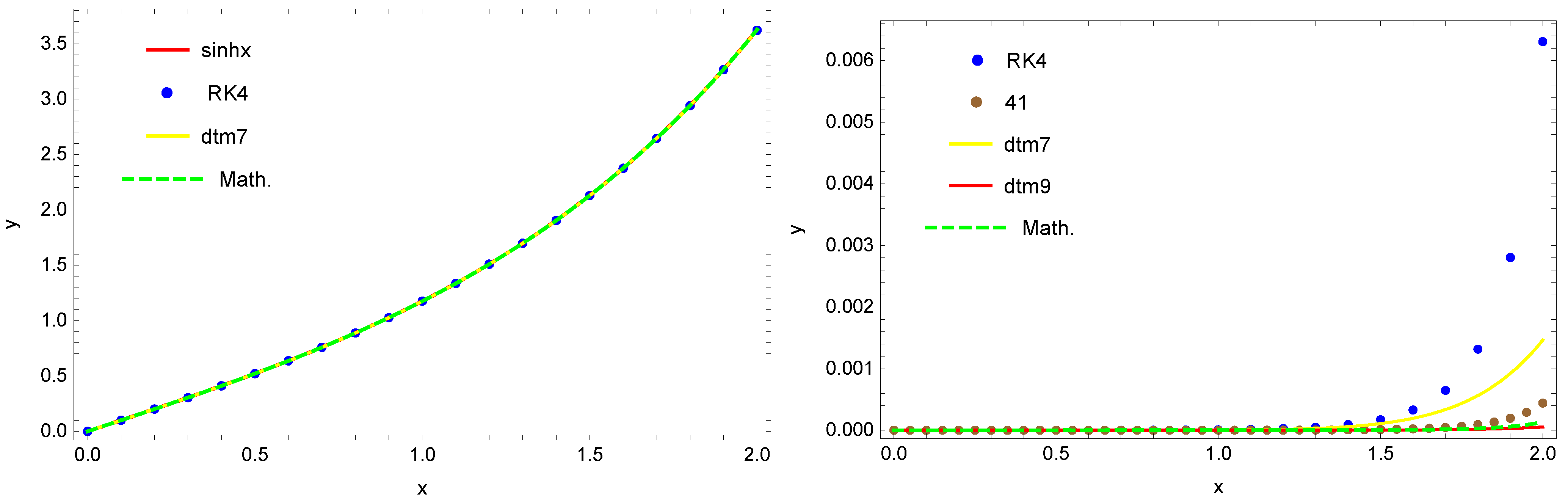
The first discussed equation is the Riccati equation of the following form
One can easy check that the solution of Equation (
16) is given by function
. Mathematica software finds the analytical form of the general solution of this equation, but it contains the integral that is impossible to determine, and therefore, such a solution is useless in practice. However, there is no trouble to obtain the numerical solution in the Mathematica software. Similarly easy is determining the approximate solution with the use of the RK4 method. By applying the DTM method for solving Equation (
16), we use the Taylor transformation. For this purpose, we apply, among others, Formulas (
3), (
6)–(
9), and we obtain the relation, given below, thanks to which we can determine recursively the values of the successive coefficients
for
:
From the initial condition, we have
and by substituting the successive values
to the relation (
17), we obtain in turn
Thanks to this, we can construct the following approximate solution based on eight components
or based on ten components as follows
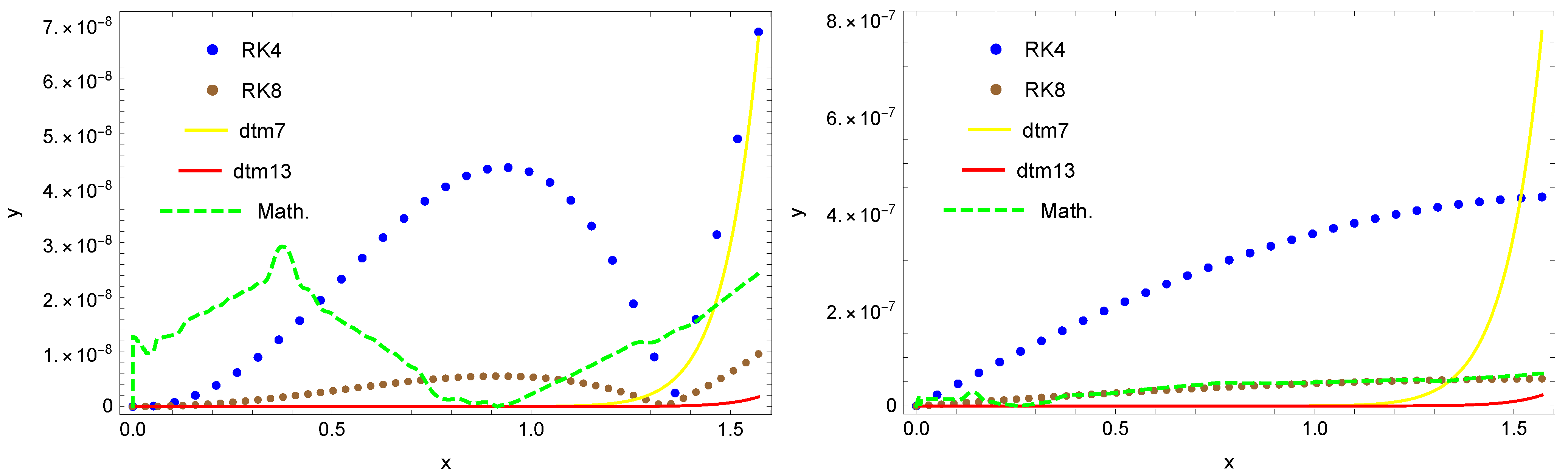
In
Figure 1, we present the comparison of solutions obtained with the aid of discussed methods together with the absolute errors
of the received approximations. In this figure, the solution obtained from the RK4 method with 21 discretization nodes is denoted by the blue dots and from the RK4 method with 41 discretization nodes denoted by brown dots. Solution (
18) is denoted by yellow line and solution (
19) by the red line, whereas the solution calculated in the Mathematica software is denoted by the green dashed line.
It is worth emphasizing that by using the DTM method, we obtain the exact values of the successive elements of the expansion of function into the Maclaurin series. Noting this fact, we can easily find the exact solution.
4.2. Example 2
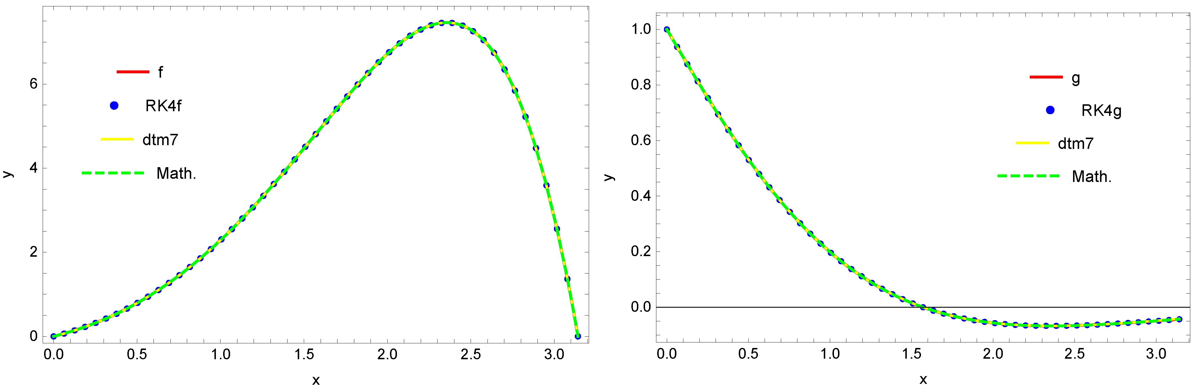
In the second example, we discuss the system of nonlinear differential equations which can be presented in the normal form
, with conditions
One can easily check that the exact solution of this system is represented by functions
It is worth noticing that this exact solution cannot be found by using the Mathematica software; however, there is no problem to obtain the approximate solution of the above defined system in this way.
Since the system (
20) is presented in the normal form, we can apply the RK4 method, but before we do that, we have to modify this method properly in order to adapt it to the systems of differential equations. In this case (in the case of systems with more equations, the modification is similar), we have (
and
are known from the initial condition (
21) and
):
where
,
. Thus, we obtain
for
.
Similar to the previous example, the greatest attention should be paid to the DTM method. This time, by using, among others, the properties (
3), (
4), (
6)–(
10), we transform the system (
20) with conditions (
21) into the following system for
:
where
Substituting the successive values
in the system (
22), we obtain
Generating in this way the successive values of
T-functions
and
,
, we can construct the approximate solution based on eleven components
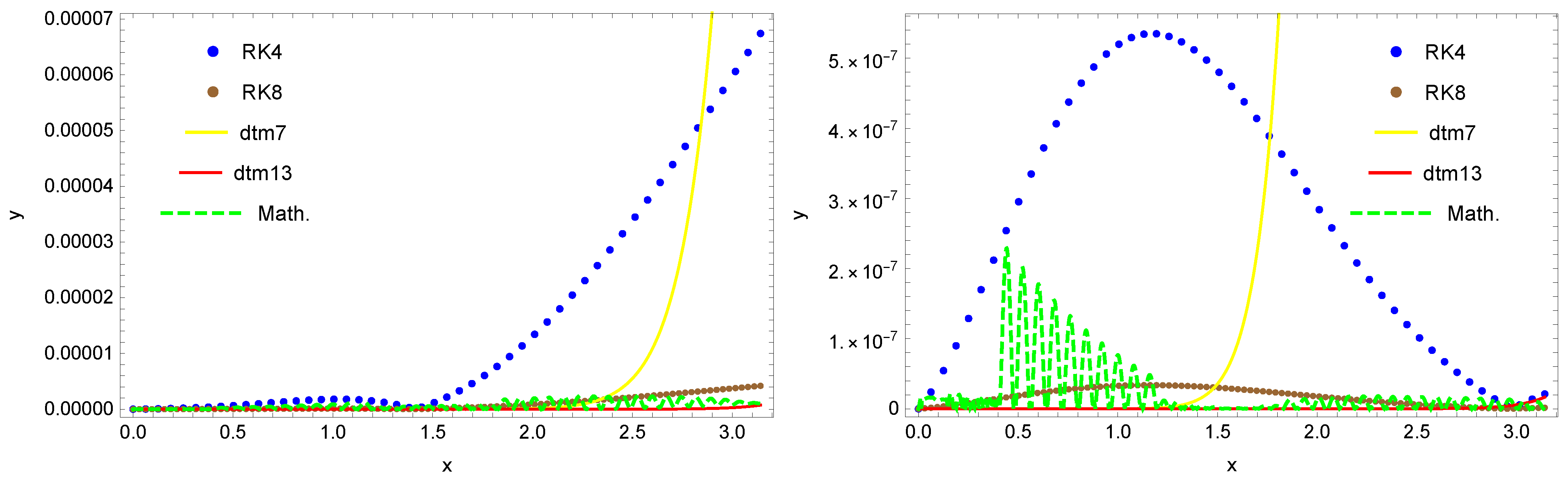
Figure 2 presents the comparison of solutions for functions
y (left figure) and
z (right figure) obtained by using all the discussed approaches, whereas
Figure 3 displays the absolute errors
of these approximate solutions for function
y (left figure) and
z (right figure). In the plots, the blue dots denote the solutions obtained by using the RK4 method with 51 discretization nodes, brown dots—by using RK4 method with 101 discretization nodes, yellow line—solutions
and
obtained by using the DTM method, red line—solutions
and
received by using the DTM method, and finally the green dashed line represents the solution calculated by applying the Mathematica software.
It should be emphasized that by applying the DTM method, we get the exact values of the successive elements of the expansions of functions
y and
z into the Maclaurin series. This time, however, it is not easy to notice what the analytical forms of these functions are. Therefore, we use the routine
FindGeneratingFunction, implemented in the Mathematica software, thanks to which we can obtain the exact solutions (
20) and (
21) of the investigated problem.
4.3. Example 3
In this example, we intend to find the solution of the initial problem described by the system of equations
for
with conditions
In order to apply the RK4 method for solving problems (
23) and (
24), we need to transform the discussed problem into the system of equations of the first order. Having the
n-order differential equation of the form
for
, with conditions
we can introduce new variables
thanks to which the given equation can be written in the form of the system of the first-order differential equations, as follows
with conditions
By acting in this way, we transform problems (
23) and (
24) into the form of the system of four differential equations of the first order, and next, similar to example
4.2, we adapt the formulas describing the RK4 method to the dimension of the task.
Again, similar to the previous examples, Mathematica software is not able to give the solution of the investigated problem in the analytical form, but it can easily give the approximate solution.
Solving this problem with the aid of the DTM method, we assume that the functions
Y and
Z represent the images of functions
y and
z. Basing on the properties (
4)–(
7) and (
9), we obtain the following system of equations from the system of Equations (
23) and conditions (
24), for
:
where
Substituting in the system (
25) the successive values
, we obtain
Generating in this way the successive values of
T-functions
and
, for
, and applying next, once again, the routine
FindGeneratingFunction, built in the Mathematica software, we receive the exact solution of the examined problem
Correctness of this result can be easily verified.
In
Figure 4, we show the comparison of solutions for functions
y (left figure) and
z (right figure) obtained by using all the examined approaches, whereas
Figure 5 presents the absolute errors
of these approximate solutions for function
y (left figure) and
z (right figure). In the plots, the blue dots denote the solutions obtained by using the RK4 method with 51 discretization nodes, brown dots—by using the RK4 method with 101 discretization nodes, yellow line—solutions
and
received by using the DTM method, red line—solutions
and
obtained by using the DTM method, and finally the green dashed line represents the approximate solution given by the Mathematica software.
4.4. Example 4
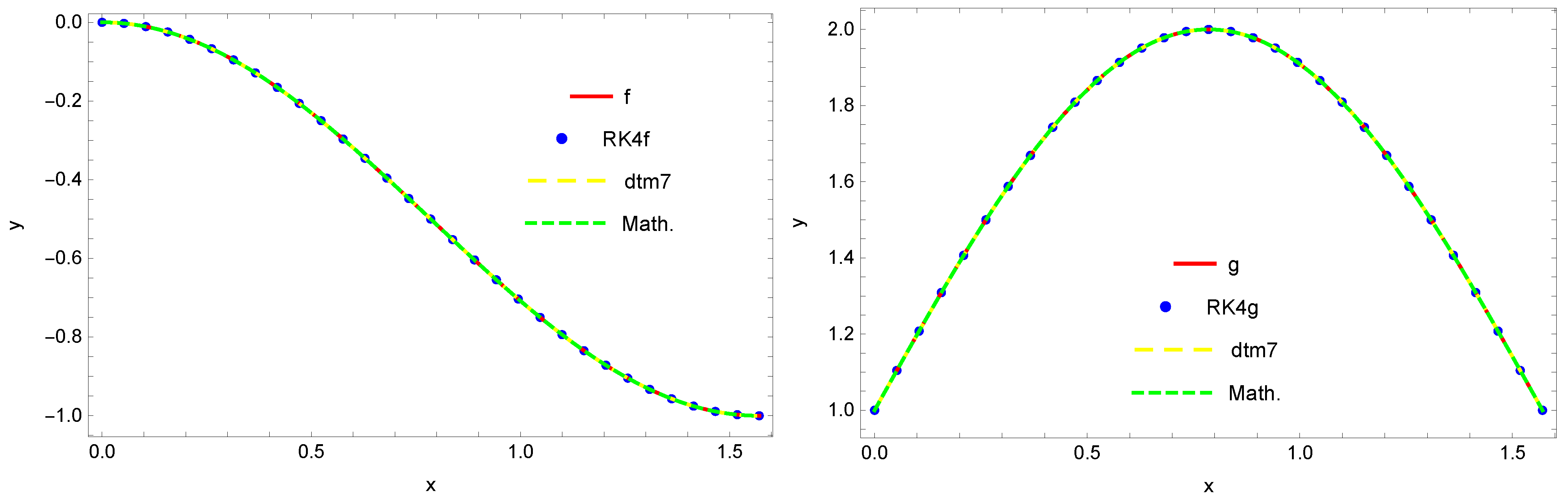
As the next example, in this section, we consider the system of differential equations with the boundary conditions, different from the previous example when the system is completed by the initial conditions.
So, we have the system of differential equations
with boundary conditions of the first kind
Because of the form of conditions (
27), this problem cannot be solved by means of the RK4 method. It is possible to solve this problem by applying the Mathematica software, no matter the form of conditions (
27). In this case, like in the previous examples, the useful analytical solution cannot be found, but there is no problem with obtaining the approximate solution.
In order to use the DTM method, we need to notice that we do not know the values of the first-order derivatives of functions
y and
z for
. Therefore, we assume temporarily that
and
. Hence, and from the half of conditions (
27), we obtain
If we assume that functions
and
are the images of functions
and
, respectively, then from Equation (
27), on the basis of properties (
3), (
4), (
6)–(
9), we receive the following relations for
Assuming that we determine five successive components from the above relations, that is, by taking , we obtain
- —for :
- — for :
- — for :
- — for :
- — for :
Thus we have the approximate solution
depending on the unknown parameters
and
. To determine their values we need to use the other half of the defined boundary conditions and solve the system of equations
It appears that three solutions of this systems exist:
In order to select the best one from among these solutions, we construct three groups of the approximate solutions,
,
, and
, and we examine the errors of these solutions,
,
, for
, where
means the right-hand sides of the system (
26) of equations.
We can observe that the best solution is the one provided by the third pair of parameters.
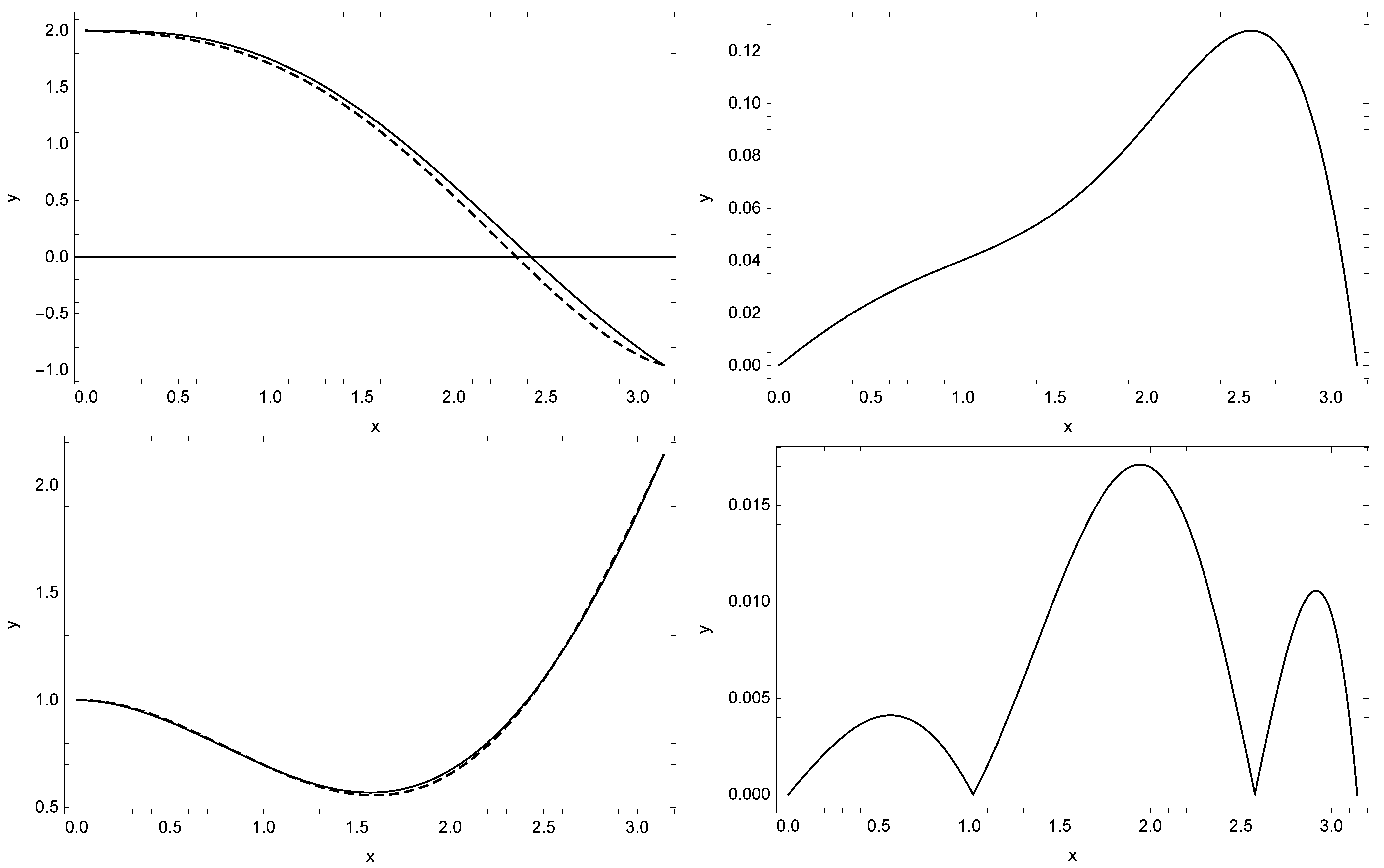
Figure 6 shows the exact solution and the approximate solution
,
received for the selected pair of parameters together with the errors of these approximations.
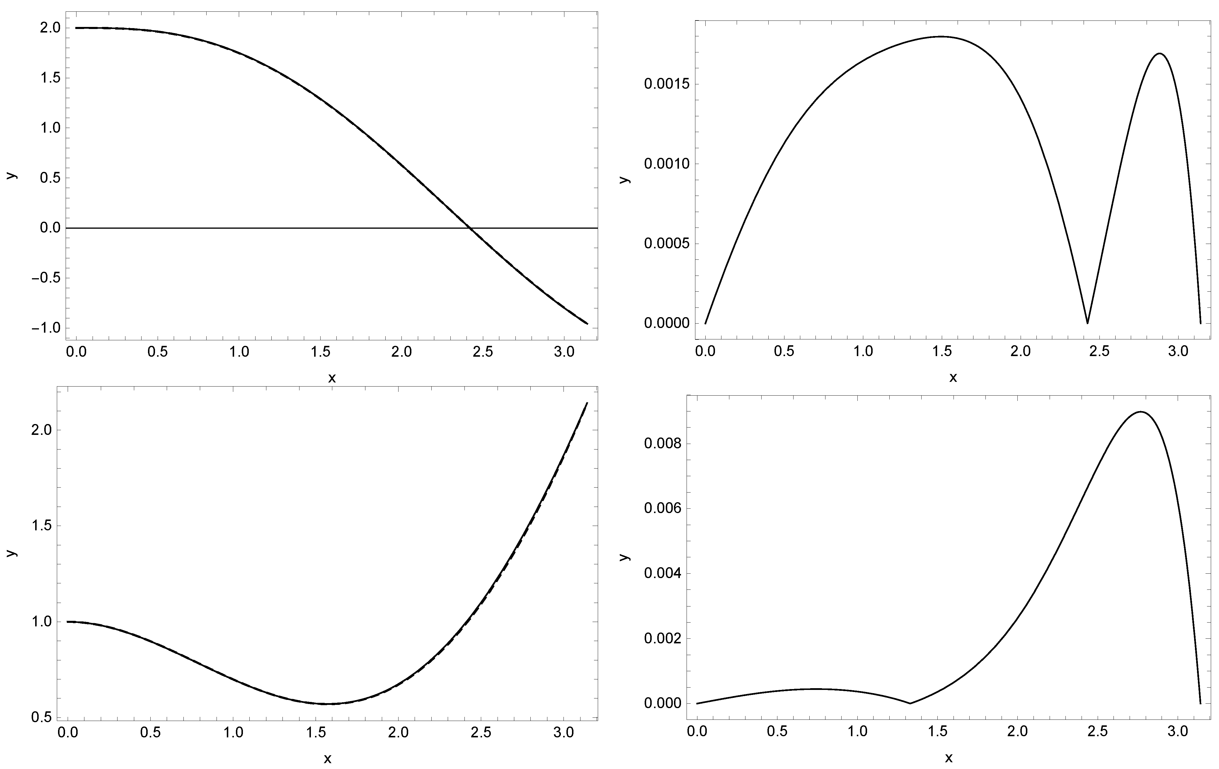
If we increase the number of the determined components and create in this way the approximate solution
,
, then we obtain the result displayed in
Figure 7 (in this case, we have five groups of solutions and the best one is for
and
—chosen in the same way as described above).
Figure 6 and
Figure 7 could be made on the basis of the known exact solutions, which are the functions
whereas the parameters
and
then take the values
.
4.5. Example 5
As the last example in this section, let us consider the following differential equation
with condition
Equation (
28) cannot be solved by using the RK method (this equation cannot be presented in the normal form). Mathematica software is also helpless in this case (even the approximate solution cannot be found).
The last hope is the DTM method. In order to apply the DTM method, let us assume that function
is the image of function
. Then, from Equation (
28), basing, among others, on properties (
3) and (
6)–(
10), we obtain for
- — for :
- — for :
- — for :
Solving the equations, described by means of relation (
30), for the successive values
, we obtain the sought values
for
:
On this ground, we can suppose that
Hence we are able to predict the solution of problem (
28):
The above function is in fact the exact solution of task (
28), which can be easily verified.
5. Conclusions
In the paper, we have presented the comparison of three approaches used for solving ordinary differential equations of any order, as well as the systems of such equations. The main goal of this elaboration was to indicate and justify the advantages of the differential transformation method (DTM), which is less known and not often applied. For this purpose, we investigated this method on the background of two other popular methods: the Runge–Kutta method (we decided to use the Runge–Kutta method of order 4 to emphasize better the advantages of the DTM method) and the methods built in the Mathematica software (the discussed examples and the figures illustrating the obtained solutions were realized in version 12.2 of the Mathematica program). The choice of these methods was dictated by their popularity (considering especially the RK4 method) or their simplicity—Mathematica software offers the special routines dedicated for solving the differential equations and their systems, based on the implementation of selected methods and numerical treatment of differential equations. The offered routines are the obvious and default tools for Mathematica users. It is worth mentioning that one does not need to purchase the license for using Mathematica because the tools of this software are available freely on the web page
https://www.wolframalpha.com (last access date: 18 December 2021).
The exemplary problems, presented in this paper, were not accidentally chosen. The examples describe the problems that are possible to solve by using all the three discussed approaches (Examples 1–3), impossible to solve by using the RK4 method (Example 4—because of the form of conditions; and Example 5—because of the implicit form of the equation) and impossible to solve with the aid of the Mathematica program (Example 5). Despite these problems, all the presented examples could be successfully solved by applying DTM method which shows universality of this method—this method can be used for various forms of initial conditions and for various forms of the solved equation, including the implicit forms. Moreover, the errors of approximate solutions, obtained in the DTM method, are comparable, or very often even lower, than the errors generated by the other methods. What is more and worth emphasizing, the DTM method often leads to the exact solution of the problem, if it exists.
The usefulness of the DTM method, shown in this paper, encourages undertaking a further study on some other applications of this method. At present, the authors are investigating the possibility of applying the discussed method for solving the differential–integral–algebraic equations and the integral equations with retarded argument. Many interesting and important problems are also described by means of the fractional differential equations (see for example [
19,
20]), possible to solve by applying the DTM method as well.
Author Contributions
Conceptualization, M.P.; methodology, E.H. and M.P.; software, M.P.; validation, E.H. and M.P.; formal analysis, E.H. and M.P.; investigation, E.H. and M.P.; data curation, M.P.; writing—original draft preparation, E.H.; writing—review and editing, E.H.; visualization, M.P.; supervision, E.H. and M.P.; project administration, E.H. and M.P. All authors have read and agreed to the published version of the manuscript.
Funding
This research received no external funding.
Institutional Review Board Statement
Not applicable.
Informed Consent Statement
Not applicable.
Data Availability Statement
Not applicable.
Conflicts of Interest
The authors declare no conflict of interest. The funders had no role in the design of the study; in the collection, analyses, or interpretation of data; in the writing of the manuscript; or in the decision to publish the results.
References
- Gautschi, W. Numerical Analysis, 2nd ed.; Springer Science & Business Media: Boston, MA, USA, 2012. [Google Scholar]
- Adomian, G. Solving Frontier Problems of Physics: The Decomposition Method; Kluwer: Dordrecht, The Netherlands, 1994. [Google Scholar]
- Hetmaniok, E.; Słota, D.; Wituła, R.; Zielonka, A. Comparison of the Adomian decomposition method and the variational iteration method in solving the moving boundary problem. Comput. Math. Appl. 2011, 61, 1931–1934. [Google Scholar] [CrossRef]
- Hetmaniok, E.; Nowak, I.; Słota, D.; Zielonka, A. Solution of the Inverse Heat Conduction Problem with Neumann Boundary Condition by Using the Homotopy Perturbation Method. Therm. Sci. 2013, 17, 643–650. [Google Scholar] [CrossRef]
- Zhou, J.K. Differential Transformation and Its Application for Electrical Circuits; Huarjung University Press: Wuhan, China, 1986. [Google Scholar]
- Arikoglu, A.; Özkol, I. Solution of boundary value problems for integrodifferential equations by using differential transform method. Appl. Math. Comput. 2005, 168, 1145–1158. [Google Scholar]
- Ayaz, F. On the Two-Dimensional Differential Transform Method. Appl. Math. Comput. 2003, 143, 361–374. [Google Scholar] [CrossRef]
- Mirzaee, F. Differential Transform Method for Solving Linear and Nonlinear Systems Ordinary Differential Equations. Appl. Math. Sci. 2011, 5, 3465–3472. [Google Scholar]
- Ayaz, F. Solutions of the System Partial Differential Equations by Differential Transform Method. Appl. Math. Comput. 2004, 147, 547–567. [Google Scholar]
- Kanth, R.; Aruna, K. Two-dimensional differential transform method for solving linear and non-linear Schrödinger equations. Chaos Solitons Fractals 2009, 41, 2277–2281. [Google Scholar] [CrossRef]
- Mukherjee, S.; Roy, B. Solution of Riccati Equation with Variable Co-efficient by Differential Transform Method. Int. J. Nonlinear Sci. 2012, 14, 251–256. [Google Scholar]
- Abdel-Halim Hassan, I.H.; Erturk, V.S. Applying Differential Transformation Method to the One-Dimensional Planar Bratu Problem. Int. J. Contemp. Math. Sci. 2007, 2, 1493–1504. [Google Scholar] [CrossRef]
- Celik, E.; Tabatabaei, K. Solving a Class of Volterra Integral Equation Systems by the Differential Transform Method. Int. J. Nonlinear Sci. 2013, 16, 87–91. [Google Scholar]
- Biazar, J.; Eslami, M.; Islam, M.R. Differential Transform Method for Special Systems of Integral Equations. J. King Saud Univ. Sci. 2012, 24, 211–214. [Google Scholar] [CrossRef]
- Allahviranloo, T.; Kiani, N.A.; Motamedi, N. Solving fuzzy differential equations by differential transformation method. Inf. Sci. 2009, 179, 956–966. [Google Scholar] [CrossRef]
- Liu, B.; Zhou, X.; Du, Q. Differential Transform Method for Some Delay Differential Equations. Appl. Math. 2015, 6, 585–593. [Google Scholar] [CrossRef]
- Arikoglu, A.; Özkol, I. Solution of fractional differential equations by using differential transform method. Chaos Solitons Fractals 2007, 34, 1473–1481. [Google Scholar] [CrossRef]
- Grzymkowski, R.; Pleszczyński, M. Application of the Taylor transformation to the systems of ordinary differential equations. In Information and Software Technologies 2018, ICIST; Damaševičius, R., Vasiljeviene, G., Eds.; Springer: Cham, Switzerland, 2018; Volume 920, pp. 379–387. [Google Scholar] [CrossRef]
- Jafari, H.; Ganji, R.M.; Nkomo, N.S.; Lv, Y.P. A numerical study of fractional order population dynamics model. Results Phys. 2021, 27, 104456. [Google Scholar] [CrossRef]
- Ganji, R.M.; Jafari, H.; Moshokoa, S.P.; Nkomo, N.S. A mathematical model and numerical solution for brain tumor derived using fractional operator. Results Phys. 2021, 28, 104671. [Google Scholar] [CrossRef]
| Publisher’s Note: MDPI stays neutral with regard to jurisdictional claims in published maps and institutional affiliations. |
© 2022 by the authors. Licensee MDPI, Basel, Switzerland. This article is an open access article distributed under the terms and conditions of the Creative Commons Attribution (CC BY) license (https://creativecommons.org/licenses/by/4.0/).


