Introduction
Current methods for monitoring sites contaminated with volatile organic compounds (VOCs) often employ manual grab samples with off-site laboratory analysis that are extremely costly and time- consuming. The integrity of these off-site analyses can be compromised during sample collection, transport, and storage. An attractive alternative is the use of real-time sensors that can be placed in situ, which may reduce the need for manual samples and expensive off-site analyses. While technologies exists to detect and analyze volatile organic compounds (VOCs), very few systems are designed to be deployed in situ (e.g., in soil and water) while providing real-time, continuous, long-term monitoring. Many of these existing technologies (e.g., gas chromatography, photoionization) include sensitive electronic components and require the flow of a carrier gas during operation, which may not be amenable to long-term in-situ monitoring applications.
The purpose of this work is to develop simple, rugged,
in-situ microchemical sensors and systems that can be used to provide unattended real-time monitoring and characterization of VOCs (e.g., trichloroethylene) in soil and groundwater. The intent is to reduce costs associated with monitoring sites contaminated with VOCs and to improve public and stakeholder confidence in the long-term stewardship of contaminated sites through the use of continuous
in-situ monitoring systems. The technology for these devices can also be used in other arenas where volatile organic compounds need to be monitored continuously
in situ (e.g., Homeland Security, process monitoring, worker safety, etc.). This paper focuses on the development of a surface acoustic wave (SAW) sensor system that can be deployed in geologic environments. Previous studies by Frye [
1] have investigated the use of SAW sensors for detecting volatile organic compounds
in situ. However, the system developed by Frye [
1] requires the use of a carrier gas to collect and pass the sample over the sensor. In addition, their system can only be used for gas-phase sampling. This work integrates an array of SAW sensors with a unique packaging design [
2] to allow the SAW sensor to operative passively (no carrier gas) in a variety of media (air, soil, or water).
Principles of Surface Acoustic Wave Sensor
Surface-acoustic-wave (SAW) sensors consist of an input transducer, a chemically adsorbent polymer film, and an output transducer on a peizoelectric substrate, which is typically quartz. The input transducer launches an acoustic wave that travels through the chemical film and is detected by the output transducer. The Sandia-made device runs at a very high frequency (approximately 525 MHz), and the velocity and attenuation of the signal are sensitive to the viscoelasticity and mass of the thin film [
3]. SAWS have been able to distinguish organophosphates, chlorinated hydrocarbons, ketones, alcohols, aromatic hydrocarbons, saturated hydrocarbons, and water [
4].
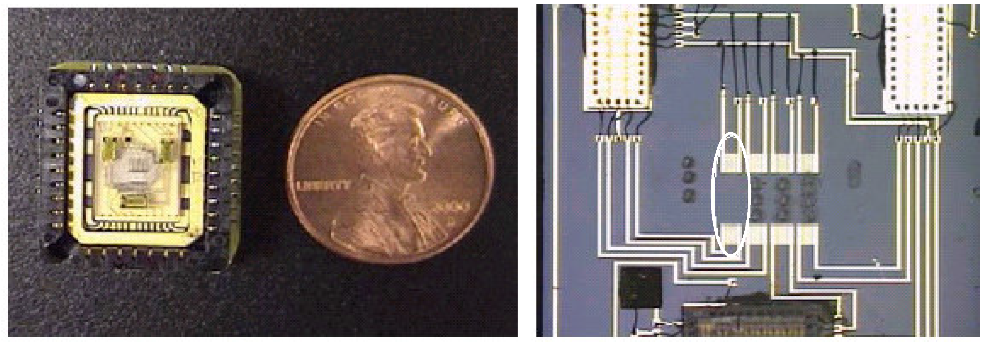
The SAW used in these tests have four channels—each channel consists of a transmitter and a receiver, separated by a small distance. Three of the four channels have a polymer deposited on the substrate between the transmitter and receiver (
Figure 1). The purpose of the polymers is to adsorb chemicals of interest, with different polymers having different affinities to various chemicals. When a chemical is adsorbed, the mass of the polymer increases, causing a slight change in phase of the acoustic signal relative to the reference (fourth) channel, which does not contain a polymer. The SAW device also contains three Application Specific Integrated Circuit chips (ASICs), which contain the electronics to analyze the signals and provide a DC voltage signal proportional to the phase shift. The SAW device, containing the transducers and ASICs, is bonded to a piece of quartz glass, which is placed in a leadless chip carrier (LCC) (see
Figure 1). Wire bonds connect the terminals of the leadless chip carrier to the SAW circuits.
Packaging for In-Situ Operation
A rugged package was designed for the SAW sensor to allow it to be used in subsurface environments. The design of the SAW sensor housing was modeled after the chemiresistor assembly developed by Ho and Hughes [
2]. The primary difference between the chemiresistor housing and the SAW housing is that the outer collar for the SAW sensor is longer to accommodate additional electronics on a circuit board.
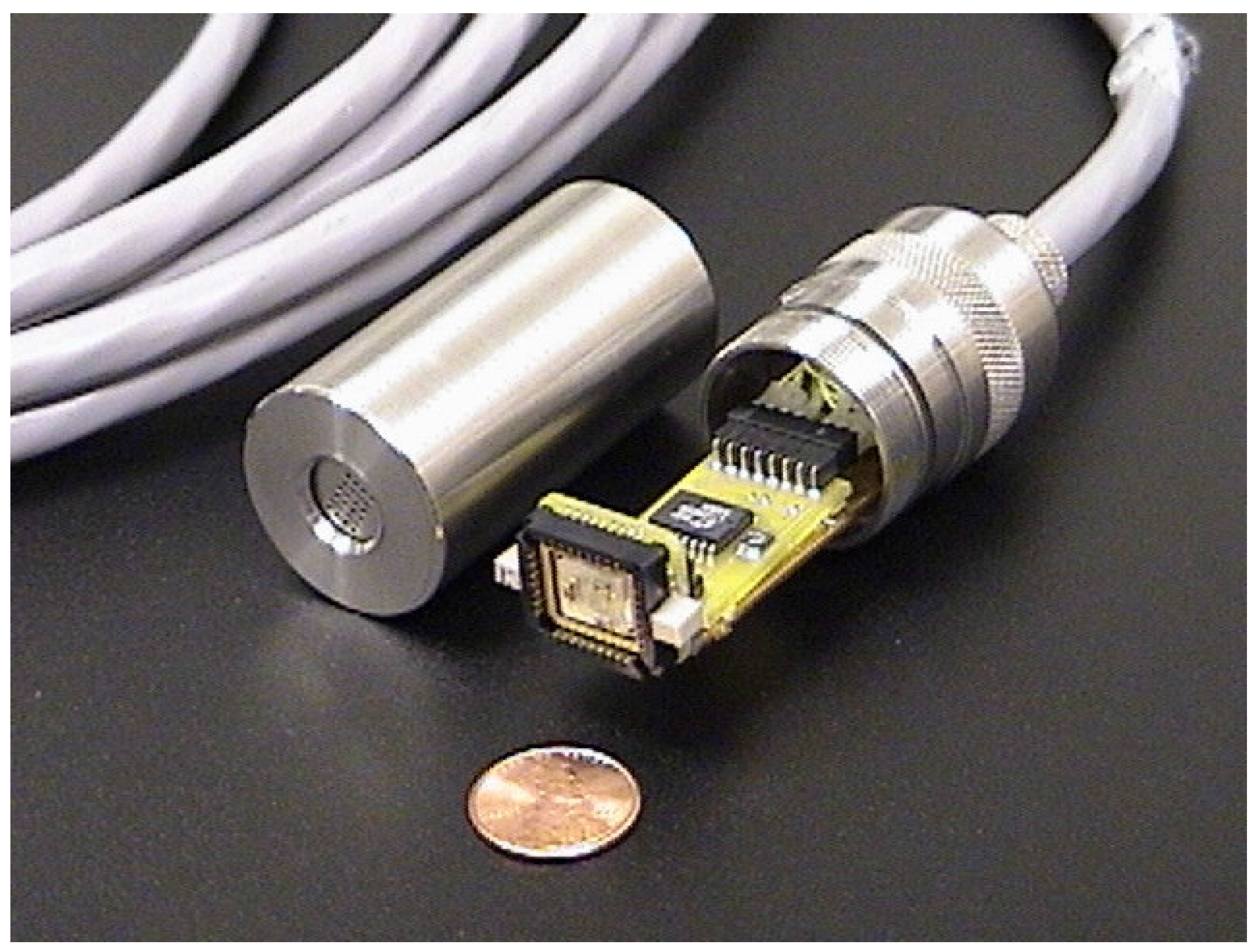
Figure 1.
Left: Four-channel SAW packaged in a leadless chip carrier. Right: Close-up of four channels for SAW P9. Three of the four have polymer depositions. The fourth channel (circled) is the reference channel. Black circles are polymer depositions (the circles outside the SAW transducers were practice depositions).
The assembly consists of a stainless steel housing, a signal-conditioning board, a SAW interface circuit board, a supporting structure for the circuits, a sensor cap, and a manifold for a future pre-concentrator (see
Figure 2). The signal-conditioning board contains a four-channel op-amp (three are used) and associated resistors (unity gain), a voltage regulator (see below), and interface connectors. The op-amp provides isolation, and therefore some level of protection, between the SAW and the measuring equipment. The SAW interface circuit board carries the traces to the SAW socket/LCC.
The voltage regulator was to provide the 3.3 Volts DC (VDC) required by the SAW. However, the required 3.3 VDC was not maintained with the SAW device drawing its nominal 100-110 mA. As a result, the voltage regulator was replaced with an external potted power supply. This alternative external power supply worked very well—the only required input was 12-30 VDC, and the device outputs both 3.3 VDC for the SAW power and +/- 15 VDC for the op-amp power.
A stainless steel frame provides structural support for the circuit board. An electrically isolating tape was applied to the stainless steel to prevent shorting the traces on the circuit boards. A stainless steel cap fits over the circuit board and frame and screws into the bottom part of the housing (like a flashlight). Viton O-rings are used to provide a water-tight seal at all mating surfaces.
A unique feature of this assembly is the use of a Gore-Tex
® membrane (not shown in
Figure 2) that covers a perforated section of the sensor cap. The membrane prevents liquid water from seeping into the housing, but it allows gas-phase constituents to pass into the headspace of the SAW sensor. If the assembly is immersed in water, aqueous-phase compounds can volatilize and partition across the membrane into the gas-phase headspace, where they can be detected by the SAW sensor.
Figure 2.
Integrated SAW probe for in-situ monitoring applications. The Gore-Tex® membrane that covers the perforated section of the cap is not shown.
Figure 2.
Integrated SAW probe for in-situ monitoring applications. The Gore-Tex® membrane that covers the perforated section of the cap is not shown.
Polymer Selection
The polymer selection for use with the SAW sensors was based on the work of Grate et al
. [
4] and Abraham et al. [
5], who characterized 14 polymers and developed a methodology for estimating the responses of polymer-coated SAW sensors to a wide range of vapor phase analytes. They describe how to use linear solvation energy relationships (LSERs) to model the sorption of vapors by polymer layers. The overall sorption process (where the vapor is the solute and the polymer is the solvent) is modeled as a linear combination of particular interactions (e.g. polarity, acidity basicity). These solvation parameters have been determined for many organic solutes and the values for common chlorinated solvents important to DOE are shown in
Table 1. Also shown in
Table 2 are the solvation parameters for water because this is a potentially significant interfering species for environmental monitoring applications.
Table 2 lists the LSER experimentally determined coefficients for 14 polymers and oligomers of which some are commercially available but most are not. A polymer/vapor partition coefficient is estimated by combining the coefficients for a given polymer with the solvation parameters of a given vapor species.
Table 3 lists the logarithm of the partition coefficients for the possible polymer/vapor combinations from
Table 1 and
Table 2.
Finally,
Table 4 lists an estimated detection limit for a hypothetical SAW device for each of the targeted chlorinated VOCs with each of the 14 coating. The equation used to calculate these estimated detection limits is Equation 7 in Grate et al. [
4], but a coefficient of 2 was used rather than the coefficient of 4 as shown in the paper (personnel communication with Jay Grate, 2002). This calculation assumes a 500 MHz SAW device coated with a mass of polymer that shifts the frequency of the device by 1500 kHz and a detection sensitivity of 50 Hz. (Note that the SAW array devices used in this study registers a phase shift that produces a change in output voltage. The output voltage is not easily compared to a typical frequency-shift device. Approximate parameters for rough comparison are a polymer mass resulting in a 1-volt signal change and a detection sensitivity of 0.04 mV)
The purpose of
Table 4 is to provide a rough relative comparison of the detection sensitivity of the 14 polymers for screening purposes. What is desired is a low estimated detection limit for a desired target VOC and a high detection limit for water, which generally acts as an interfering species. The polymer poly(vinyl tetradecanal) (PVTD) has the lowest (or next lowest) estimated detection limit for all of the VOCs of interest and a reasonably high detection limit for water. This polymer was also readily synthesized in-house at Sandia and was therefore chosen for use in this study. PVTD was used on two of the three SAW channels. Another polymer chosen was polyisobutylene (PIB), a commercially available polymer with reasonably low estimated detection limits for the targeted VOCs and the highest detection limit for water.
Table 1.
Solvation parameters for selected chlorinated VOCs and water (from [
5]).
Table 1.
Solvation parameters for selected chlorinated VOCs and water (from [5]).
| VOC → | PCE | TCE | t-1,2 DCE | c-1,2 DCE | 1,1 DCE | CCl4 | TCM | DCM | CM | Water |
|---|
| R2 | 0.639 | 0.524 | 0.425 | 0.436 | 0.362 | 0.458 | 0.425 | 0.387 | 0.249 | 0.000 |
| πH2 | 0.420 | 0.400 | 0.410 | 0.610 | 0.340 | 0.380 | 0.490 | 0.570 | 0.430 | 0.450 |
| ΣαH2 | 0.000 | 0.080 | 0.090 | 0.110 | 0.000 | 0.000 | 0.150 | 0.100 | 0.000 | 0.820 |
| ΣβH2 | 0.000 | 0.030 | 0.050 | 0.050 | 0.050 | 0.000 | 0.020 | 0.050 | 0.080 | 0.350 |
| Log L16 | 3.584 | 2.997 | 2.278 | 2.439 | 2.110 | 2.823 | 2.480 | 2.019 | 1.163 | 0.260 |
| Log LW | -0.070 | 0.320 | 0.570 | 0.860 | -0.180 | -0.060 | 0.790 | 0.960 | 0.400 | 4.640 |
| Vx | 0.837 | 0.715 | 0.592 | 0.592 | 0.592 | 0.739 | 0.617 | 0.494 | 0.372 | 1.028 |
Optimization
A report from the GE Research & Development Center [
6] describes their efforts to dramatically increase the sensitivity of an acoustic wave sensor. They found that optimal performance was achieved by optimizing both the gate time, over which the data was averaged, and the thickness of the polymer coating. Control over the gate time, or the number of sensor readings used in a running average, was easily achieved with our data logger and thus was the focus of our optimization efforts. Control of the polymer coating thickness is more difficult.
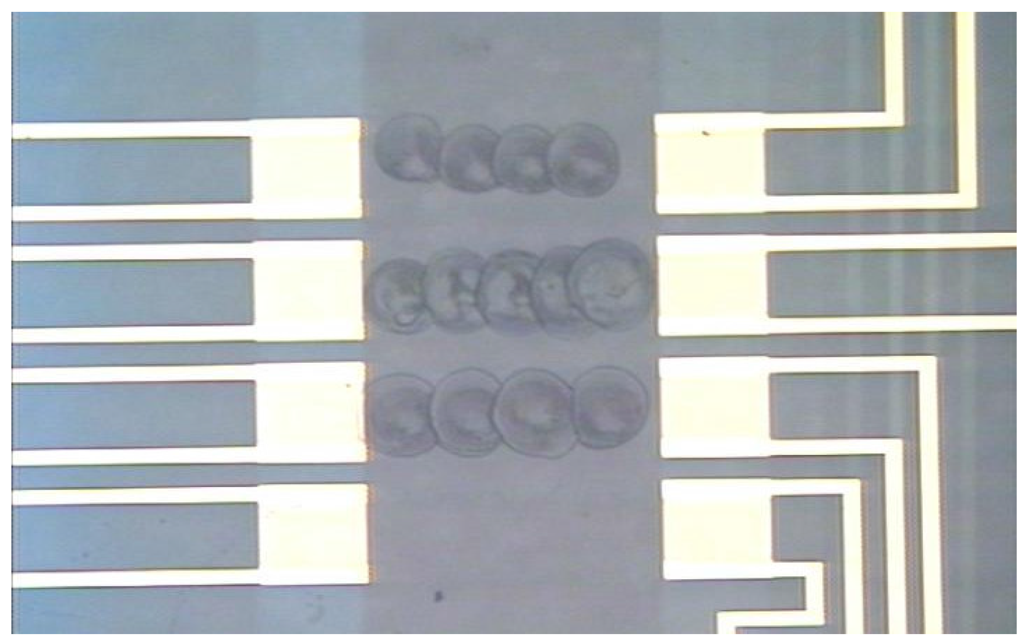
Utilizing the standard picospritzed technique, three SAW arrays were coated with PIB and PVTD. Only qualitative efforts were made to optimize the coatings, and the surface of the coatings were visibly rippled when viewed under a microscope as shown in
Figure 3. It is postulated that this rippled surface primarily results from the rapid evaporation of the solvent. Slowing the solvent evaporation may allow the polymer surface to flatten before it sets. A rippled surface necessarily means there is a variation in the coating thickness; thus, an optimal thickness is difficult to achieve.
Table 2.
Linear solvation energy relationship (LSER) coefficients for 14 polymers and oligomers (from [
4]).
Table 2.
Linear solvation energy relationship (LSER) coefficients for 14 polymers and oligomers (from [4]).
| C | r | s | a | b | l |
|---|
| PIB | -0.766 | -0.077 | 0.366 | 0.180 | 0.000 | 1.016 |
| PECH | -0.749 | 0.096 | 1.628 | 1.450 | 0.707 | 0.831 |
| OV25 | -0.846 | 0.177 | 1.287 | 0.556 | 0.440 | 0.885 |
| OV202 | -0.391 | -0.480 | 1.298 | 0.441 | 0.705 | 0.807 |
| PVPR | -0.571 | 0.674 | 0.828 | 2.246 | 1.026 | 0.718 |
| PVTD | -0.591 | -0.016 | 0.736 | 2.436 | 0.224 | 0.919 |
| PEM | -1.653 | -1.032 | 2.754 | 4.226 | 0.000 | 0.865 |
| SXCN | -1.630 | 0.000 | 2.283 | 3.032 | 0.516 | 0.773 |
| PEI | -1.580 | 0.495 | 1.516 | 7.018 | 0.000 | 0.770 |
| SXPYR | -1.938 | -0.189 | 2.425 | 6.780 | 0.000 | 1.016 |
| SXFA | -0.084 | -0.417 | 0.602 | 0.698 | 4.250 | 0.718 |
| FPOL | -1.207 | -0.672 | 1.446 | 1.494 | 4.086 | 0.810 |
| P4V | -1.329 | -1.538 | 2.493 | 1.507 | 5.877 | 0.904 |
| ZDOL | -0.486 | -0.750 | 0.606 | 1.441 | 3.668 | 0.709 |
Table 3.
log K =
c +
r R
2 +
sπ
H2+
aΣα
H2 +
bΣβ
H2 + /Log L
16 calculated from values in
Table 1 and
Table 2.
Table 3.
log K = c + r R2 + sπH2+ aΣαH2 + bΣβH2 + /Log L16 calculated from values in Table 1 and Table 2.
| PCE | TCE | t-1,2 DCE | c-1,2 DCE | 1,1 DCE | CCl4 | TCM | DCM | CM | Water |
|---|
| PIB | 2.9799 | 2.3994 | 1.6820 | 1.9215 | 1.4743 | 2.2060 | 1.9273 | 1.4821 | 0.5538 | -0.1895 |
| PECH | 2.9744 | 2.5802 | 2.0181 | 2.5076 | 1.6280 | 2.2595 | 2.3820 | 2.0743 | 0.9980 | 1.6361 |
| OV25 | 2.9795 | 2.4716 | 1.8450 | 2.2579 | 1.5450 | 2.2225 | 2.1469 | 1.8205 | 0.8159 | 0.5732 |
| OV202 | 2.7397 | 2.3517 | 1.8505 | 2.2435 | 1.6146 | 2.1606 | 2.1226 | 1.8718 | 1.0426 | 1.0113 |
| PVPR | 2.7808 | 2.4757 | 1.9440 | 2.2775 | 1.5208 | 2.0792 | 2.2592 | 1.8873 | 0.8700 | 2.1891 |
| PVTD | 3.0016 | 2.6509 | 2.0279 | 2.3716 | 1.6037 | 2.2757 | 2.4118 | 1.9326 | 0.8082 | 2.0551 |
| PEM | 1.9444 | 1.8383 | 1.3884 | 2.1516 | 0.7349 | 1.3628 | 2.0370 | 1.6864 | 0.2802 | 3.2765 |
| SXCN | 2.0993 | 1.8579 | 1.3656 | 2.0073 | 0.8031 | 1.4197 | 1.8708 | 1.5610 | 0.2920 | 2.2652 |
| PEI | 2.1327 | 2.1549 | 1.6376 | 2.2106 | 0.7393 | 1.3965 | 2.3355 | 1.7321 | 0.0906 | 5.0572 |
| SXPYR | 2.6011 | 2.5203 | 1.9006 | 2.6827 | 0.9618 | 1.7651 | 2.7066 | 2.1004 | 0.2393 | 4.9770 |
| SXFA | 2.4757 | 2.2735 | 1.8965 | 2.1419 | 1.6972 | 1.9807 | 2.0041 | 1.8297 | 1.2461 | 2.4334 |
| FPOL | 1.8740 | 1.6889 | 1.2842 | 1.7263 | 0.9548 | 1.3213 | 1.5306 | 1.3462 | 0.5164 | 2.3095 |
| P4V | 1.9752 | 1.8684 | 1.5283 | 2.1856 | 1.1632 | 1.4659 | 1.8244 | 1.7665 | 0.8815 | 3.3206 |
| ZDOL | 1.8303 | 1.7136 | 1.3719 | 1.6278 | 1.1279 | 1.4023 | 1.5400 | 1.3281 | 0.7058 | 2.4365 |
Table 4.
Polymer detection estimate in ppmv calculated using: C
v= Δf
v/(2Δf
sK/ρ
s )* (Adapted from [
4]).
Table 4.
Polymer detection estimate in ppmv calculated using: Cv= Δfv/(2ΔfsK/ρs )* (Adapted from [4]).
| VOC | | PCE | TCE | c-1,2 DCE | t-1,2 DCE | 1,1DCE | CCl4 | TCM | DCM | CM | Water |
|---|
| Mwt → | | 165.83 | 131.4 | 96.94 | 96.94 | 96.94 | 153.8 | 119.5 | 85.0 | 50.4 | 18.0 (g/mol) |
| Polymer | ρs (g/cm3) | | | | | | | | | | |
| PIB | 0.918 | 2.4 | 11.3 | 80.3 | 46.2 | 129.5 | 15.1 | 37.0 | 145.0 | 2073.5 | 32152.0 |
| PECH | 1.360 | 3.5 | 11.1 | 54.8 | 17.8 | 134.6 | 19.8 | 19.2 | 54.9 | 1104.7 | 711.6 |
| OV25 | 1.150 | 3.0 | 12.0 | 69.1 | 26.7 | 137.8 | 18.3 | 28.0 | 83.3 | 1420.5 | 6955.9 |
| OV202 | 1.252 | 5.6 | 17.3 | 74.3 | 30.0 | 127.8 | 22.9 | 32.2 | 80.6 | 917.7 | 2761.5 |
| PVPR | 1.010 | 4.1 | 10.5 | 48.3 | 22.4 | 128.0 | 22.3 | 19.0 | 62.8 | 1101.6 | 147.9 |
| PVTD | 0.960 | 2.4 | 6.7 | 37.8 | 17.2 | 100.5 | 13.5 | 12.7 | 53.7 | 1207.0 | 191.4 |
| PEM | 1.353 | 37.8 | 60.9 | 232.6 | 40.1 | 1047.0 | 155.5 | 42.4 | 133.5 | 5737.4 | 16.2 |
| SXCN | 1.120 | 21.9 | 48.2 | 202.9 | 46.3 | 740.9 | 112.9 | 51.4 | 147.5 | 4622.9 | 137.7 |
| PEI | 1.050 | 19.0 | 22.8 | 101.7 | 27.2 | 804.4 | 111.6 | 16.5 | 93.3 | 6889.9 | 0.2 |
| SXPYR | 1.000 | 6.2 | 9.4 | 52.8 | 8.7 | 458.9 | 45.5 | 6.7 | 38.0 | 4659.8 | 0.2 |
| SXFA | 1.477 | 12.1 | 24.4 | 78.8 | 44.8 | 124.7 | 40.9 | 49.9 | 104.8 | 677.6 | 123.2 |
| FPOL | 1.653 | 54.3 | 104.9 | 361.1 | 130.5 | 771.1 | 209.0 | 166.1 | 357.0 | 4069.8 | 183.5 |
| P4V | 1.440 | 37.5 | 60.5 | 179.3 | 39.5 | 415.7 | 130.5 | 73.6 | 118.2 | 1529.3 | 15.6 |
| ZDOL | 1.800 | 65.4 | 107.9 | 321.3 | 178.3 | 563.6 | 188.9 | 177.0 | 405.3 | 2864.9 | 149.2 |
Figure 3.
Polymer coating on SAWs sensor as applied by the standard picospritzer technique. Note the ripples on the resulting surface.
Figure 3.
Polymer coating on SAWs sensor as applied by the standard picospritzer technique. Note the ripples on the resulting surface.
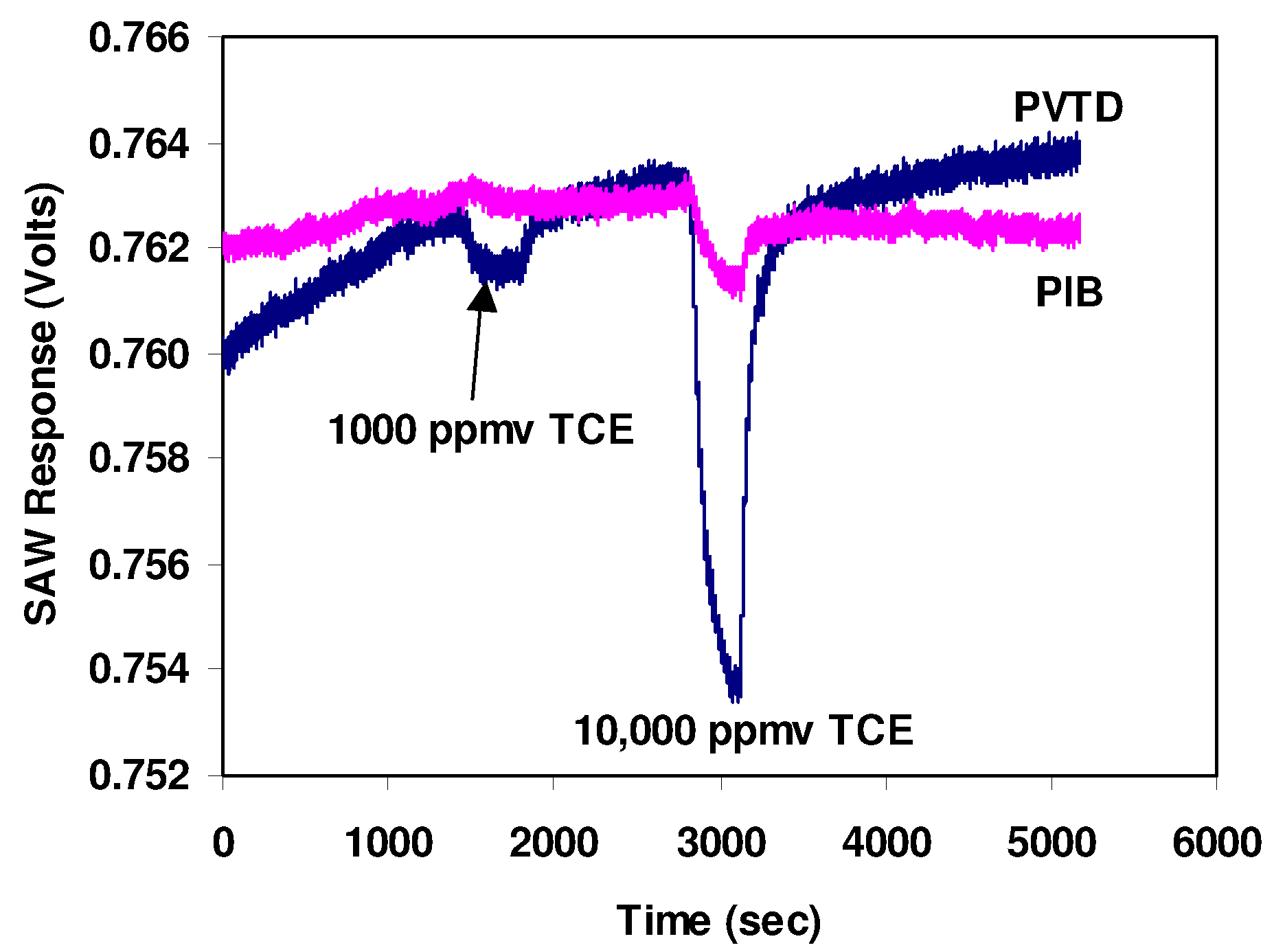
Figure 4 shows the output of one sensor when exposed to 1000 ppmv and 10,000 ppmv of trichloroethylene (TCE) calibration gases. These data were collected at a rate of 5 samples per second, the maximum rate achievable with our data-acquisition system. The standard deviation of the noise is about 0.13 mV which is within the expected range of 0.05 to 0.15 mV. As speculated, the PVTD coated sensor was more sensitive to TCE than the PIB coated sensor. However, the response or sensitivity to TCE was much lower than expected. The PVTD coating resulted in only a 1 mV signal when exposed to a 1000 ppmv TCE calibration gas and only about a 10 mV signal when exposed to a 10,000 ppmv TCE calibration gas.
Figure 4.
Output of SAWs sensor when exposed to 1,000 and 10,000 ppm TCE. Data were acquired at a rate of 5 samples per second.
Figure 4.
Output of SAWs sensor when exposed to 1,000 and 10,000 ppm TCE. Data were acquired at a rate of 5 samples per second.
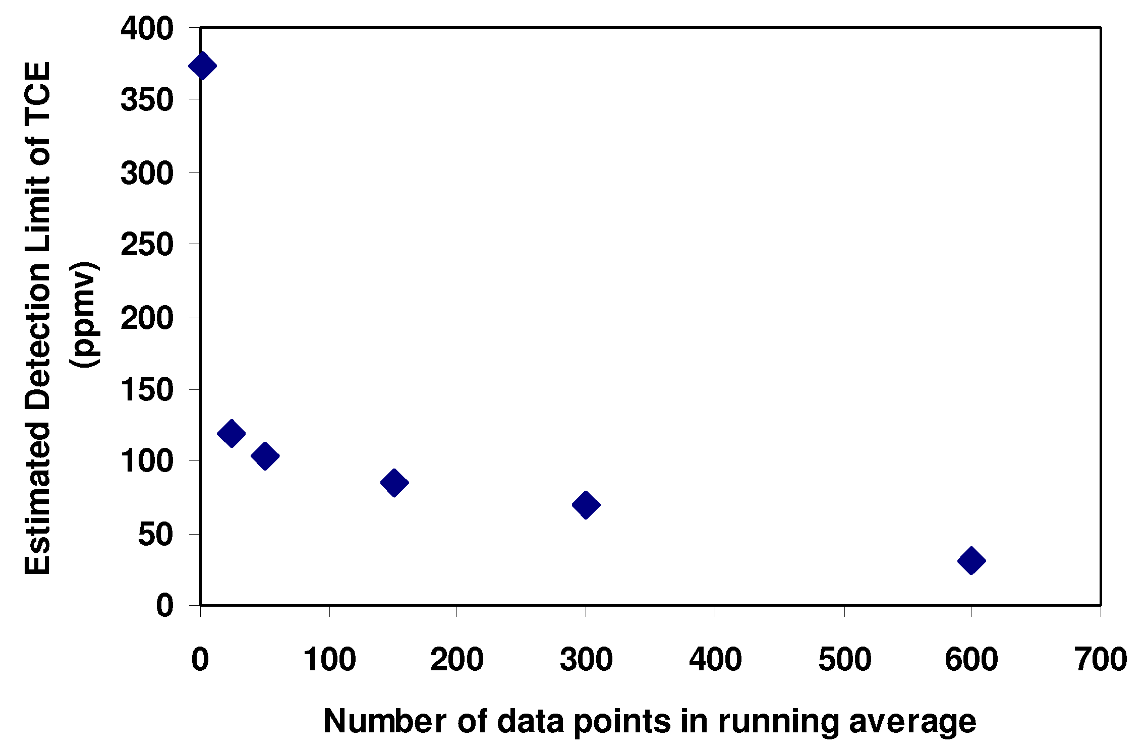
Figure 5 shows the same data processed as a running average using a time window or gate of 120 seconds (600 data points). As the gate time was increased, the standard deviation of the sensor noise decreased. The detection limit can be estimated by extrapolating the 1000 ppmv TCE response linearly to zero and defining the detection limit at three standard deviations above the noise.
Figure 6 shows the estimated detection limit as a function of the number of data points used in the running average. The detection limit was improved by just over an order of magnitude, which is similar to the improvement demonstrated in [
6].
Figure 5.
Data of
Figure 4 processed as a 120-second running average.
Figure 5.
Data of
Figure 4 processed as a 120-second running average.
Figure 6.
Estimated detection limit of SAW sensor for TCE as a function of the size of the running average.
Figure 6.
Estimated detection limit of SAW sensor for TCE as a function of the size of the running average.
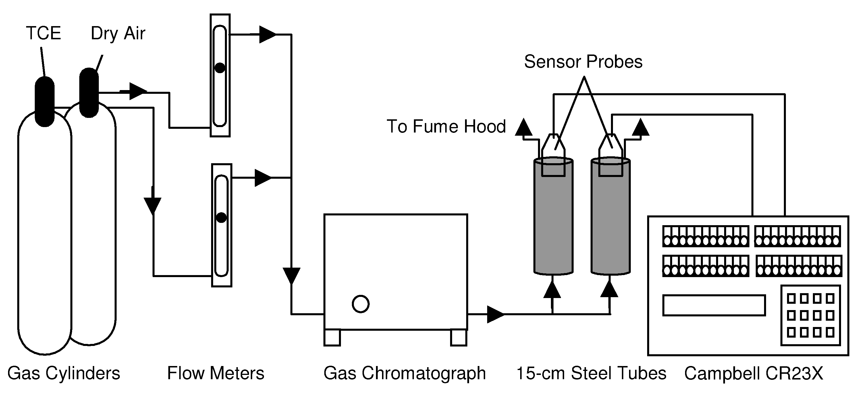
Calibration
The SAW sensors employing PVTD (two channels) and PIB (one channel) were calibrated using controlled concentrations of TCE. The sensors were placed in customized 15-cm steel tubes that allowed the sensors to be exposed to a flowing stream of varying concentrations of TCE vapor.
Figure 7 shows a schematic of the apparatus used for the calibrations.
Figure 7.
Schematic of apparatus for calibration experiment.
Figure 7.
Schematic of apparatus for calibration experiment.
The sensors were connected to a Campbell CR23X, which was programmed to read SAW output in DC volts. The SAW device required 3.3 V of input, so it was powered for approximately 2 hours prior to the beginning of the calibration run to ensure ample warm-up time. Dry air was passed across each sensor in order to remove the water vapor, and the sensors were allowed to reach equilibrium in the dry conditions. When the measured voltages were stable, the baseline was recorded and the calibration commenced. TCE vapor concentrations of 500, 1000, 5000, and 10,000 ppmv (parts per million by volume) were exposed to the sensors using customized gas cylinders containing 1,000 and 10,000 ppmv of TCE (500 and 5,000 ppmv were achieved through dilution with dry air from a compressed gas cylinder). TCE concentrations was measured using an MTI M200
™ micro-gas chromatograph. Following each exposure, dry air was used to purge the sensor and allow a new baseline to be established for the next exposure. The relative changes in voltage of the SAW sensors were used in the calibrations. The relative change is calculated as the maximum change in voltage divided by the baseline voltage for each exposure. The baseline value is calculated as a two-minute average prior to exposure to TCE. The maximum change is calculated by taking the difference between the baseline value and a value averaged for two minutes prior to shutting the TCE off. The TCE was turned off after the sensors had stabilized, which typically took 15-20 minutes. The relative changes in sensor signals (ΔV/V
b) were then plotted against the TCE concentration for each exposure using Microsoft Excel, and regressions were fit to the data.
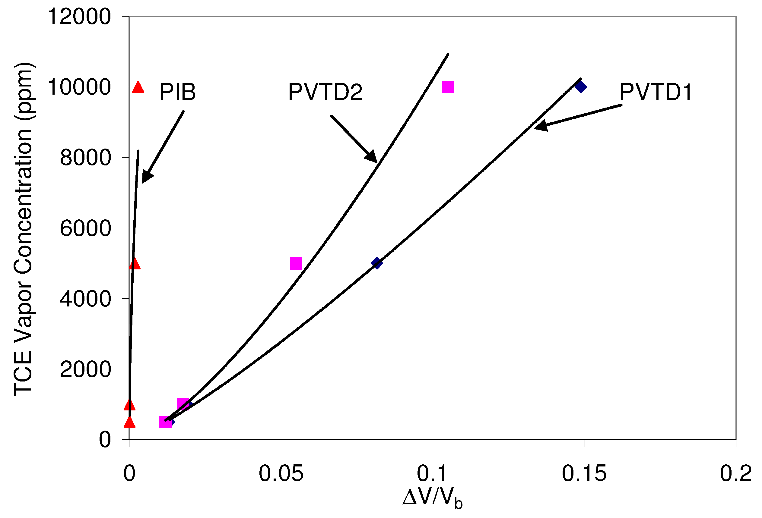
Figure 8 shows the results of the calibration run for SAW P9.
Figure 8.
Graph of the calibration of the SAW P9 to TCE under dry conditions.
Figure 8.
Graph of the calibration of the SAW P9 to TCE under dry conditions.
The polymer PVTD appeared responsive in the calibration runs. However, the polymer PIB on the SAW did not elicit a strong response to TCE. The responses of the polymers were fitted with a power function, and
Table 5 shows the regressions for the polymers on SAW P9 using two different units of concentration.
Field Test
The SAW sensor was evaluated side-by-side with a chemiresistor sensor in a simulated geologic environment at the Nevada Test Site. The sensors were placed in an outdoor “sandbox,” which consisted of a 1.2 m x 1.2 m x 0.6 m steel container that was filled with dry 20-40 mesh sand. Several PVC tubes (5 cm inner diameter) were placed vertically in the sand for sensor and contaminant emplacement. The chemiresistor and SAW sensors were placed in a vertical tube 25 cm away from the center. Additional sensors were placed in the tube to record barometric pressure, temperature, and
Table 5.
TCE calibrations for SAW P9 at room temperature (23 °C) in dry conditions.
Table 5.
TCE calibrations for SAW P9 at room temperature (23 °C) in dry conditions.
| Polymer | Regression Type | Concentration Regression (ppmv) | R2 | Concentration Regression (g/L) | R2 |
| PVTD1 | Power | y1 = 1.00E+05x1.20E+00 | 0.995 | y2 = 4.53E-01x1.20E+00 | 0.995 |
| PVTD2 | Power | y1 = 2.44E+05x1.38E+00 | 0.995 | y2 = 1.10E+00x1.38E+00 | 0.995 |
| PIB | Power | y1 = 2.02E+05x5.48E-01 | 0.936 | y2 = 9.13E-01x5.48E-01 | 0.936 |
humidity. In the experiments, trichloroethylene (TCE) was absorbed into a wick and then placed in the central tube. The sandbox was then insulated and data were recorded using a Campbell Scientific CR- 23X datalogger as the TCE vapors diffused through the sand to the sensors. The datalogger was programmed to perform a running average of the SAW-sensor response. Due to the complexity of the data-acquisition program (for collecting the SAW data, chemiresistor data, and environmental parameters) the SAW sensor response could only be read every 0.4 seconds and the averaging window was limited to 100 samples. Additional details of the experimental design and approach can be found in Ho et al. [
7].
Results showed that both the chemiresistor and SAW sensors were able to detect the emplacement and subsequent diffusion of TCE. However, the sensor responses were impacted by diurnal fluctuations in temperature and water-vapor concentrations. The SAW sensor, in particular, was strongly impacted by the variations in ambient temperature (16.8°C to 30.5°C) over a 48-day period.
Recommendations from this test included the use of statistical software packages such as Statistica
® to account for fluctuating environmental variables and multiple input channels (sensor array response) in multivariate predictions of chemical concentration. Efforts are currently ongoing to implement these multivariate models with the in-situ sensors. The use of preconcentrators [
7,
8] and automated temperature control [
7] were also recommended to improve the sensitivity and response of the sensors. It should be noted, however, that in actual subsurface applications, the temperature and water-vapor concentration should be quite stable.
Conclusions
A SAW sensor has been designed and developed to monitor volatile organic contaminants in subsurface environments. Unique features of this sensor include passive operation (no carrier gas) and waterproof packaging with a permeable membrane that allows it to be used in a variety of media. Calibrations of the sensor to a common groundwater contaminant (TCE) were performed in the laboratory, and studies were performed to optimize the performance of the sensor through polymer selection and signal averaging.
The performance of the SAW sensor was tested in the field [
7], and results showed that the response was impacted by diurnal and seasonal temperature/humidity fluctuations. Although univariate temperature corrections appeared to aid in the stability of the results, in-situ calibration (or re- baselining) is desirable to alleviate the impacts of drift or fluctuations in ambient conditions. Multivariate regression methods (e.g., using Statistica
®) that account for drift and multiple inputs and interferences (temperature, water-vapor pressure, etc.) are currently being investigated.
Acknowledgments
The authors thank Joy Byrnes, Steve Showalter, and Doug Adkins for their assistance with obtaining and coating the SAW devices. Sandia is a multiprogram laboratory operated by Sandia Corporation, a Lockheed Martin Company, for the United States Department of Energy under Contract DE-AC04-94AL85000.
References
- Frye, G.C. In situ field screening of volatile organic compounds using a portable acoustic wave sensor system, in Vadose Zone Science and Technology Solutions. Looney, B.B., Falta, R.W., Eds.; Battelle Press: Columbus, 2000; pp. 580–589. [Google Scholar]
- Ho, C.K.; Hughes, R.C. In-Situ Chemiresistor Sensor Package for Real-Time Detection of Volatile Organic Compounds in Soil and Groundwater. Sensors 2002, 2, 23–34. [Google Scholar] [CrossRef]
- Martin, S.J.; Frye, G.C.; Senturia, S.D. Dynamics and response of polymer-coated surface-acoustic-wave devices–effect of viscoelastic properties and film resonance. Analytical Chemistry 1994, 66(14), 2201–2219. [Google Scholar] [CrossRef]
- Grate, J.W.; Patrash, S.J.; Abraham, M.H. Method for estimating polymer-coated acoustic wave vapor sensor responses. Analytical Chemistry 1995, 67(13), 2162–2169. [Google Scholar] [CrossRef]
- Abraham, M.H.; Andonian-Haftvan, J.; Whiting, G.; Leo, A.; Taft, R.W. Hydrogen-Bonding .34. The Factors that Influence the Solubility Of Gases And Vapors In Water At 298-K, and a New Method For Its Determination. J. Chem. Soc., Perkins Trans. 1994, 2, 1777–1791. [Google Scholar] [CrossRef]
- Potyrailo, R.A.; Sivavec, T.M.; Bracco, A.A. 2001, Field Evaluation of Acoustic Wave Chemical Sensors for Monitoring of Solvents in Groundwater. GE Research & Development Center Report 2000CRD092. April 2001. [Google Scholar]
- Ho, C.K.; Wright, J.; McGrath, L.K.; Lindgren, E.R.; Rawlinson, K.S.; Lohrstorfer, C.F. 2003, Field Demonstrations of Chemiresistor and Surface Acoustic Wave Microchemical Sensors at the Nevada Test Site. SAND2003-0799, Sandia National Laboratories Report. Albuquerque, NM.
- Hughes, R. C.; Patel, S.V.; Manginell, R.P. 2000, A MEMS based hybrid preconcentrator/chemiresistor chemical sensor. In Proceedings of the 198th Meeting of the Electrochemical Society, Phoenix, AZ, 22 - 27 October 2000. SAND2000-1471C.
© 2003 by MDPI (http://www.mdpi.net). Reproduction is permitted for noncommercial purposes.


