Author Contributions
Conceptualization, Y.X. and J.X.; methodology, Y.X. and K.-M.L.; software, Y.X. and Y.W.; validation, Y.X. and Y.W.; formal analysis, W.W.; data curation, A.W.; writing—original draft preparation, Y.X.; writing—review and editing, J.X.; supervision, J.X.; funding acquisition, Y.X. All authors have read and agreed to the published version of the manuscript.
Figure 1.
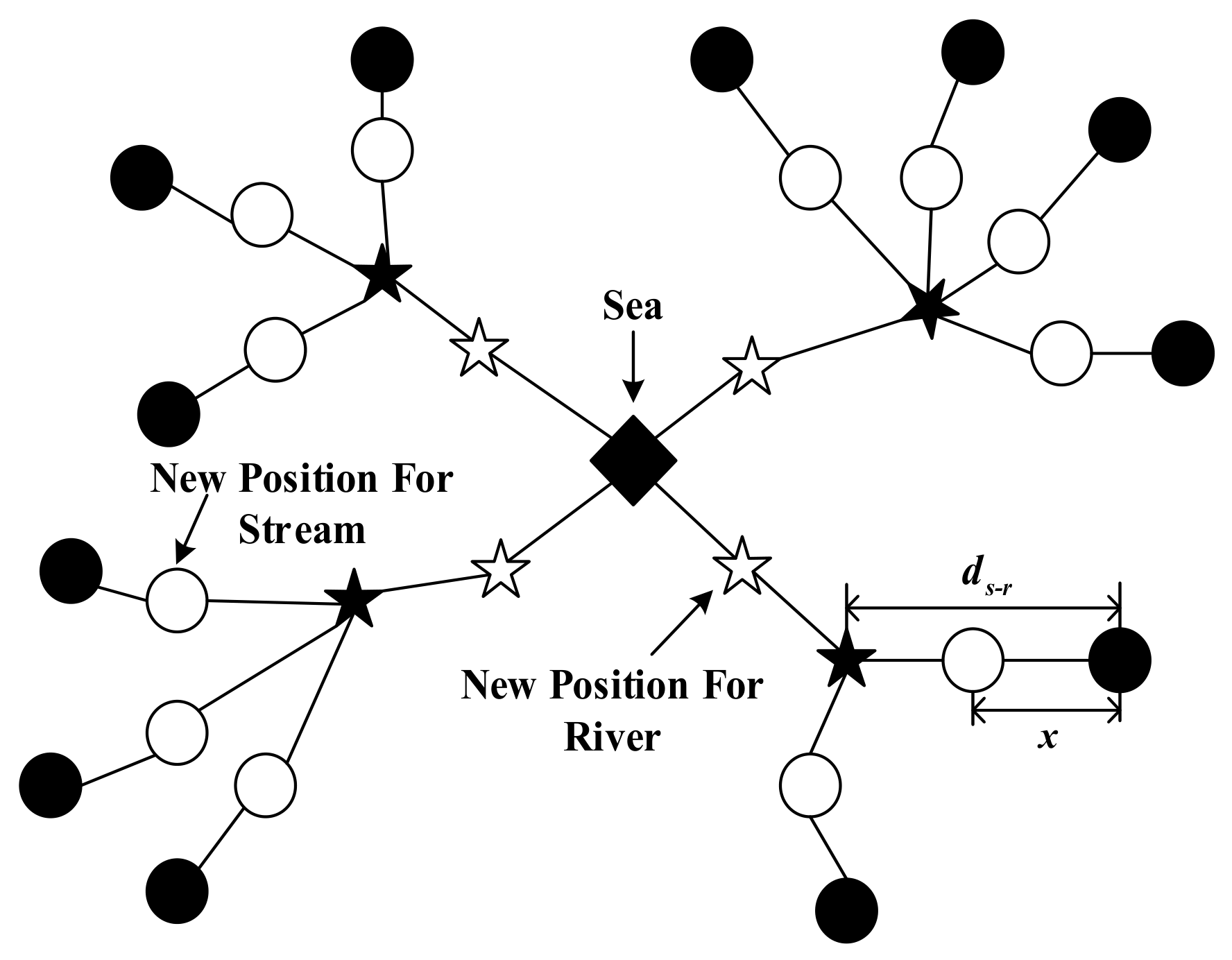
Brief schematic view of WCA [
33], where circles, stars, and the diamond correspond to the streams, rivers, and sea, respectively.
Figure 1.
Brief schematic view of WCA [
33], where circles, stars, and the diamond correspond to the streams, rivers, and sea, respectively.
Figure 2.
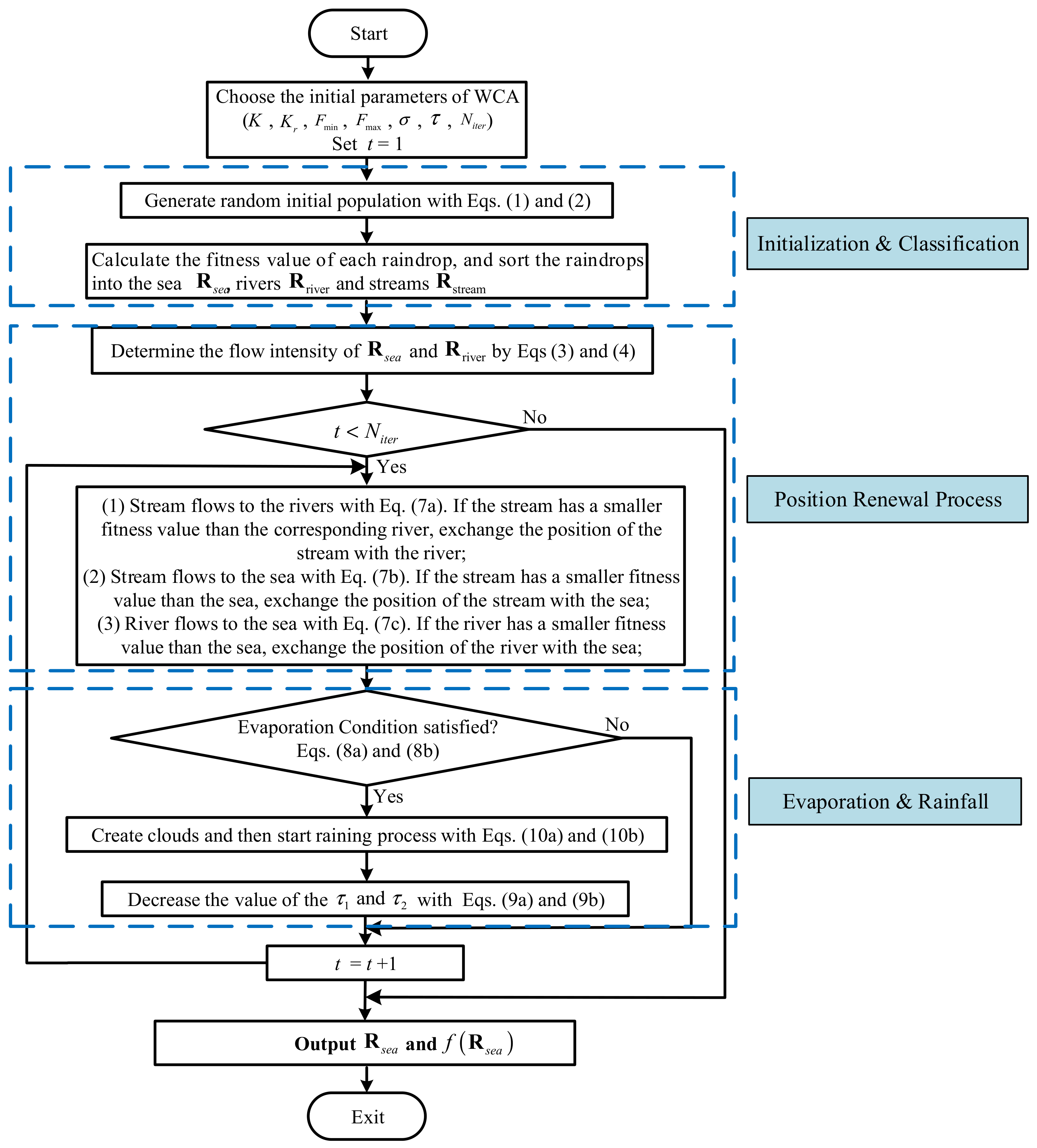
Flowchart of WCA.
Figure 2.
Flowchart of WCA.
Figure 3.
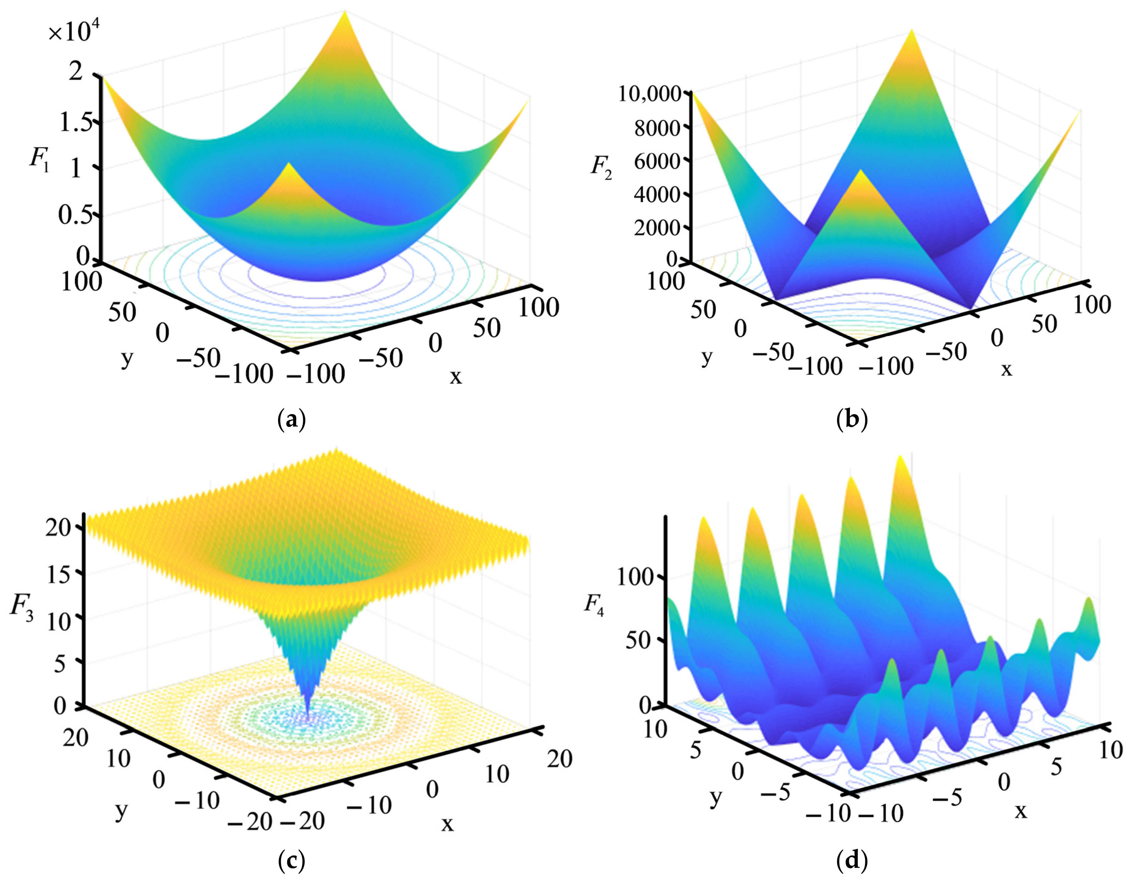
Illustration of the 2-D versions of (a) F1, (b) F2, (c) F3 and (d) F4.
Figure 3.
Illustration of the 2-D versions of (a) F1, (b) F2, (c) F3 and (d) F4.
Figure 4.
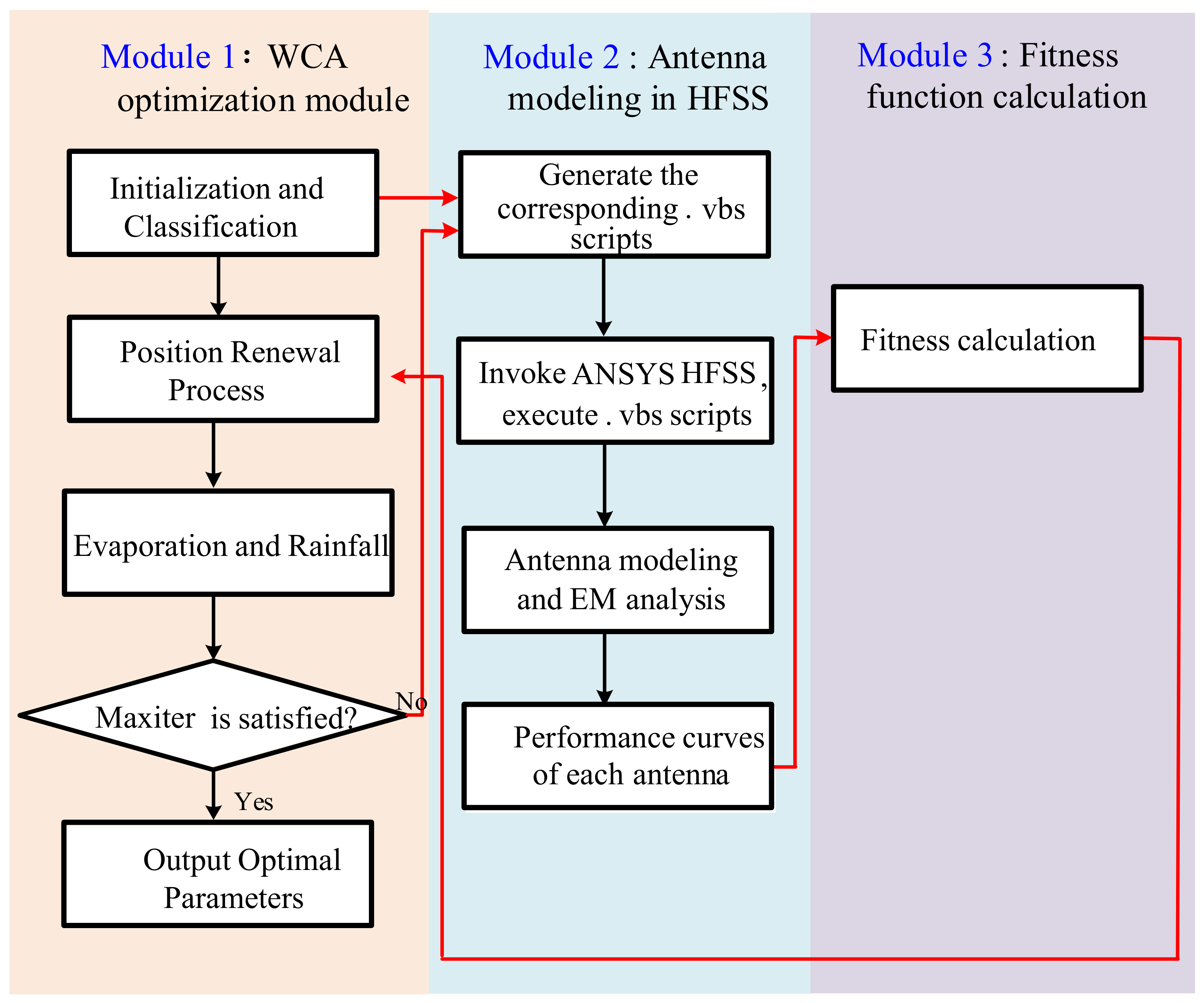
Flowchart of the WCA-based antenna optimization scheme.
Figure 4.
Flowchart of the WCA-based antenna optimization scheme.
Figure 5.
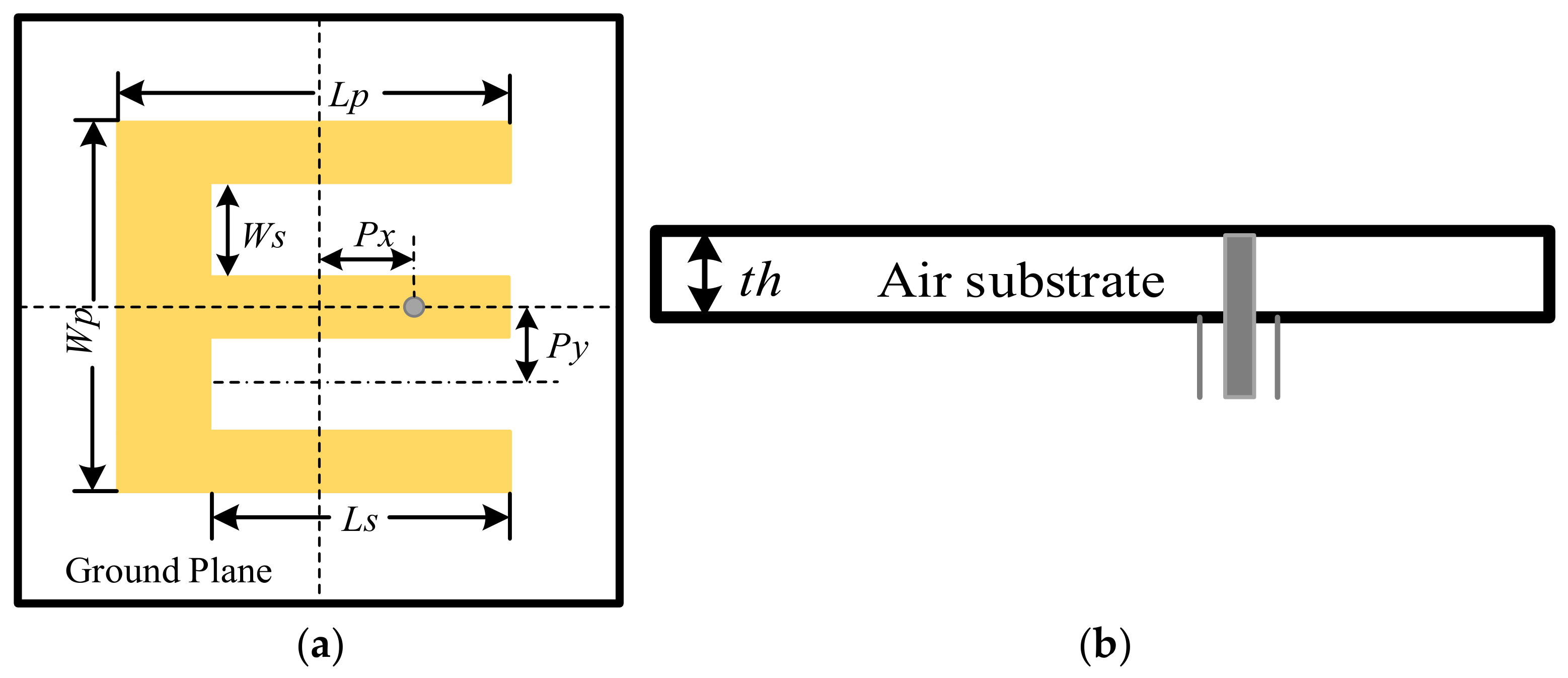
Geometry of E-shaped patch antenna. (a) Top view and (b) side view.
Figure 5.
Geometry of E-shaped patch antenna. (a) Top view and (b) side view.
Figure 6.
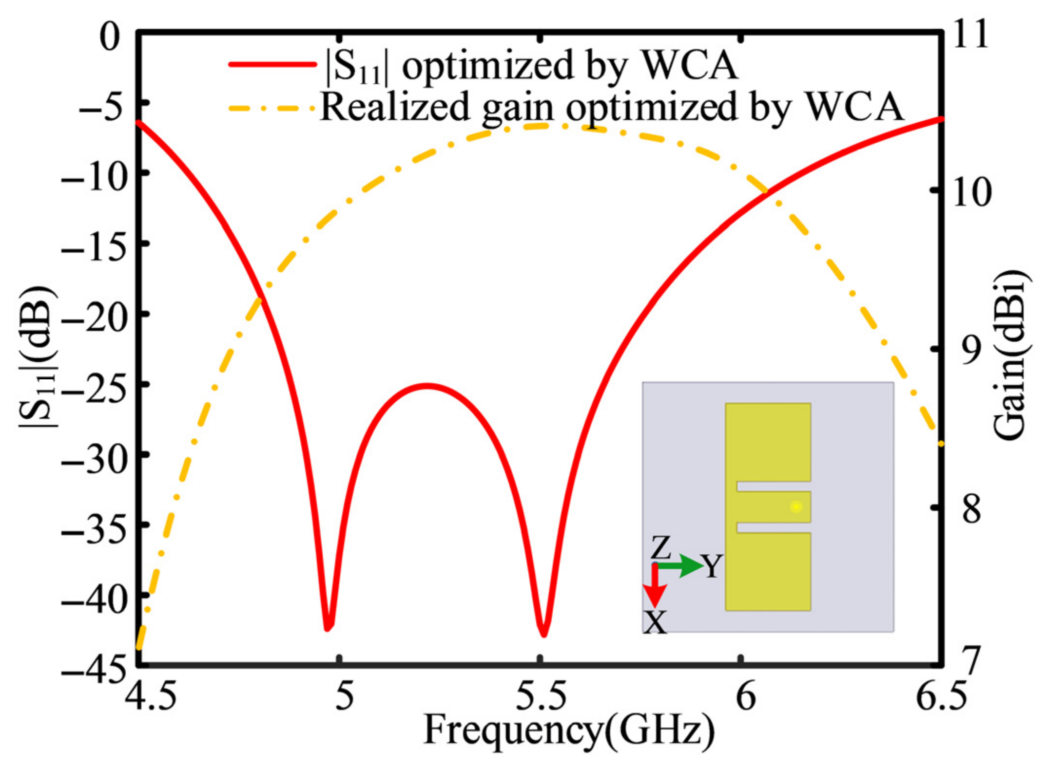
Simulated |S11| and realized gain curves of the optimized E-shaped patch antenna.
Figure 6.
Simulated |S11| and realized gain curves of the optimized E-shaped patch antenna.
Figure 7.
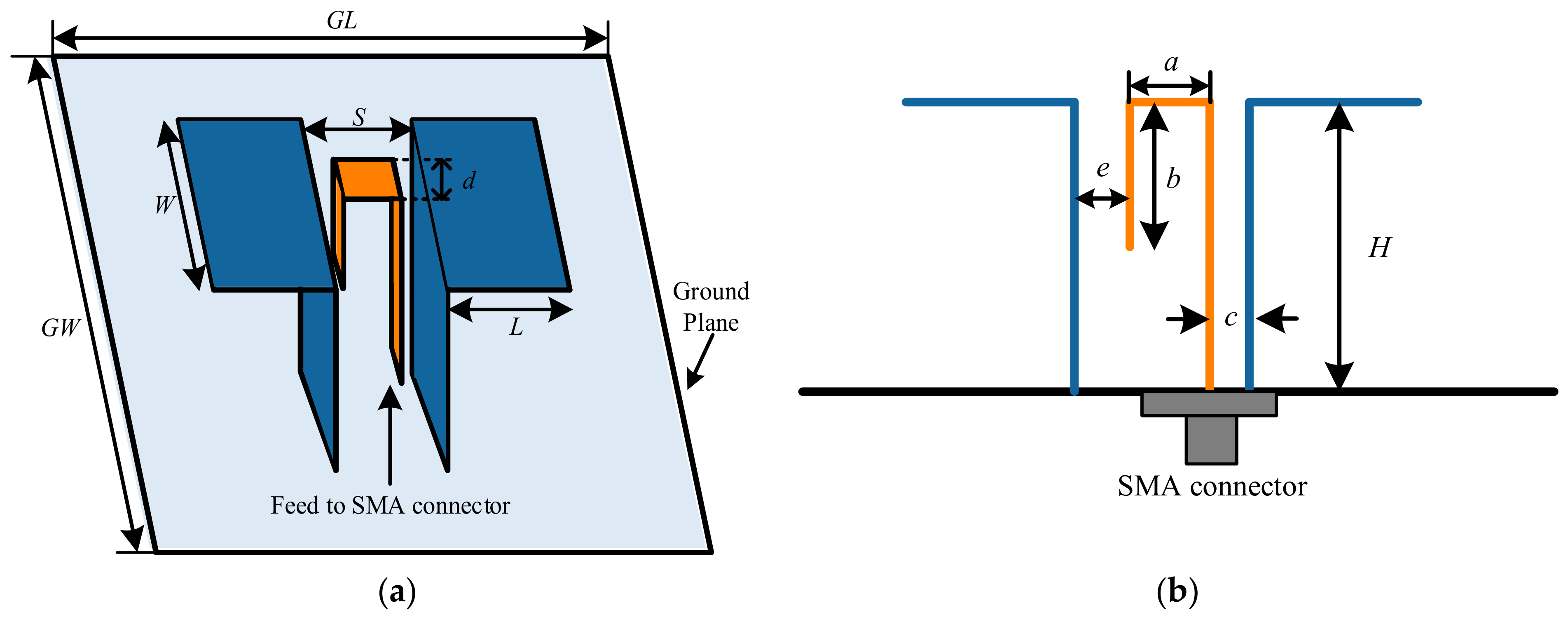
Geometry of conventional ME dipole antenna [
38]; (
a) 3D view and (
b) side view.
Figure 7.
Geometry of conventional ME dipole antenna [
38]; (
a) 3D view and (
b) side view.
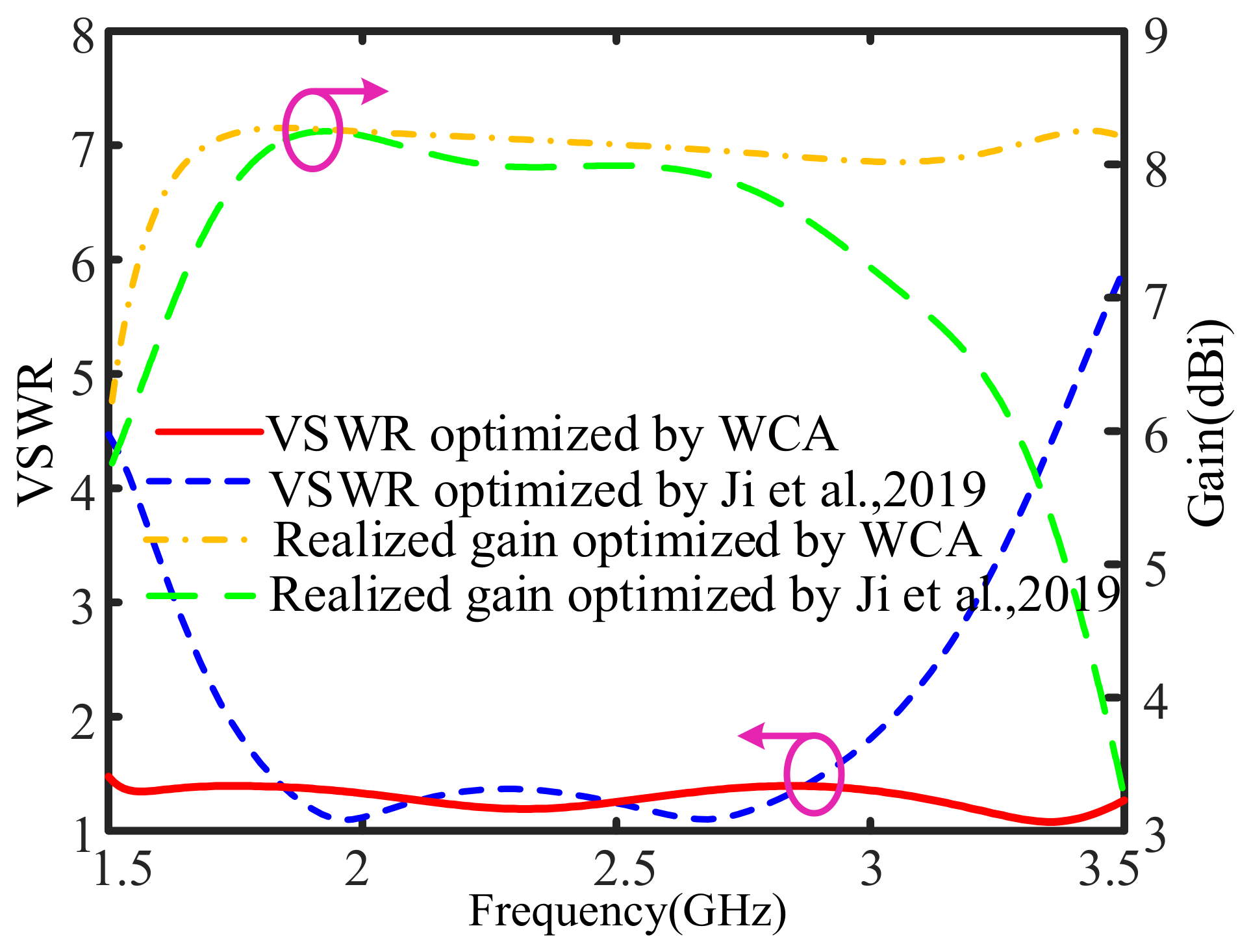
Figure 8.
Simulated VSWR and realized gain curve of the optimized ME dipole antenna [
35].
Figure 8.
Simulated VSWR and realized gain curve of the optimized ME dipole antenna [
35].
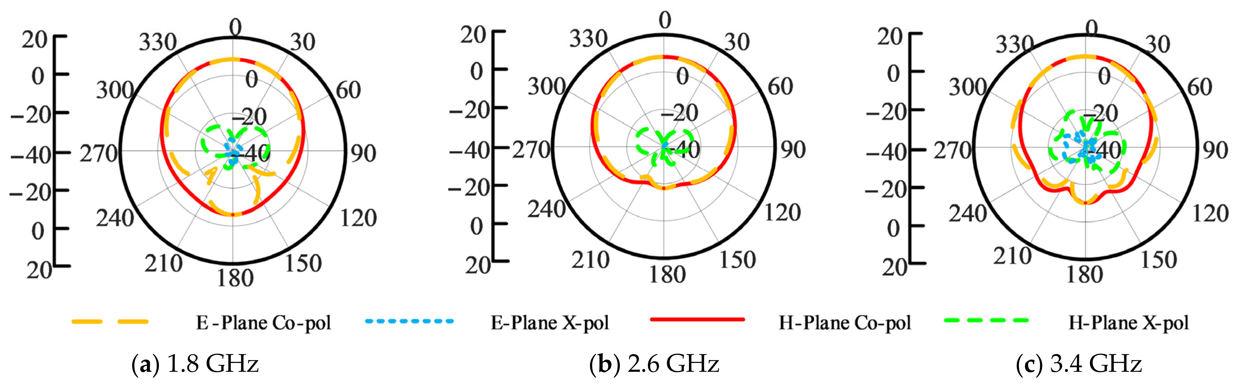
Figure 9.
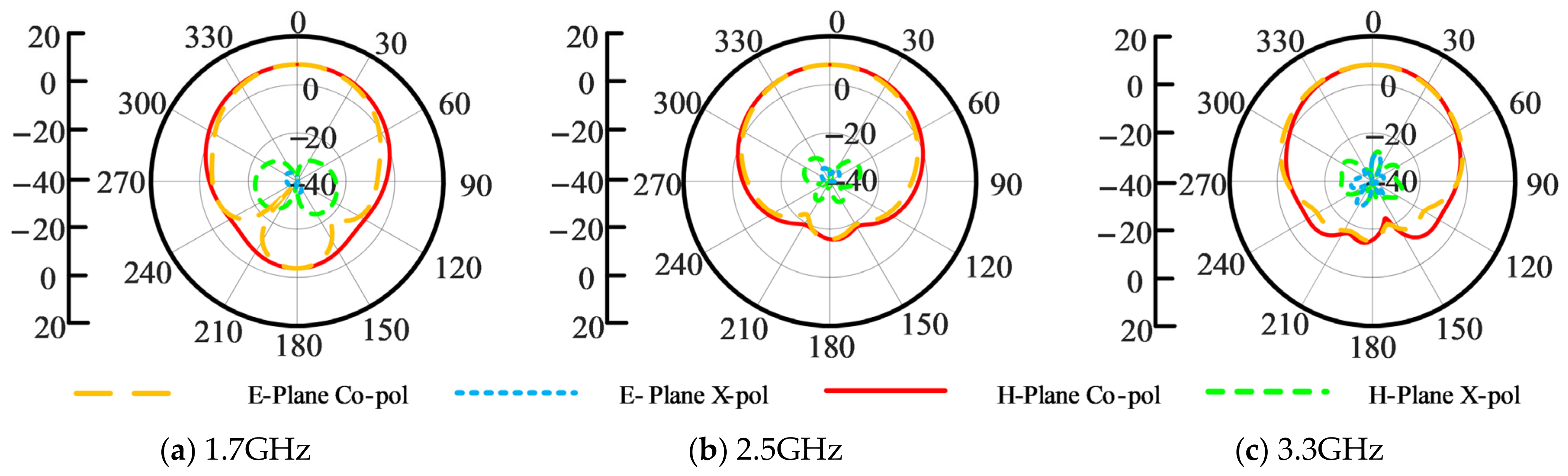
Simulated radiation patterns in E- and H-planes of the optimized ME dipole antenna at different frequencies; (a) 1.7 GHz, (b) 2.5 GHz and (c) 3.3 GHz.
Figure 9.
Simulated radiation patterns in E- and H-planes of the optimized ME dipole antenna at different frequencies; (a) 1.7 GHz, (b) 2.5 GHz and (c) 3.3 GHz.
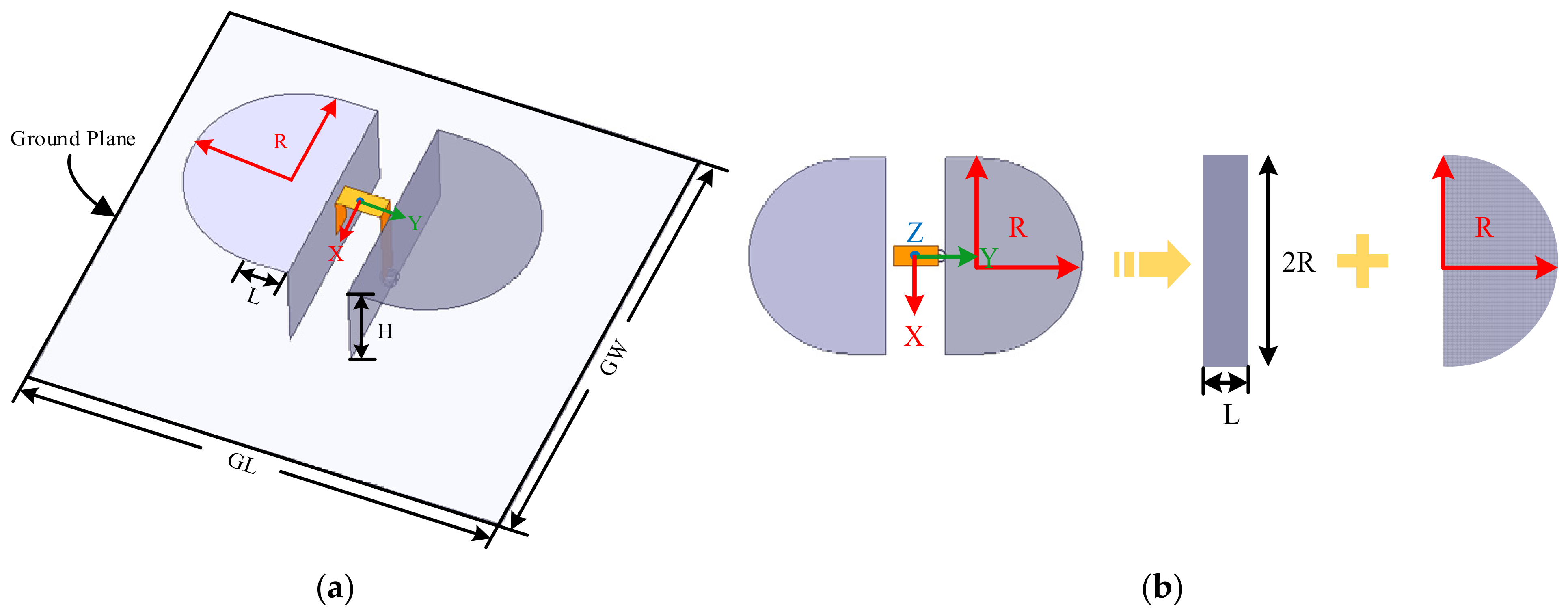
Figure 10.
Geometry of proposed ME dipole antenna; (a) 3D view and (b) top view.
Figure 10.
Geometry of proposed ME dipole antenna; (a) 3D view and (b) top view.
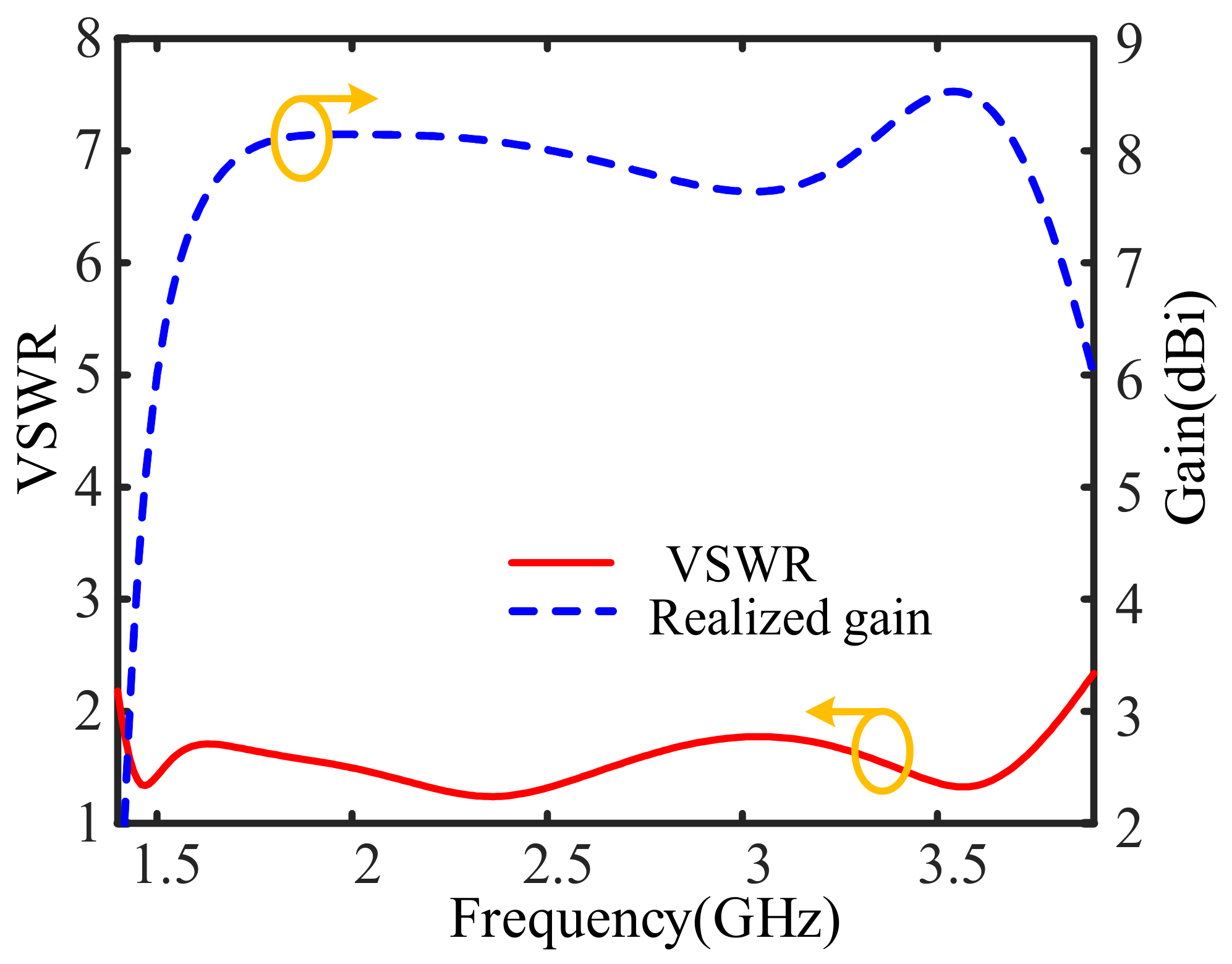
Figure 11.
Simulated VSWR and realized gain curves of the bandwidth-enhanced ME dipole antenna.
Figure 11.
Simulated VSWR and realized gain curves of the bandwidth-enhanced ME dipole antenna.
Figure 12.
Simulated radiation patterns of the optimized ME dipole antenna with enhanced bandwidth at different frequencies.
Figure 12.
Simulated radiation patterns of the optimized ME dipole antenna with enhanced bandwidth at different frequencies.
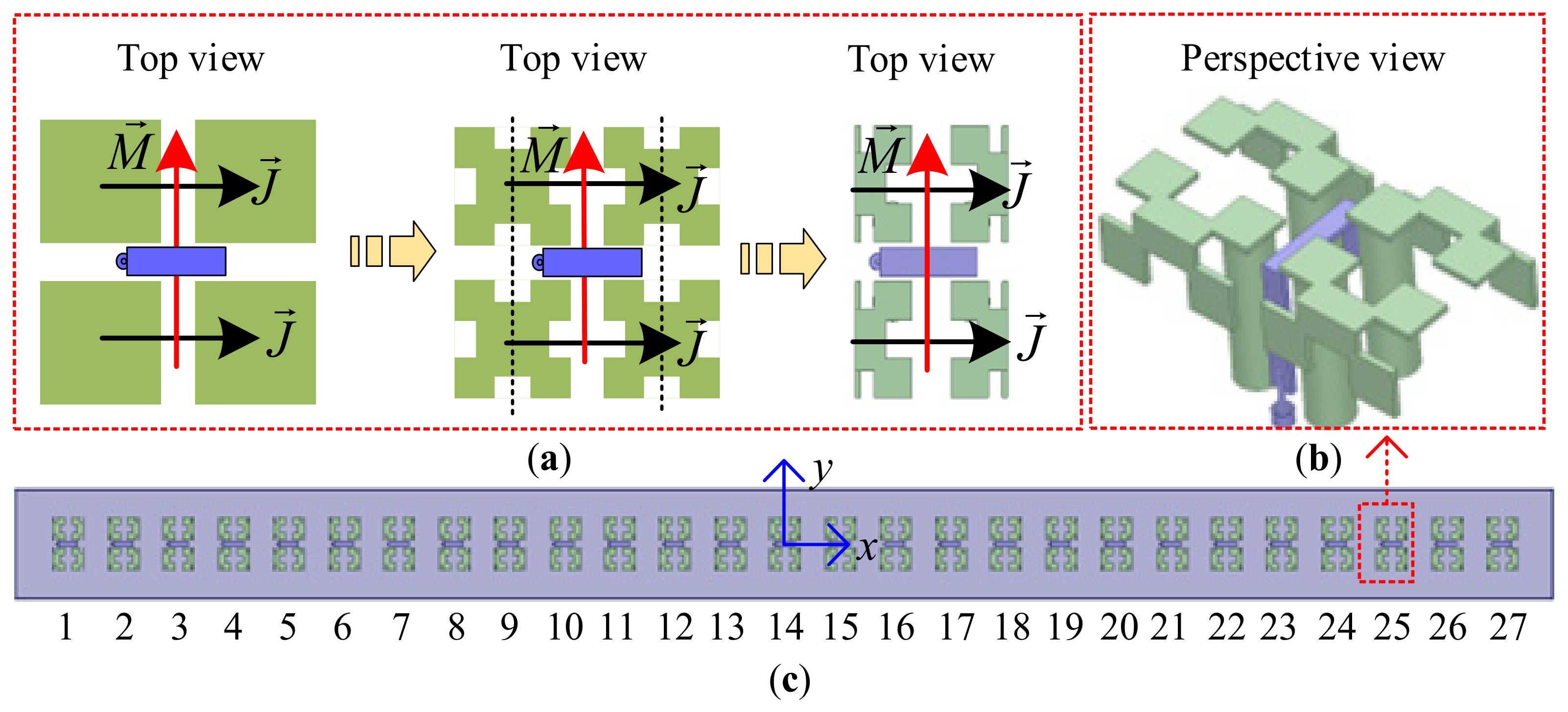
Figure 13.
Configuration of a uniformly spaced 27-element folded fractal ME dipole array antenna. (a) Design procedures of fractal ME dipole antenna, (b) perspective view of designed fractal ME dipole antenna and (c) uniformly spaced 27-element array antenna.
Figure 13.
Configuration of a uniformly spaced 27-element folded fractal ME dipole array antenna. (a) Design procedures of fractal ME dipole antenna, (b) perspective view of designed fractal ME dipole antenna and (c) uniformly spaced 27-element array antenna.
Figure 14.
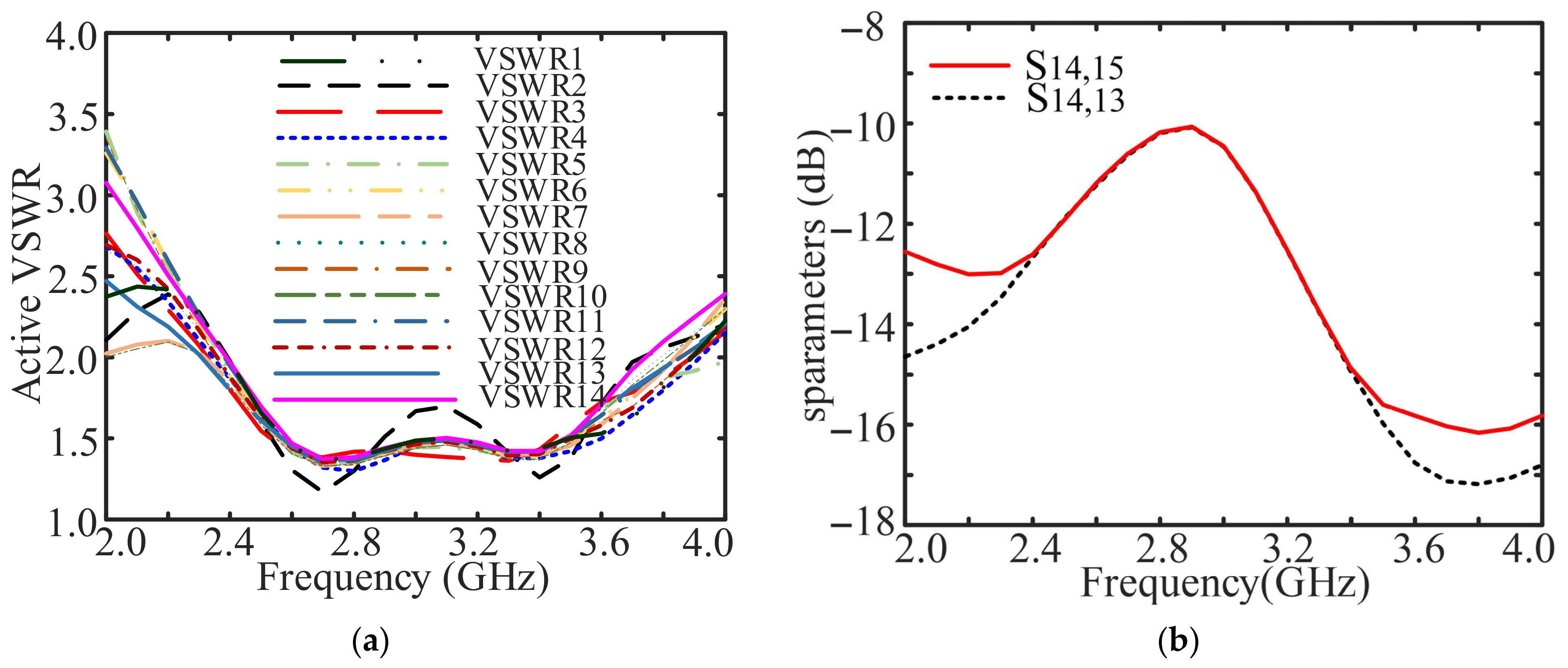
Simulated parameters of 27-element folded fractal ME dipole array antenna. (a) Active VSWRs and (b) S parameters.
Figure 14.
Simulated parameters of 27-element folded fractal ME dipole array antenna. (a) Active VSWRs and (b) S parameters.
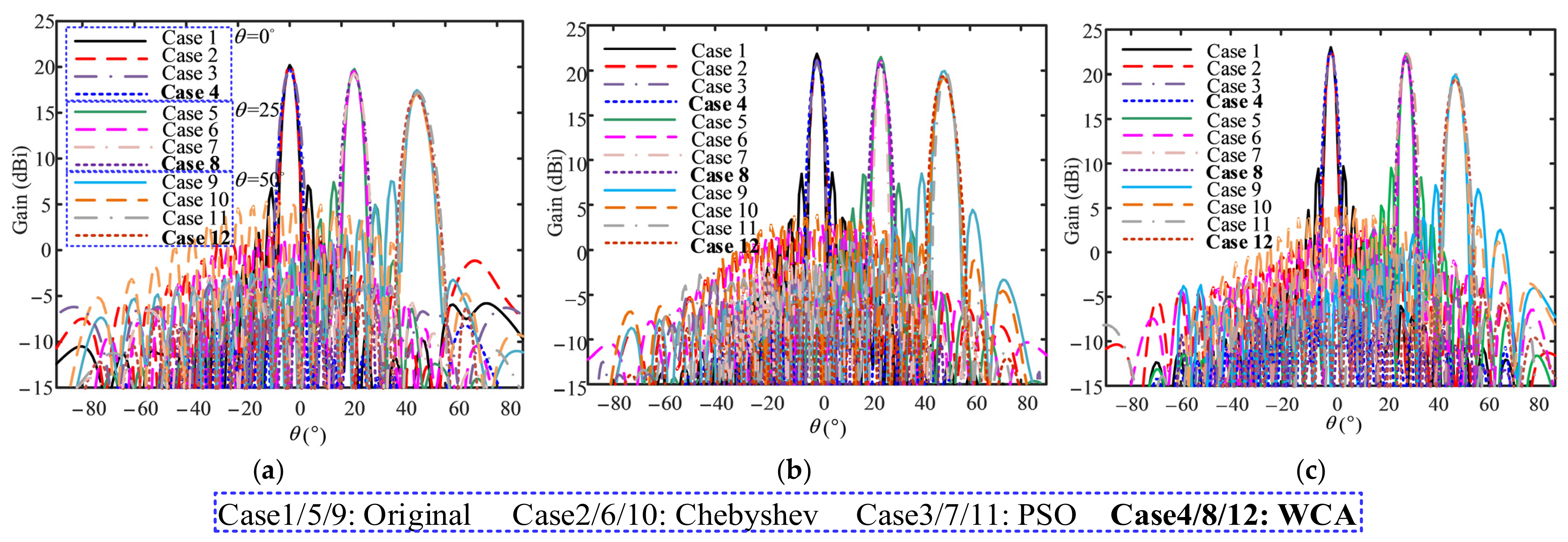
Figure 15.
Simulated beampatterns at (a) 2.5 GHz, (b) 3.0 GHz, and (c) 3.5 GHz under , and beam steering, where Cases 1–4 correspond to ; Cases 5–8 to ; Cases 9–12 to ; each group includes original, −20 dB Chebyshev-weighted, PSO- and WCA-synthesized patterns.
Figure 15.
Simulated beampatterns at (a) 2.5 GHz, (b) 3.0 GHz, and (c) 3.5 GHz under , and beam steering, where Cases 1–4 correspond to ; Cases 5–8 to ; Cases 9–12 to ; each group includes original, −20 dB Chebyshev-weighted, PSO- and WCA-synthesized patterns.
Table 1.
Benchmark functions.
Table 1.
Benchmark functions.
| Function Names | Expressions | Dimension(D) | Boundaries | Optimal Solution |
|---|
| Sphere function(F1) | | 10, 20, 30 | | |
| Schwefel’s Problem 2.22 (F2) | | 10, 20, 30 | | |
| Ackley’s Function (F3) | | 10, 20, 30 | | |
| Generalized Penalized Function (F4) |
where
and | 10, 20, 30 | | |
Table 2.
Comparisons of PSO, GA and WCA.
Table 2.
Comparisons of PSO, GA and WCA.
| Function | Dimension | Algorithm | Best | Worst | Mean | Std | Time(s) | Convergence Iter |
|---|
| F1 | 30 | PSO | 1.4 × 10⁻¹ | 3.9 × 10⁻¹ | 2.1 × 10⁻¹ | 5.0 × 10⁻² | 2.7375 | 989 |
| GA | 3.1 × 10⁻³ | 6.6 × 10⁻² | 2.2 × 10⁻² | 1.5 × 10⁻² | 2.9874 | 938 |
| WCA | 3.7 × 10⁻²⁰ | 2.0 × 10⁻¹⁴ | 1.3 × 10⁻¹⁵ | 3.8 × 10⁻¹⁵ | 1.0754 | 122 |
| F2 | 30 | PSO | 9.2 × 10⁻¹ | 1.6 × 100 | 1.4 × 100 | 1.7 × 10⁻¹ | 2.7418 | 778 |
| GA | 7.4 × 10⁻¹ | 4.7 × 100 | 1.9 × 100 | 8.6 × 10⁻¹ | 2.9937 | 971 |
| WCA | 5.4 × 10⁻¹¹ | 2.3 × 10⁻⁸ | 4.4 × 10⁻⁹ | 5.7 × 10⁻⁹ | 1.1503 | 167 |
| F3 | 30 | PSO | 1.3 × 100 | 1.8 × 100 | 1.6 × 100 | 1.4 × 10⁻¹ | 3.2154 | 659 |
| GA | 2.2 × 100 | 5.5 × 100 | 3.6 × 100 | 8.5 × 10⁻¹ | 3.2158 | 993 |
| WCA | 1.8 × 10⁻¹³ | 5.0 × 10⁻⁴ | 1.3 × 10⁻⁵ | 7.9 × 10⁻⁵ | 1.5203 | 305 |
| F4 | 30 | PSO | 1.8 × 100 | 1.9 × 100 | 1.9 × 100 | 1.6 × 10⁻² | 3.8280 | 893 |
| GA | 9.5 × 10⁻⁷ | 8.3 × 10⁻¹ | 1.1 × 10⁻¹ | 2.1 × 10⁻¹ | 3.8832 | 881 |
| WCA | 5.8 × 10⁻²¹ | 1.0 × 10⁻² | 2.6 × 10⁻³ | 2.6 × 10⁻² | 2.0306 | 186 |
Table 3.
Searching space of E-shaped patch antenna.
Table 3.
Searching space of E-shaped patch antenna.
| Parameters | Wp | Lp | Ws |
| Min (mm) | 10 | 10 | 0.5 |
| Max (mm) | 50 | 30 | Wp/2 |
| Parameters | Ls | Px | Py |
| Min (mm) | 0.5 | −Lp/2 | Ws/2 |
| Max (mm) | Lp | Lp/2 | Wp/2−Ws/2 |
Table 4.
Optimized parameters of E-shaped patch antenna.
Table 4.
Optimized parameters of E-shaped patch antenna.
| Parameters | Wp | Lp | Ws | Ls | Px | Py |
|---|
| Values(mm) | 49.79 | 20.29 | 2.47 | 17.49 | 4.96 | 6.77 |
Table 5.
Results comparison for the design of the E-shaped patch antenna with different methods.
Table 5.
Results comparison for the design of the E-shaped patch antenna with different methods.
| Ref. | Methods | Max.S11 (dB) | BW (%) |
|---|
| [4] | GWO | −34.59 | 26.73 |
| [20] | DE | −30.48 | 20.55 |
| [20] | SaDE | −34.06 | 20.18 |
| [28] | WDO | −31.00 | 20.00 |
| Prop. | WCA | −37.18 | 28.41 |
Table 6.
Statistical performance of the WCA for the E-shaped patch antenna.
Table 6.
Statistical performance of the WCA for the E-shaped patch antenna.
| Metric | Best | Worst | Mean | Std |
|---|
| Max.S11 (dB) | −37.18 | −26.26 | −34.72 | 2.24 |
| Bandwidth (%) | 28.41 | 26.35 | 27.68 | 0.48 |
Table 7.
Searching space of the ME dipole antenna.
Table 7.
Searching space of the ME dipole antenna.
| Parameters | W | L | H | a | b | c | d | e |
|---|
| Min (mm) | 30 | 10 | 10 | 4.5 | 12 | 0.5 | 2 | 1.5 |
| Max (mm) | 90 | 50 | 50 | 14.5 | 32 | 5 | 8 | 11.5 |
Table 8.
Optimized parameters of the conventional ME dipole antenna.
Table 8.
Optimized parameters of the conventional ME dipole antenna.
| Parameters | W | L | H | a | b |
| Values (mm) | 53.57 | 27.77 | 27.20 | 10.53 | 14.34 |
| Parameters | c | d | e | S | |
| Values (mm) | 1.89 | 5.68 | 1.93 | 14.35 | |
Table 9.
Statistical performance of the WCA for the conventional ME dipole antenna.
Table 9.
Statistical performance of the WCA for the conventional ME dipole antenna.
| Metric | Best | Worst | Mean | Std |
|---|
| Max. VSWR | 1.45 | 1.49 | 1.47 | 0.02 |
| Bandwidth (%) | 80.9 | 78.5 | 79.5 | 0.76 |
Table 10.
Results comparison for the design of ME dipole antenna with different methods.
Table 10.
Results comparison for the design of ME dipole antenna with different methods.
| Ref. | Method | Parameters (mm) | Antenna Size | BW (%)
(VSWR ≤ 1.5) |
|---|
| W | L | H | S |
|---|
| [38] | HFSS | 60 | 30 | 30.0 | 17 | 0.50λ × 0.64λ × 0.250λ | 43.8 |
| [4] | GWO | 74.23 | 28.01 | 27.91 | 15.76 | 0.62λ × 0.60λ × 0.233λ | 80.0 |
| Prop. | WCA | 53.57 | 27.77 | 27.20 | 14.35 | 0.45λ × 0.58λ × 0.227λ | 80.9 |
Table 11.
Searching space of the proposed ME dipole antenna.
Table 11.
Searching space of the proposed ME dipole antenna.
| Parameters | R | L | H | a | b | c | d | e |
|---|
| Min (mm) | 15 | 10 | 10 | 4.5 | 12 | 0.5 | 2 | 1.5 |
| Max (mm) | 45 | 30 | 50 | 14.5 | 32 | 5 | 8 | 11.5 |
Table 12.
Optimized dimensions of bandwidth-enhanced ME dipole.
Table 12.
Optimized dimensions of bandwidth-enhanced ME dipole.
| Parameters | R | L | H | a | b |
| Values (mm) | 24.31 | 20.67 | 26.36 | 12.26 | 12.04 |
| Parameters | c | d | e | S | / |
| Values (mm) | 1.93 | 5.11 | 2.2 | 16.39 | / |
Table 13.
Performance comparison between the proposed and reported ME dipole antennas.
Table 13.
Performance comparison between the proposed and reported ME dipole antennas.
| Ref. | Structure | Ave. Gain (dBi) | BW (%)
(VSWR ≤ 2) |
|---|
| [39] | Complex | 6.0 | 61.6 |
| [40] | Simple | 10.0 | 53.0 |
| [41] | Simple | 8.0 | 85.0 |
| [42] | Simple | 7.2 | 86.9 |
| Prop. | Simple | 8.0 | 92.4 |
Table 14.
Statistical performance of the WCA for the bandwidth-enhanced ME dipole antenna.
Table 14.
Statistical performance of the WCA for the bandwidth-enhanced ME dipole antenna.
| Metric | Best | Worst | Mean | Std |
|---|
| Max. VSWR | 1.65 | 1.90 | 1.76 | 0.08 |
| Bandwidth (%) | 92.4 | 89.1 | 90.7 | 0.90 |
Table 15.
Gains and SLLs of beampatterns at 2.5 GHz in the above 12 cases.
Table 15.
Gains and SLLs of beampatterns at 2.5 GHz in the above 12 cases.
| Cases | Gain (dBi) | SLL (dB) | Cases | Gain (dBi) | SLL (dB) |
|---|
| Case 1 | 20.3 | −13.6 | Case 7 | 19.3 | −23.2 |
| Case 2 | 20.2 | −18.4 | Case 8 | 19.2 | −26.0 |
| Case 3 | 20.0 | −24.3 | Case 9 | 17.2 | −9.8 |
| Case 4 | 19.8 | −27.9 | Case 10 | 16.8 | −12.4 |
| Case 5 | 19.7 | −12.3 | Case 11 | 16.6 | −18.6 |
| Case 6 | 19.5 | −16.2 | Case 12 | 16.4 | −20.1 |
Table 16.
Gains and SLLs of beampatterns at 3.0 GHz in the above 12 cases.
Table 16.
Gains and SLLs of beampatterns at 3.0 GHz in the above 12 cases.
| Cases | Gain (dBi) | SLL (dB) | Cases | Gain (dBi) | SLL (dB) |
|---|
| Case 1 | 21.9 | −14.3 | Case 7 | 20.9 | −25.6 |
| Case 2 | 21.6 | −19.7 | Case 8 | 20.7 | −27.2 |
| Case 3 | 21.5 | −24.1 | Case 9 | 19.7 | −11.5 |
| Case 4 | 21.3 | −29.3 | Case 10 | 19.3 | −15.4 |
| Case 5 | 21.3 | −13.1 | Case 11 | 19.2 | −21.3 |
| Case 6 | 21.0 | −18.2 | Case 12 | 19.0 | −23.8 |
Table 17.
Gains and SLLs of beampatterns at 3.5 GHz in the above 12 cases.
Table 17.
Gains and SLLs of beampatterns at 3.5 GHz in the above 12 cases.
| Cases | Gain (dBi) | SLL (dB) | Cases | Gain (dBi) | SLL (dB) |
|---|
| Case 1 | 24.1 | −13.6 | Case 7 | 22.1 | −25.8 |
| Case 2 | 22.8 | −19.2 | Case 8 | 21.9 | −27.9 |
| Case 3 | 22.6 | −27.4 | Case 9 | 20.0 | −12.6 |
| Case 4 | 22.5 | −30.0 | Case 10 | 18.4 | −14.5 |
| Case 5 | 22.4 | −12.9 | Case 11 | 19.6 | −20.2 |
| Case 6 | 22.2 | −17.9 | Case 12 | 19.3 | −22.9 |
Table 18.
Computational time and convergence iteration comparison at θ = 0°.
Table 18.
Computational time and convergence iteration comparison at θ = 0°.
| Frequency (GHz) | Algorithm | Time(s) | Convergence Iterations |
|---|
| 2.5 | PSO | 1.78 | 500 |
| WCA | 0.89 | 258 |
| 3.0 | PSO | 1.82 | 497 |
| WCA | 0.65 | 253 |
| 3.5 | PSO | 1.86 | 502 |
| WCA | 1.08 | 268 |