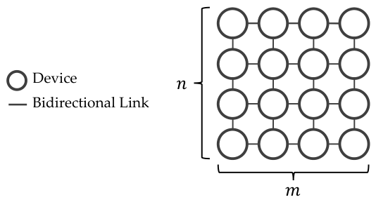
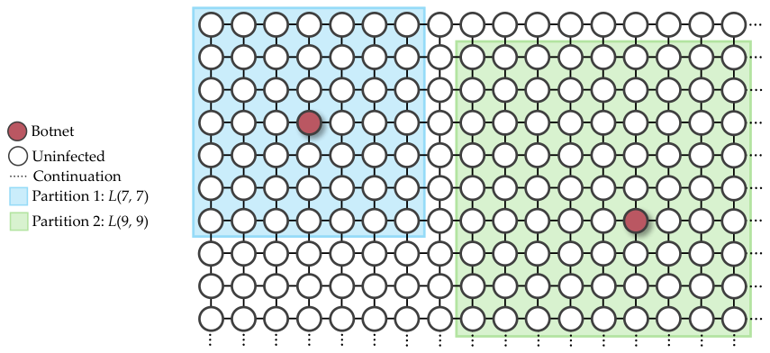
Figure 1.
A grid topology network is defined as a network in which devices are positioned at the vertices, and the connections between neighboring vertices are bidirectional links.
Figure 1.
A grid topology network is defined as a network in which devices are positioned at the vertices, and the connections between neighboring vertices are bidirectional links.
Figure 2.
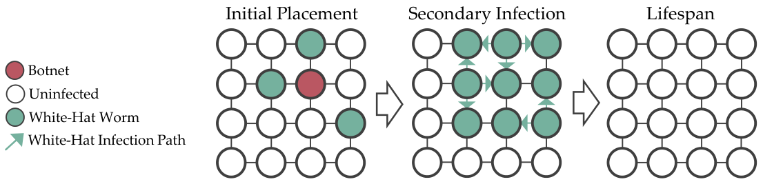
A white-hat worm is defined by its ability to cause secondary infections that reinfect and eliminate botnets from devices, and it also has a lifespan that allows it to delete itself.
Figure 2.
A white-hat worm is defined by its ability to cause secondary infections that reinfect and eliminate botnets from devices, and it also has a lifespan that allows it to delete itself.
Figure 3.
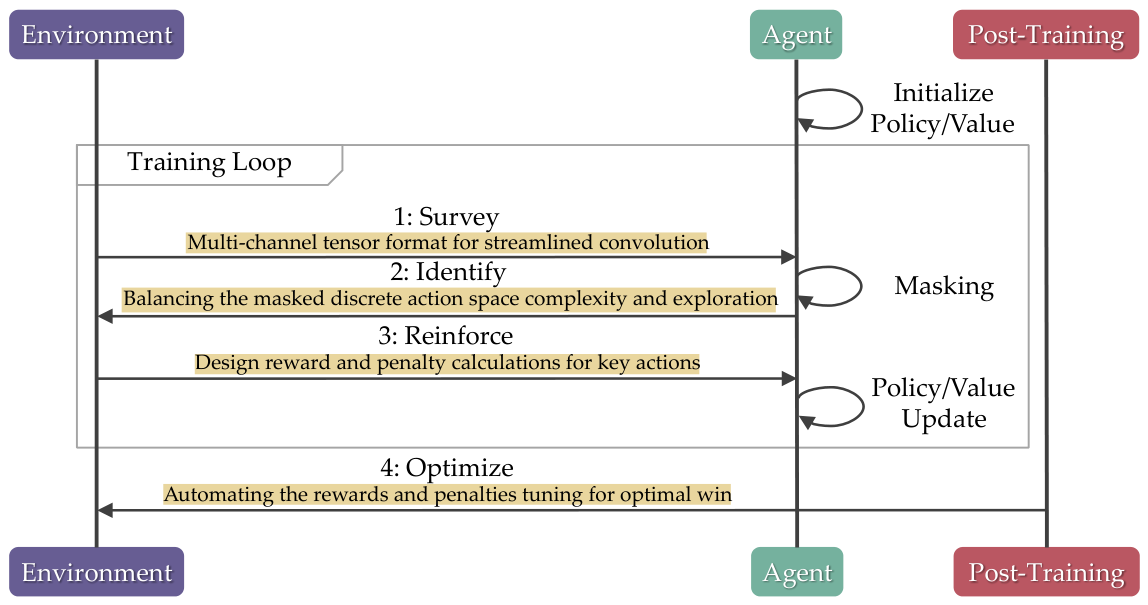
The framework augments the typical reinforcement learning workflow to ensure wider compatibility across different algorithms.
Figure 3.
The framework augments the typical reinforcement learning workflow to ensure wider compatibility across different algorithms.
Figure 4.
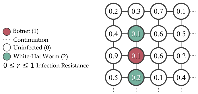
The simulation expresses the infection resistance as a decimal between 0 and 1, with uninfected devices represented as 0, botnets as 1, and white-hat worms as 2.
Figure 4.
The simulation expresses the infection resistance as a decimal between 0 and 1, with uninfected devices represented as 0, botnets as 1, and white-hat worms as 2.
Figure 5.
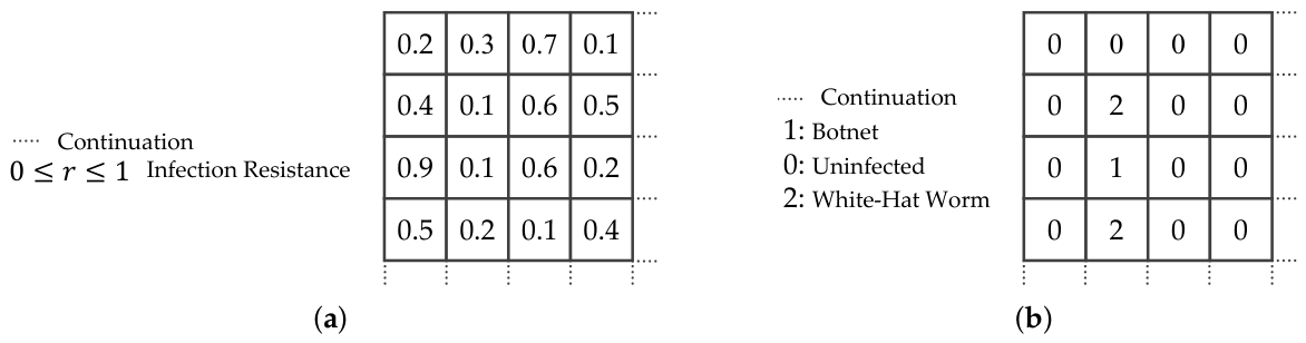
(a) A 2D array is used to represent the infection resiliency of each device. (b) Another 2D array is used to represent the infection state of each device.
Figure 5.
(a) A 2D array is used to represent the infection resiliency of each device. (b) Another 2D array is used to represent the infection state of each device.
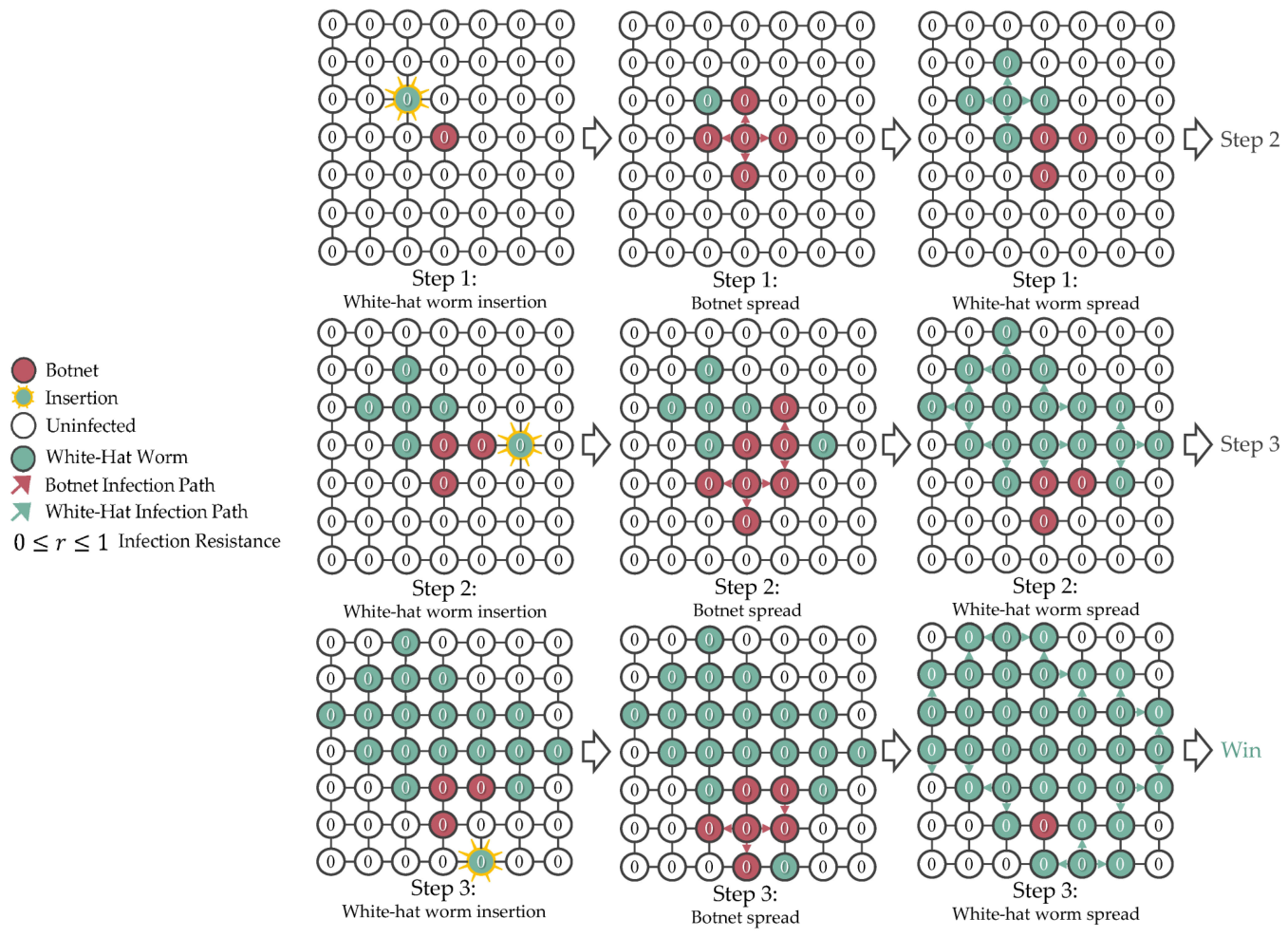
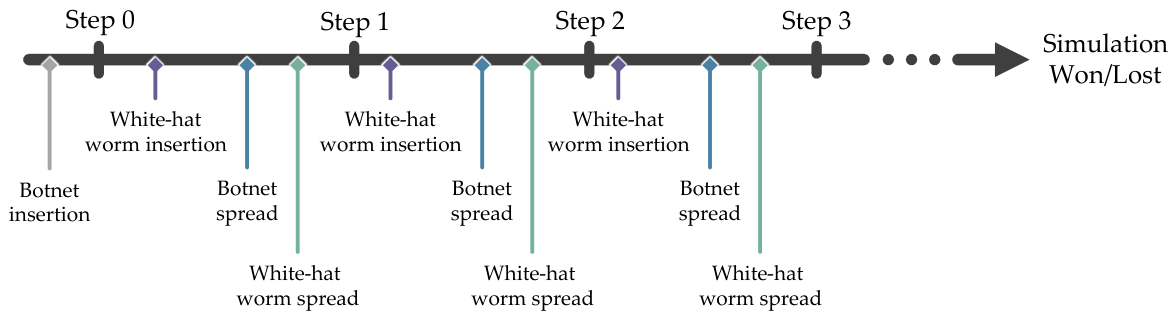
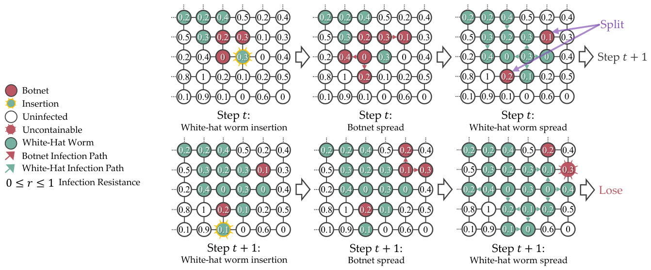
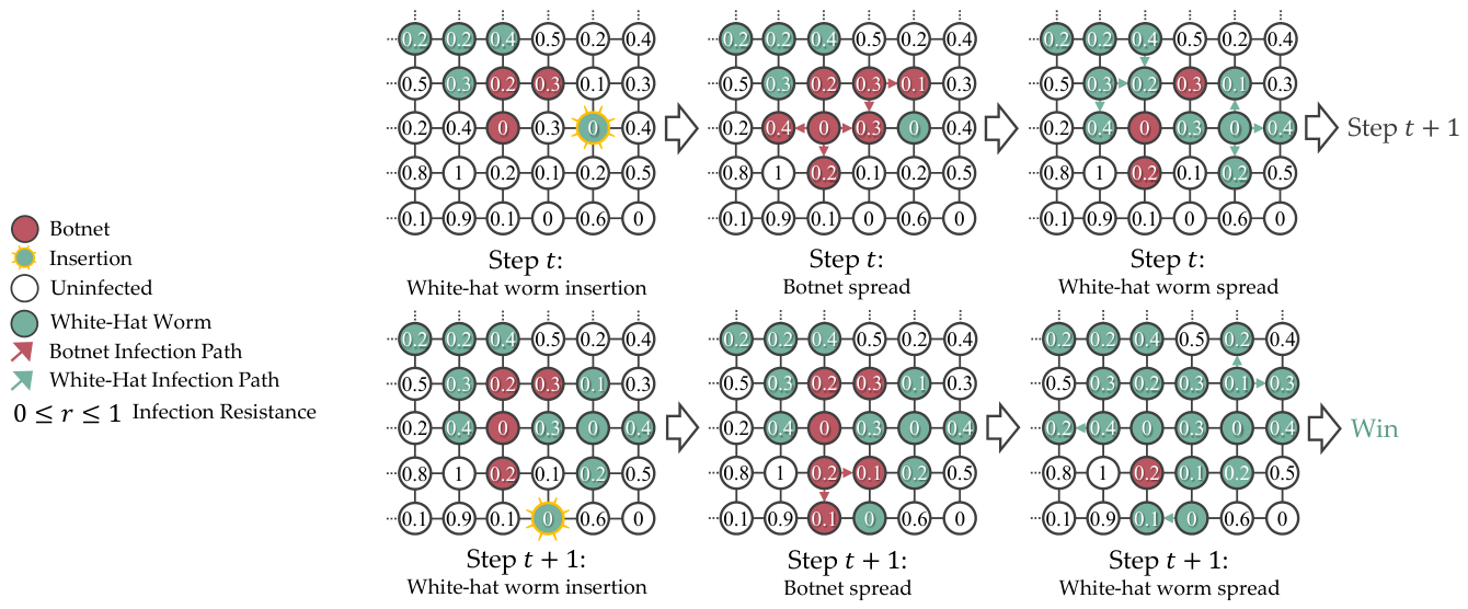
Figure 6.
The insertion and infection spread in the simulation are predetermined to maintain determinism for debugging and evaluation. The ellipsis indicates continuation.
Figure 6.
The insertion and infection spread in the simulation are predetermined to maintain determinism for debugging and evaluation. The ellipsis indicates continuation.
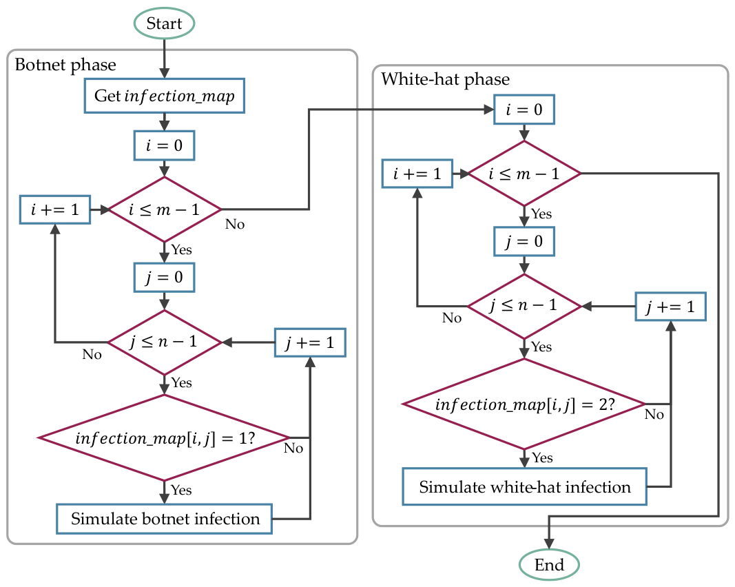
Figure 7.
The process for simulating the botnets’ and white-hat worms’ infection in a grid topology network for every timestep.
Figure 7.
The process for simulating the botnets’ and white-hat worms’ infection in a grid topology network for every timestep.
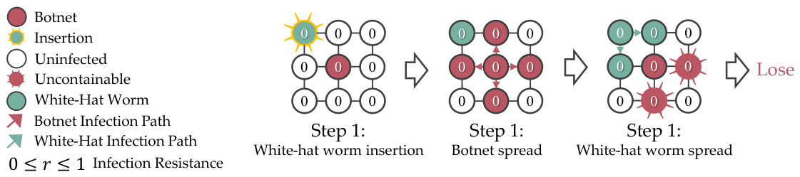
Figure 8.
Unresolvable simulation with the botnet starting one step from the grid boundary.
Figure 8.
Unresolvable simulation with the botnet starting one step from the grid boundary.
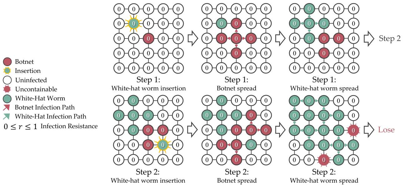
Figure 9.
Unresolvable simulation with the botnet starting two steps from the grid boundary.
Figure 9.
Unresolvable simulation with the botnet starting two steps from the grid boundary.
Figure 10.
Resolvable simulation with the botnet starting three steps from the grid boundary.
Figure 10.
Resolvable simulation with the botnet starting three steps from the grid boundary.
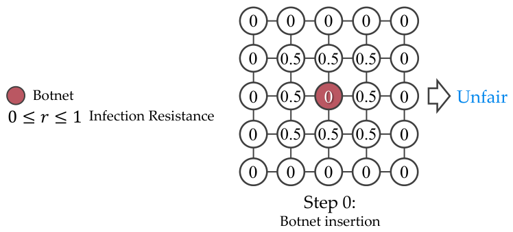
Figure 11.
Unfair simulation where botnet was surrounded by uninfectable devices () at step 0.
Figure 11.
Unfair simulation where botnet was surrounded by uninfectable devices () at step 0.
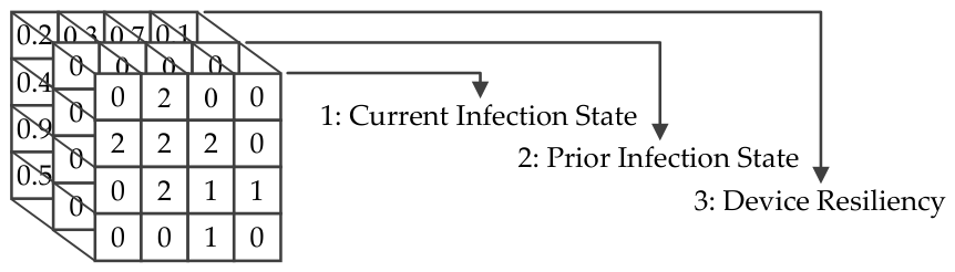
Figure 12.
A multi-channel tensor is used to represent the current infection state, the prior infection state, and the infection resiliency of each device.
Figure 12.
A multi-channel tensor is used to represent the current infection state, the prior infection state, and the infection resiliency of each device.
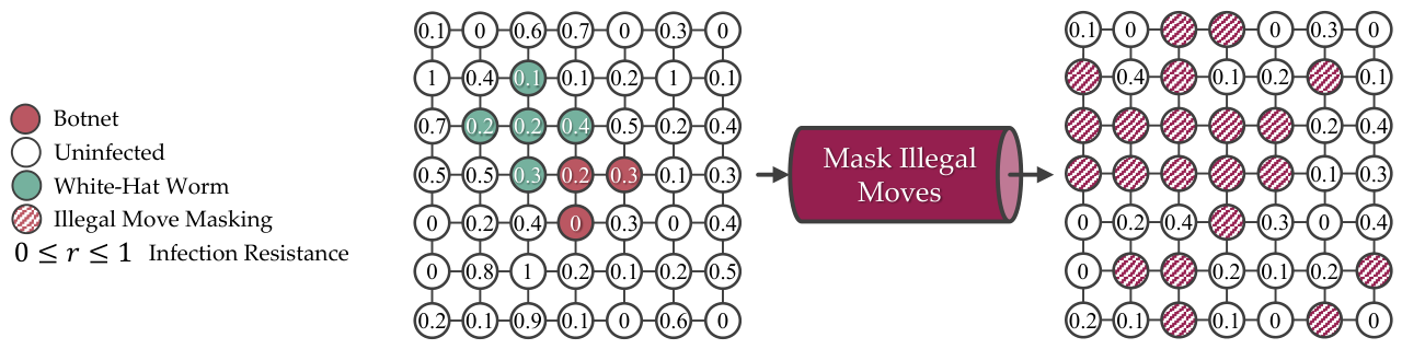
Figure 13.
Using a comparison operator to mask illegal moves reduces the complexity in discrete action space on the grid.
Figure 13.
Using a comparison operator to mask illegal moves reduces the complexity in discrete action space on the grid.
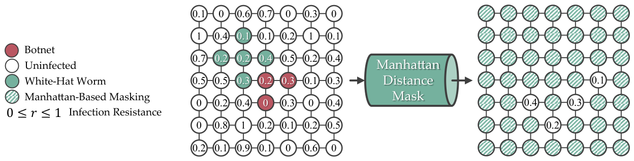
Figure 14.
Using a Manhattan-based masking strategy further reduces the complexity, at the cost of preventing the agent from exploring different winning strategies on the grid.
Figure 14.
Using a Manhattan-based masking strategy further reduces the complexity, at the cost of preventing the agent from exploring different winning strategies on the grid.
Figure 15.
The white-hat worm placed using the Manhattan-based masking strategy could cause the botnet infection trajectory to split on the grid, which makes containment impossible.
Figure 15.
The white-hat worm placed using the Manhattan-based masking strategy could cause the botnet infection trajectory to split on the grid, which makes containment impossible.
Figure 16.
Using a Chebyshev distance of 1 to detect infectable neighboring devices slightly reduces the complexity, allowing the agent to explore different winning strategies on .
Figure 16.
Using a Chebyshev distance of 1 to detect infectable neighboring devices slightly reduces the complexity, allowing the agent to explore different winning strategies on .
Figure 17.
The white-hat worm placed using a Chebyshev-based masking strategy could block multiple paths when the white-hat worm spread, effectively containing the botnets.
Figure 17.
The white-hat worm placed using a Chebyshev-based masking strategy could block multiple paths when the white-hat worm spread, effectively containing the botnets.
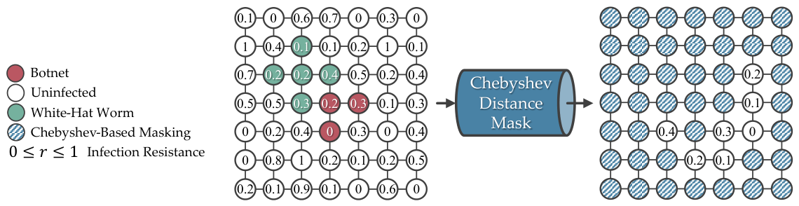
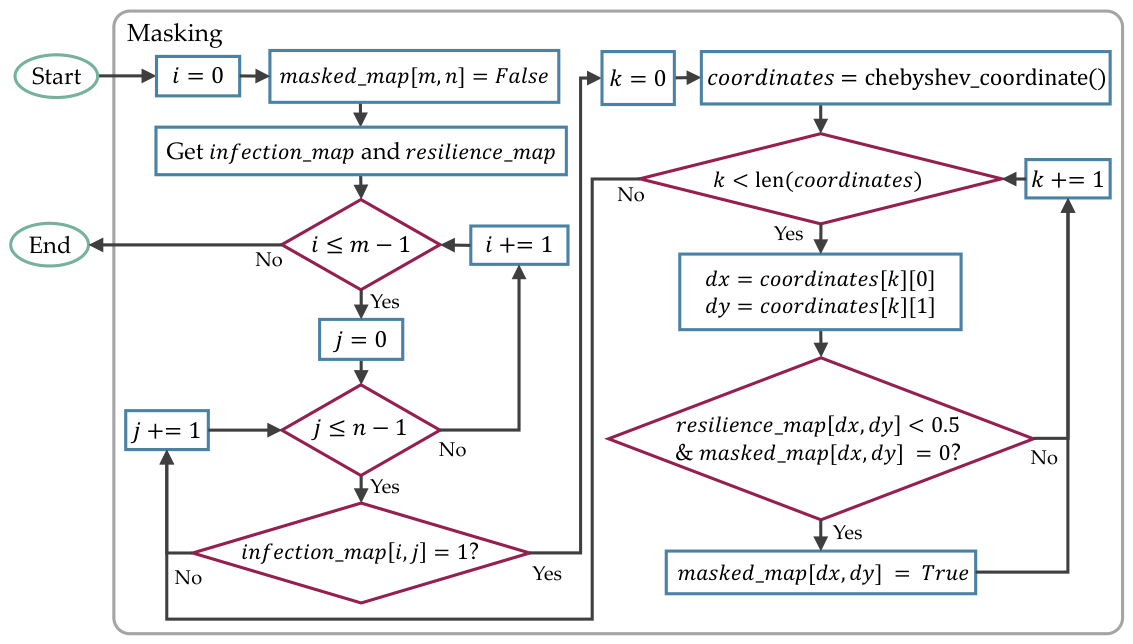
Figure 18.
The process for masking the devices relies on a Chebyshev-based masking strategy to identify infection paths that need to be blocked.
Figure 18.
The process for masking the devices relies on a Chebyshev-based masking strategy to identify infection paths that need to be blocked.
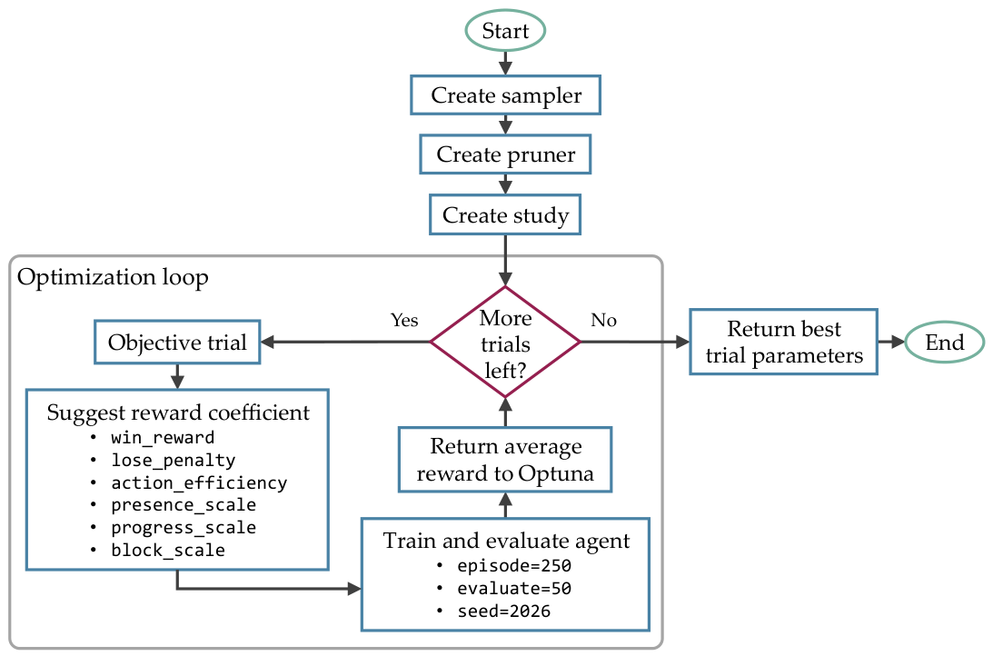
Figure 19.
The process to optimize the reward and penalty coefficients utilized Optuna to tune the , , , , , and .
Figure 19.
The process to optimize the reward and penalty coefficients utilized Optuna to tune the , , , , , and .
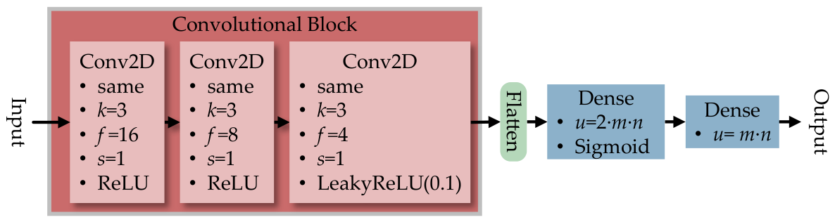
Figure 20.
The convolutional neural network-based encoder model is used on all reinforcement learning algorithms for consistency in analyzing the grid-topology network.
Figure 20.
The convolutional neural network-based encoder model is used on all reinforcement learning algorithms for consistency in analyzing the grid-topology network.
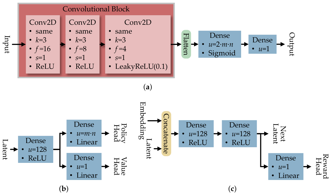
Figure 21.
(a) The convolutional neural network-based encoder is used as the critic network in proximal policy optimization. (b) The multi-task prediction network is used to predict the next hidden state and reward in MuZero. (c) The multi-task dynamic network is used to estimate the policy and value of a hidden state in MuZero.
Figure 21.
(a) The convolutional neural network-based encoder is used as the critic network in proximal policy optimization. (b) The multi-task prediction network is used to predict the next hidden state and reward in MuZero. (c) The multi-task dynamic network is used to estimate the policy and value of a hidden state in MuZero.
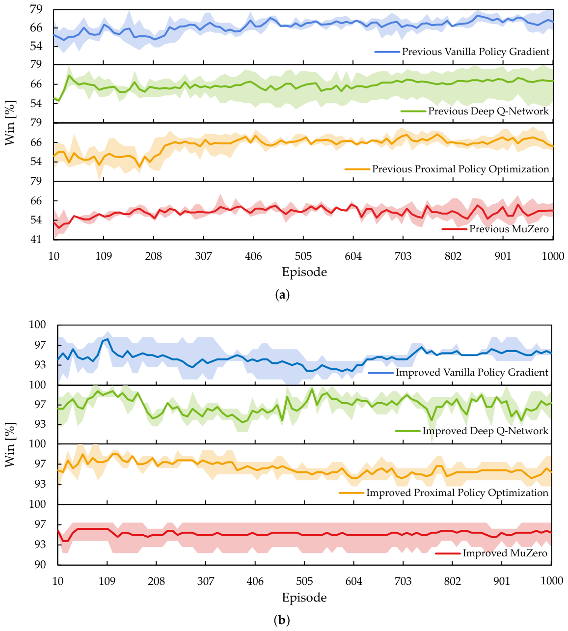
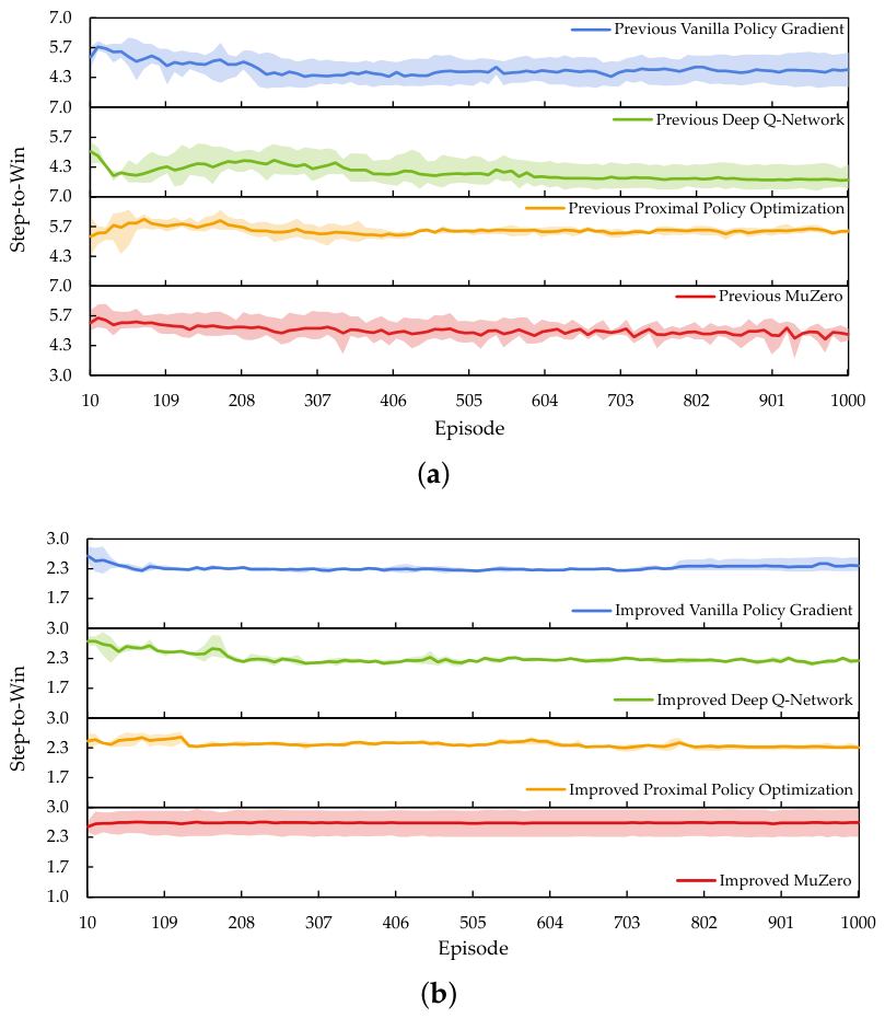
Figure 22.
The mean line plot with minimum and maximum values as a range band on the winning rate. (a) Most of the agents configured with the previous reinforcement learning setup improve slowly and plateau below a 80% winning rate. (b) The agents improved with the survey–identify–reinforce–optimize framework exceeded 90%, with some achieving a 100% winning rate.
Figure 22.
The mean line plot with minimum and maximum values as a range band on the winning rate. (a) Most of the agents configured with the previous reinforcement learning setup improve slowly and plateau below a 80% winning rate. (b) The agents improved with the survey–identify–reinforce–optimize framework exceeded 90%, with some achieving a 100% winning rate.
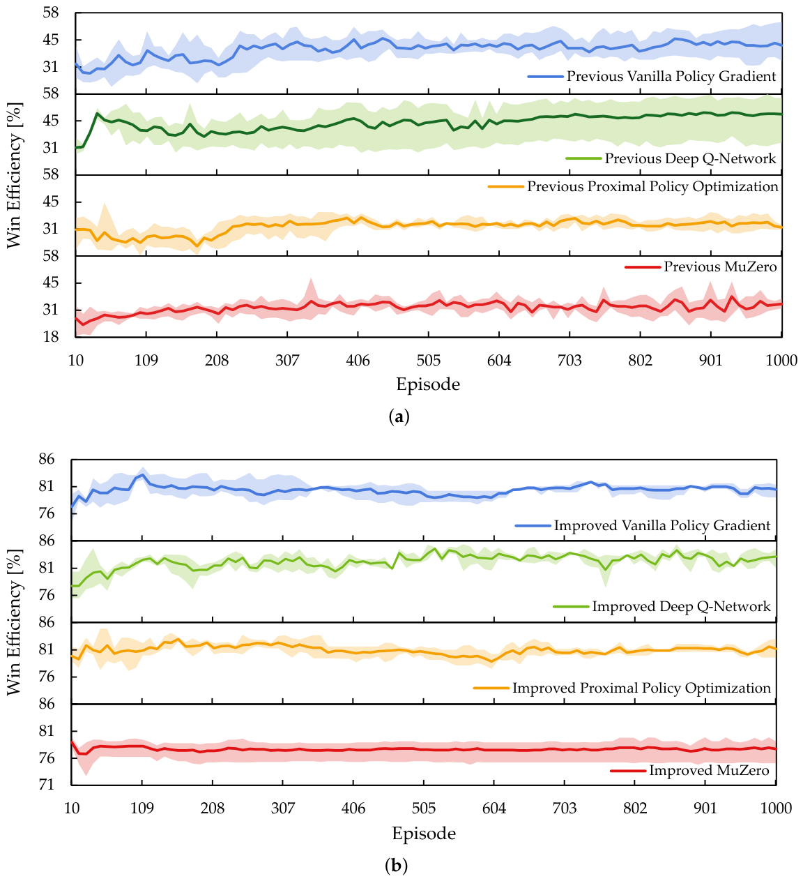
Figure 23.
The mean line plot with minimum and maximum values as a range band on the win efficiency. (a) The agents that are configured using the previous reinforcement learning setup struggle to improve their win efficiency beyond 60%. (b) The agents improved with the survey–identify–reinforce–optimize framework, maintaining a mean win efficiency above 70%.
Figure 23.
The mean line plot with minimum and maximum values as a range band on the win efficiency. (a) The agents that are configured using the previous reinforcement learning setup struggle to improve their win efficiency beyond 60%. (b) The agents improved with the survey–identify–reinforce–optimize framework, maintaining a mean win efficiency above 70%.
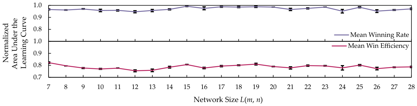
Figure 24.
The plotted area under the learning curves for the deep Q-network agent shows slight improvement as the network size increases, before oscillating on onward.
Figure 24.
The plotted area under the learning curves for the deep Q-network agent shows slight improvement as the network size increases, before oscillating on onward.
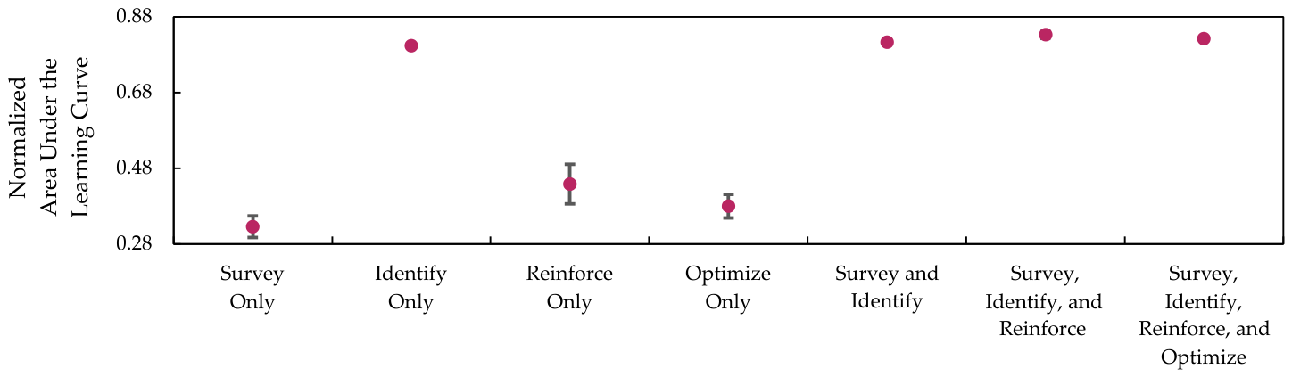
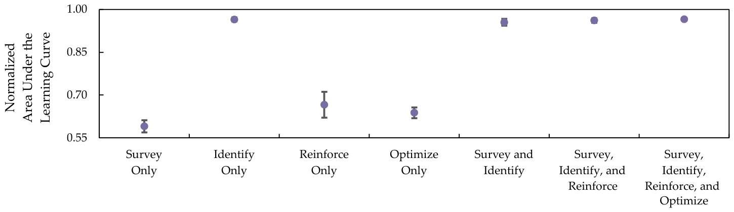
Figure 25.
The winning rate is represented by the mean and normalized area under the learning curves, with error bars indicating the standard deviation of each component.
Figure 25.
The winning rate is represented by the mean and normalized area under the learning curves, with error bars indicating the standard deviation of each component.
Figure 26.
The win efficiency is represented by the mean and normalized area under the learning curves, with error bars indicating the standard deviation of each component.
Figure 26.
The win efficiency is represented by the mean and normalized area under the learning curves, with error bars indicating the standard deviation of each component.
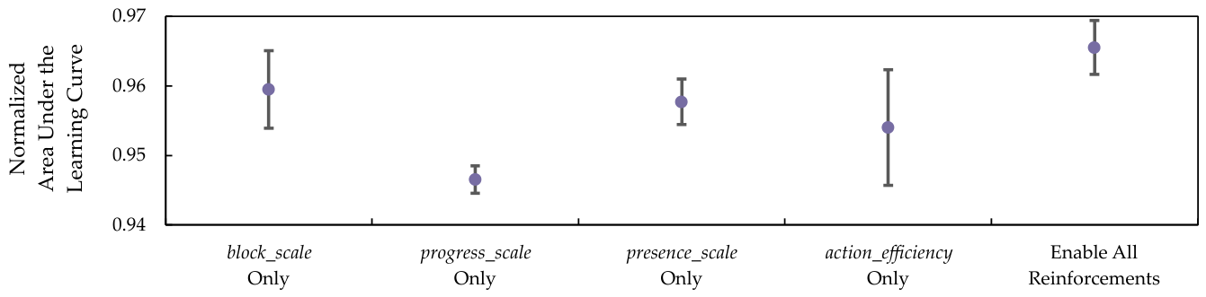
Figure 27.
The winning rate is represented by the mean and normalized area under the learning curves, with error bars indicating the standard deviation of each reinforcement.
Figure 27.
The winning rate is represented by the mean and normalized area under the learning curves, with error bars indicating the standard deviation of each reinforcement.
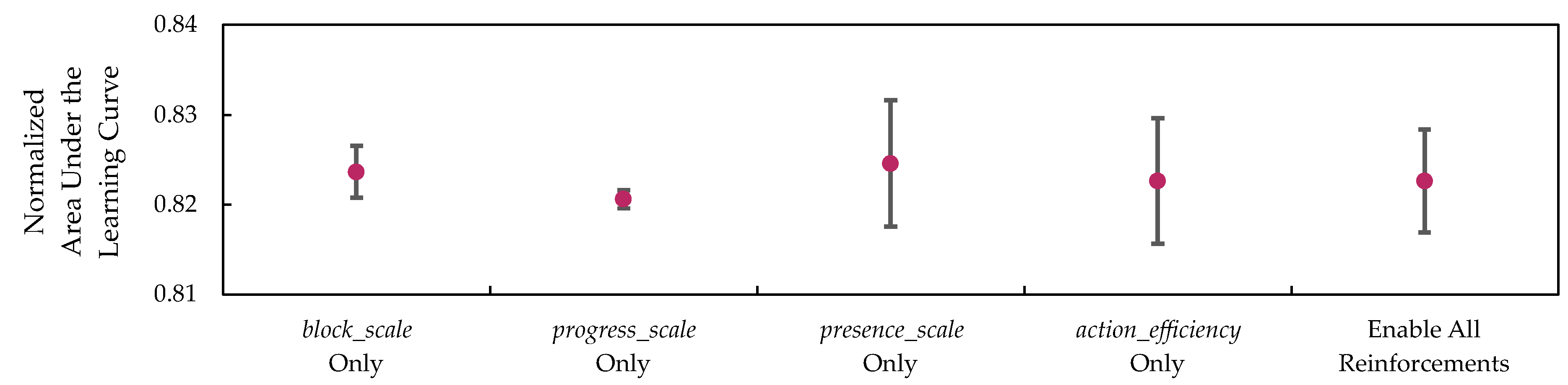
Figure 28.
The win efficiency is represented by the mean and normalized area under the learning curves, with error bars indicating the standard deviation of each reinforcement.
Figure 28.
The win efficiency is represented by the mean and normalized area under the learning curves, with error bars indicating the standard deviation of each reinforcement.
Figure 29.
To scale beyond the grid topology network it was not trained with and , grid partitioning is recommended for generalization.
Figure 29.
To scale beyond the grid topology network it was not trained with and , grid partitioning is recommended for generalization.
Table 1.
Existing research that requires specific conditions and high-quality datasets to be effective against the framework proposed in this article.
Table 1.
Existing research that requires specific conditions and high-quality datasets to be effective against the framework proposed in this article.
| Authors | Device
Immunity | Network
Topology | Benign
Worms | White-Hat Worm Launcher |
|---|
| Bulk | Timestep |
|---|
| Muthukumar et al. [8] | ✓ | | | | |
| Rodríguez et al. [9] | | ✓ | | | |
| Asadi et al. [10] | ✓ | | ✓ | | |
| Okawa et al. [11] | ✓ | | | | |
| Tatebatake et al. [12] | | ✓ | | | |
| Jia et al. [13] | | | ✓ | | |
| Pan et al. [14] | | | | ✓ | |
| Yoshioka et al. [16] | | | | | ✓* |
| This article | | | | | ✓ |
Table 2.
The reinforcement learning algorithms used to evaluate the effectiveness of the proposed framework.
Table 2.
The reinforcement learning algorithms used to evaluate the effectiveness of the proposed framework.
| Algorithm | Model | Data | Optimization | Planning |
|---|
| Vanilla policy gradient | Model-free | On-policy | Policy-gradient | No |
| Deep Q-network | Model-free | Off-policy | Q-learning | No |
| Proximal policy optimization | Model-free | On-policy | Actor-critic | No |
| MuZero | Model-based | Off-policy | Policy, value, and model | Yes |
Table 3.
The hand-tuned hyperparameter values for the scales are used to obtain the episodic and step-based reinforcement, with a positive sign for rewards and a negative sign for penalties.
Table 3.
The hand-tuned hyperparameter values for the scales are used to obtain the episodic and step-based reinforcement, with a positive sign for rewards and a negative sign for penalties.
| Scale | Sign | Value | Type |
|---|
| + | 0.05 | Reward |
| + | 0.5 | Reward |
| − | 1 | Penalty |
| − | 0.005 | Penalty |
| + | 0.2 | Reward |
| + | 0.5 | Reward |
Table 4.
The reward and penalty value ranges used by Optuna to identify the optimal reward coefficient over 30 trials, with a positive sign for rewards and a negative sign for penalties.
Table 4.
The reward and penalty value ranges used by Optuna to identify the optimal reward coefficient over 30 trials, with a positive sign for rewards and a negative sign for penalties.
| Scale | Sign | Value Range | Type |
|---|
| + | 0–0.2 | Reward |
| + | 0.1–2 | Reward |
| − | 0.5–2 | Penalty |
| − | 0–0.05 | Penalty |
| + | 0–1 | Reward |
| + | 0.1–1 | Reward |
Table 5.
The hyperparameters used to configure the vanilla policy gradient.
Table 5.
The hyperparameters used to configure the vanilla policy gradient.
| Vanilla Policy Gradient’s Hyperparameters | Value |
|---|
| Gamma | 0.99 |
| Batch size | 64 |
| Epoch number | 10 |
| Adam’s learning rate | 0.0003 |
Table 6.
The hyperparameters used to configure the deep Q-network.
Table 6.
The hyperparameters used to configure the deep Q-network.
| Deep Q-network’s Hyperparameters | Value |
|---|
| Epsilon | 1 |
| Gamma | 0.99 |
| Batch size | 64 |
| Memory size | 100,000 |
| Epsilon decay | 0.995 |
| Update interval | 1000 |
| Minimum epsilon | 0.05 |
| Adam’s learning rate | 0.0003 |
Table 7.
The hyperparameters used to configure the proximal policy optimization.
Table 7.
The hyperparameters used to configure the proximal policy optimization.
| Proximal Policy Optimization’s Hyperparameters | Value |
|---|
| Gamma | 0.99 |
| Batch size | 64 |
| Policy clip | 0.2 |
| Epoch number | 10 |
| Adam’s learning rate | 0.0003 |
| Generalized advantage estimation | 0.95 |
Table 8.
The hyperparameters used to configure the MuZero.
Table 8.
The hyperparameters used to configure the MuZero.
| MuZero’s Hyperparameters | Value |
|---|
| Gamma | 0.8 |
| Unroll steps | 5 |
| Latent dimension | 128 |
| Maximum memory | 50,000 |
| Adam’s learning rate | 0.001 |
| Number of simulation | 10 |
| Maximum episodes kept | 2000 |
| Embedded action dimension | 32 |
| Predictor-based upper confidence tree constant | 1 |
Table 9.
The normalized area under the learning curve for winning rate with standard deviation across different reinforcement learning agent implementations.
Table 9.
The normalized area under the learning curve for winning rate with standard deviation across different reinforcement learning agent implementations.
| Algorithm | Implementation | Mean | Standard Deviation |
|---|
| Vanilla policy gradient | Previous | 0.6765 | 0.0206 |
| Improved | 0.9456 | 0.0129 |
| Deep Q-network | Previous | 0.6581 | 0.0815 |
| Improved | 0.9655 | 0.0039 |
| Proximal policy optimization | Previous | 0.6476 | 0.0098 |
| Improved | 0.9601 | 0.0041 |
| MuZero | Previous | 0.5885 | 0.0149 |
| Improved | 0.9521 | 0.0212 |
Table 10.
The normalized area under the learning curve for win efficiency with standard deviation across different reinforcement learning agent implementations.
Table 10.
The normalized area under the learning curve for win efficiency with standard deviation across different reinforcement learning agent implementations.
| Algorithm | Implementation | Mean | Standard Deviation |
|---|
| Vanilla policy gradient | Previous | 0.4001 | 0.0547 |
| Improved | 0.8037 | 0.0065 |
| Deep Q-network | Previous | 0.4386 | 0.0931 |
| Improved | 0.8226 | 0.0057 |
| Proximal policy optimization | Previous | 0.3253 | 0.0069 |
| Improved | 0.8094 | 0.0047 |
| MuZero | Previous | 0.3263 | 0.0348 |
| Improved | 0.7764 | 0.0200 |
Table 11.
The mean percentage change for the area under the learning curve on winning rate and win efficiency.
Table 11.
The mean percentage change for the area under the learning curve on winning rate and win efficiency.
| Algorithm | Winning Rate Improvement [%] | Win Efficiency Improvement [%] |
|---|
| Vanilla policy gradient | 39.7780 | 100.8822 |
| Deep Q-network | 46.7129 | 87.5708 |
| Proximal policy optimization | 48.2453 | 148.8404 |
| MuZero | 61.7809 | 137.9191 |
| Mean | 49.1293 | 118.8031 |
Table 12.
The area under the learning curves for the deep Q-network agent slightly improves as the network size increases, before oscillating on and onward.
Table 12.
The area under the learning curves for the deep Q-network agent slightly improves as the network size increases, before oscillating on and onward.
Network Size
| Winning Rate | Win Efficiency |
|---|
| Mean | Standard Deviation | Mean | Standard Deviation |
|---|
| 7 | 0.9655 | 0.0039 | 0.8226 | 0.0057 |
| 8 | 0.9611 | 0.0016 | 0.7961 | 0.0006 |
| 9 | 0.9697 | 0.0026 | 0.7773 | 0.0045 |
| 10 | 0.9571 | 0.0106 | 0.7701 | 0.0042 |
| 11 | 0.9577 | 0.0053 | 0.7771 | 0.0011 |
| 12 | 0.9463 | 0.0082 | 0.7544 | 0.0077 |
| 13 | 0.9566 | 0.0098 | 0.7588 | 0.0107 |
| 14 | 0.9671 | 0.0048 | 0.7842 | 0.0076 |
| 15 | 0.9926 | 0.0045 | 0.8064 | 0.0025 |
| 16 | 0.9753 | 0.0115 | 0.7776 | 0.0063 |
| 17 | 0.9875 | 0.0044 | 0.7934 | 0.0055 |
| 18 | 0.9858 | 0.0052 | 0.8008 | 0.0032 |
| 19 | 0.9887 | 0.0063 | 0.8109 | 0.0074 |
| 20 | 0.9854 | 0.0012 | 0.7901 | 0.0024 |
| 21 | 0.9657 | 0.0096 | 0.7786 | 0.0093 |
| 22 | 0.9750 | 0.0048 | 0.7978 | 0.0052 |
| 23 | 0.9858 | 0.0009 | 0.7957 | 0.0029 |
| 24 | 0.9514 | 0.0148 | 0.7797 | 0.0180 |
| 25 | 0.9835 | 0.0047 | 0.8019 | 0.0057 |
| 26 | 0.9517 | 0.0120 | 0.7730 | 0.0110 |
| 27 | 0.9608 | 0.0035 | 0.7845 | 0.0026 |
| 28 | 0.9708 | 0.0059 | 0.7869 | 0.0050 |
Table 13.
The mean and normalized area under the learning curves represents the contributions and the combinations of each component in the survey–identify–reinforce–optimize framework.
Table 13.
The mean and normalized area under the learning curves represents the contributions and the combinations of each component in the survey–identify–reinforce–optimize framework.
| Improvement | Winning Rate | Win Efficiency |
|---|
| Mean | Standard Deviation | Mean | Standard Deviation |
|---|
| Survey only | 0.5904 | 0.0212 | 0.3255 | 0.0286 |
| Identify only | 0.9652 | 0.0069 | 0.8039 | 0.0018 |
| Reinforce only | 0.6658 | 0.0453 | 0.4378 | 0.0525 |
| Optimize only | 0.6379 | 0.0190 | 0.3794 | 0.0310 |
| Survey and identify | 0.9551 | 0.0120 | 0.8136 | 0.0072 |
| Survey, identify, and reinforce | 0.9616 | 0.0082 | 0.8329 | 0.0094 |
| Survey, identify, reinforce, and optimize | 0.9655 | 0.0039 | 0.8226 | 0.0057 |
Table 14.
The mean and normalized area under the learning curves represents the contributions on the scales used for the optimized rewards and penalties.
Table 14.
The mean and normalized area under the learning curves represents the contributions on the scales used for the optimized rewards and penalties.
Optimized
Reinforcement | Winning Rate | Win Efficiency |
|---|
| Mean | Standard Deviation | Mean | Standard Deviation |
|---|
| only | 0.9595 | 0.0056 | 0.8237 | 0.0029 |
| only | 0.9466 | 0.0020 | 0.8206 | 0.0010 |
| only | 0.9577 | 0.0033 | 0.8246 | 0.0070 |
| only | 0.9540 | 0.0083 | 0.8226 | 0.0070 |
| Enabled all reinforcements | 0.9655 | 0.0039 | 0.8226 | 0.0057 |