3.1. Data Collection
The data used in this paper was collected from three different gas sensors identified in
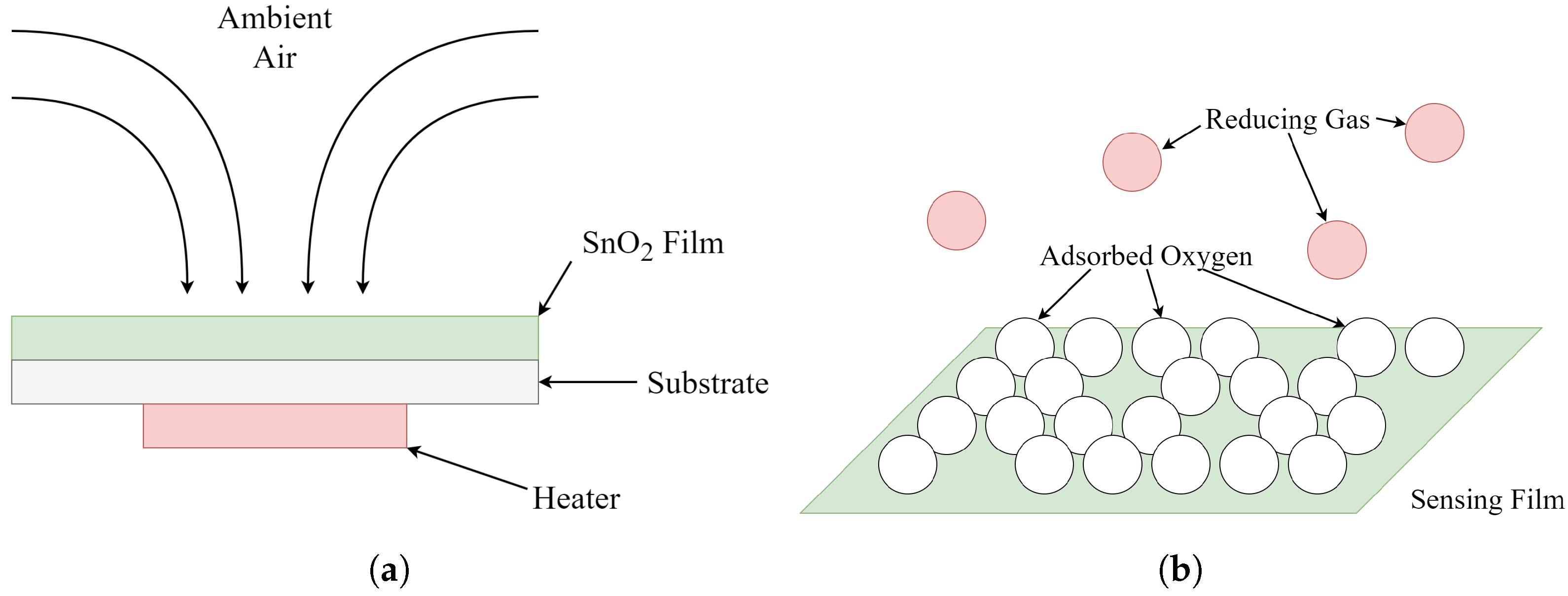
Table 1. These low-cost sensors, most notably the first two sensors manufactured by Figaro USA (Rolling Meadows, IL, USA), are used in many E-Nose devices in existing works. They exhibit some cross-sensitivity, which is noted in
Table 1. However, since their response characteristics are different, we include both sensors for consideration in this work.
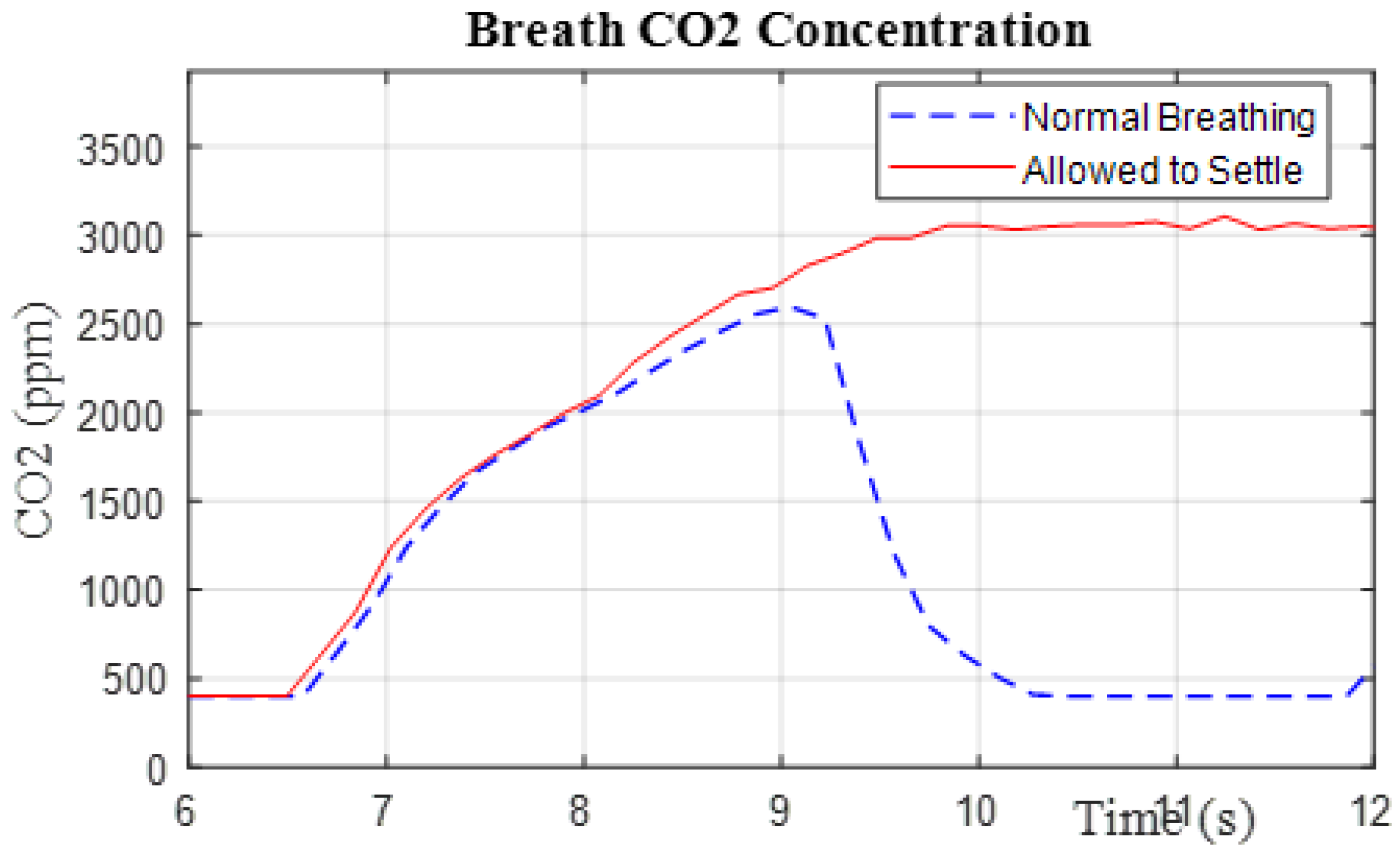
It should be noted that the third sensor is an electrochemical sensor rather than a MOS sensor. We included this sensor to test the applicability of our methodology to other types of gas sensors as well. While the SGX-4OX sensor does have a faster response time than MOS-based sensors, the settling time of the sensor still exceeded 10 s during our observations. While it might be possible for a healthy individual to exhale for this long to obtain a reading, it could present challenges for individuals with COPD or other lung complications. Therefore, we also examine our forecasting methodology on this sensor. All of the sensors used in the system were sourced from Digikey Electronics.
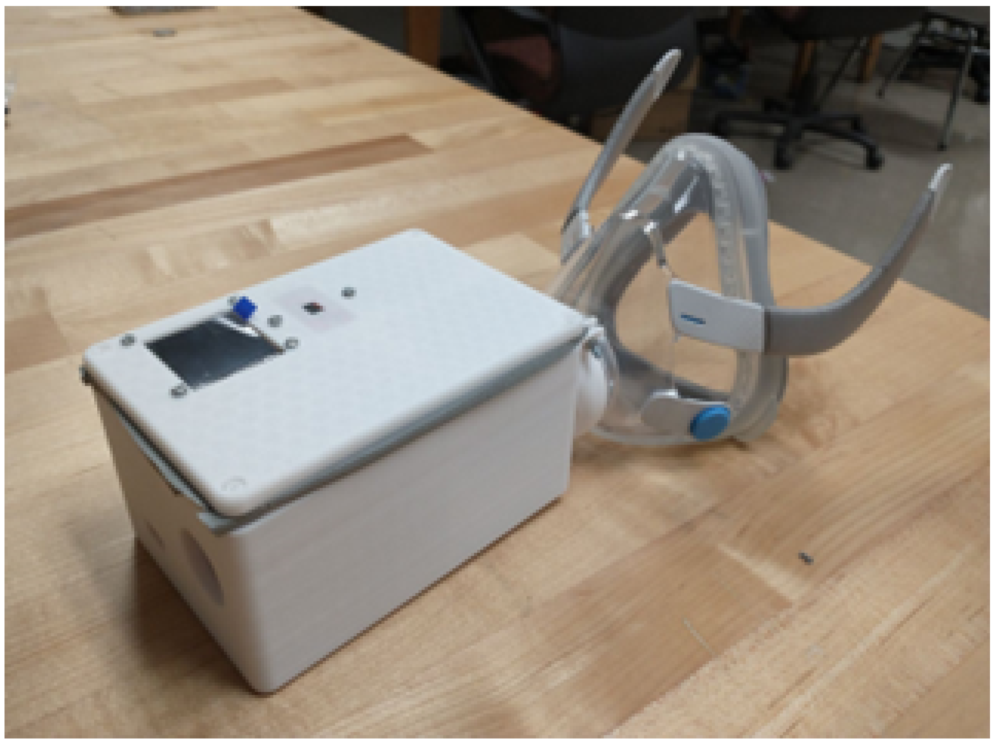
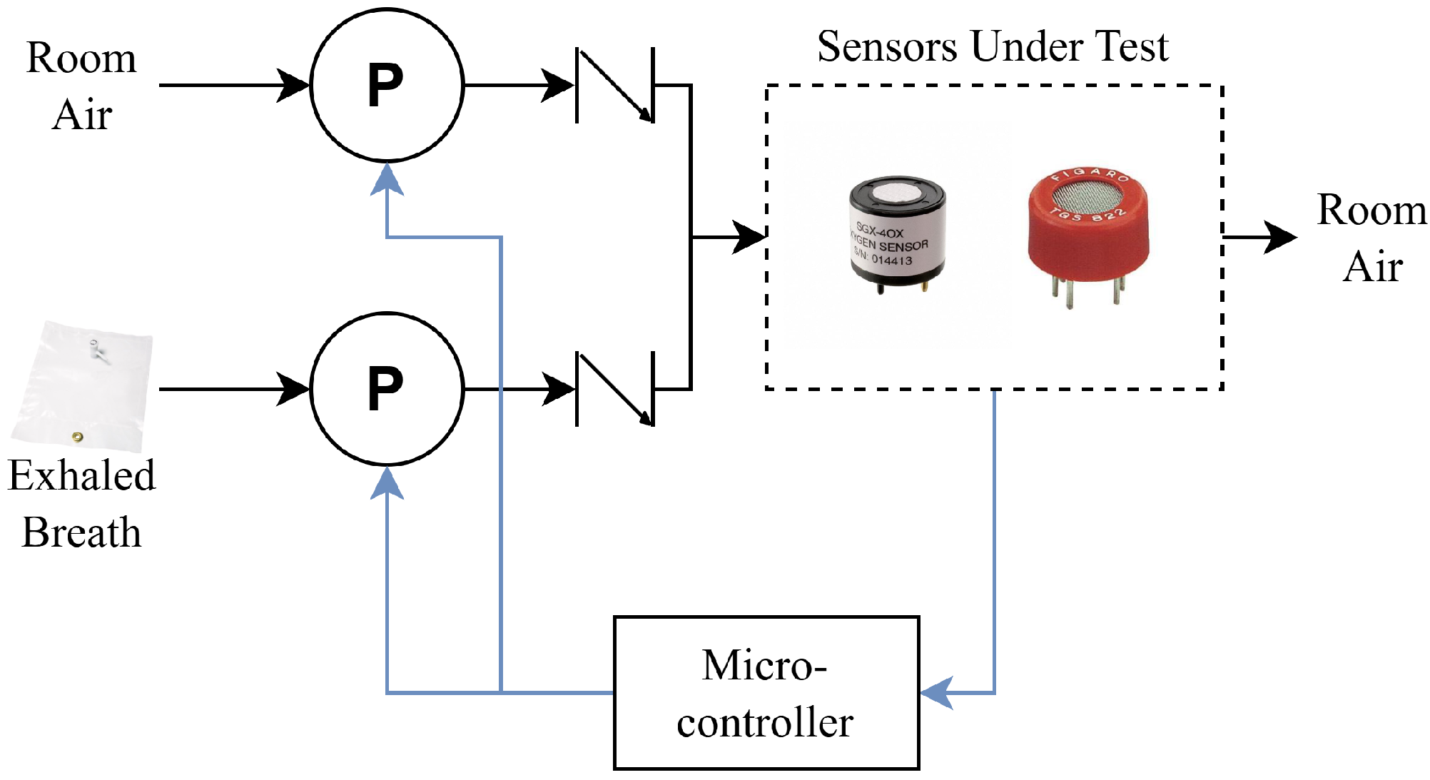
A block diagram of the experimental E-Nose test setup used in this paper is shown in
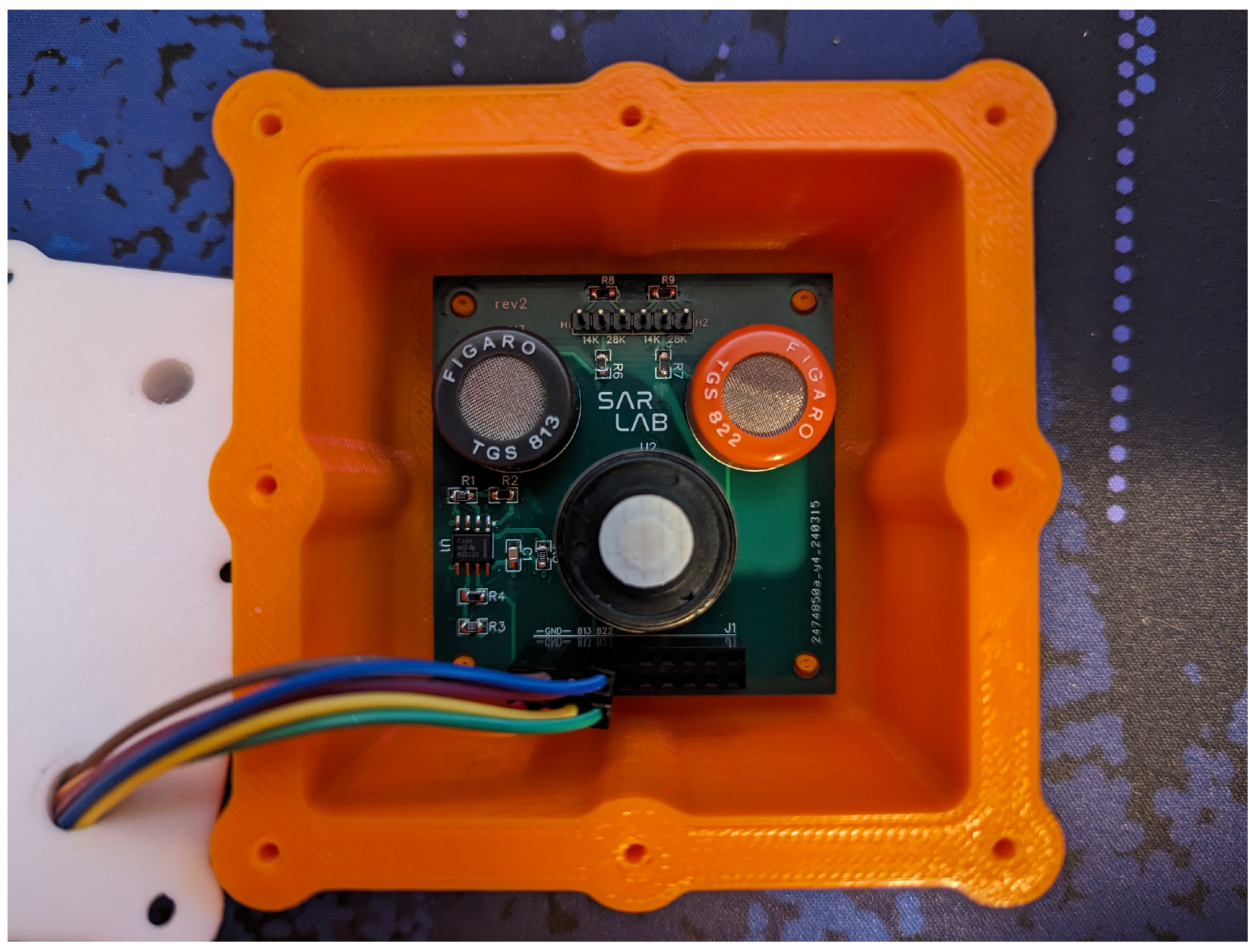
Figure 5, where the arrows signify airflow. The sensors are shown inside their enclosure in
Figure 6. The system utilizes two vacuum pumps that can pump either fresh air from the ambient environment, or exhaled breath samples that are collected in a sampling bag prior to testing. The system is capable of simulating a human breathing cycle by alternating the flow of external air and the exhaled breath sample, though in this paper, we let the sensors fully settle to their steady-state response in order to validate our forecasting methodology.
The resistance of the TGS 822 and TGS 813 sensors were recorded using a simple voltage divider circuit with the output connected to a 12-bit ADC. Both sensors were operated at the manufacturer-specified power rating for the microheater: 660 for the TGS 822, and 835 for the TGS 813. Both sensors underwent an initial burn-in time of continuous power-on for 7 days before being used, and a warm-up period of at least 10 min thereafter before each data collection run. The SGX-4OX, unlike the other two sensors, is an electrochemical sensor that outputs a small current of approximately 90 at 21% oxygen concentration (typical ambient air). This current was measured across a 100 precision shunt with a 2-stage amplifier circuit to boost the signal by a gain of 225. All three sensors were sampled at a rate of 20 during each experiment, though a lower sampling frequency could be used due to the comparatively slow response speed of the gas sensors.
Exhaled breath samples were collected in 10 L foil sampling bags prior to testing. The first step of the experimental procedure involved connecting the sampling bag to the E-Nose, where a vacuum pump was used to pump the contents of the sampling bag through the sensing chamber for 90 s, exposing the sensors to the exhaled breath sample (henceforth, the exposure period). After the exposure period, the sensors undergo a recovery period lasting for 4 min, where ambient room air is pumped through the sensing chamber. This ensures the system is purged of any trace gases from the exposure period, and that the gas sensors have ample time to return to their initial steady-state before the next experiment. This procedure was repeated 25 times by collecting data from one of the authors. For this paper, the system was tested at room temperature, and did not consider the effects of varying humidity or sensitivity of the sensors to different gas mixtures. We plan to address these in a follow-up work; we discuss this in more detail in
Section 5.
After data collection, MATLAB R2025a was used to pre-process the data by converting the ADC values to engineering units. A median filter with a window size of 3 was also applied to suppress external transient noise and erroneous readings from each of the sensor responses. Since a temporal window spanning 3 samples (approximately 100 ) is significantly lower than the response speed of the sensors used in the experiment, a window size of 3 preserves the integrity of the data as much as possible, while removing these erroneous sensor readings.
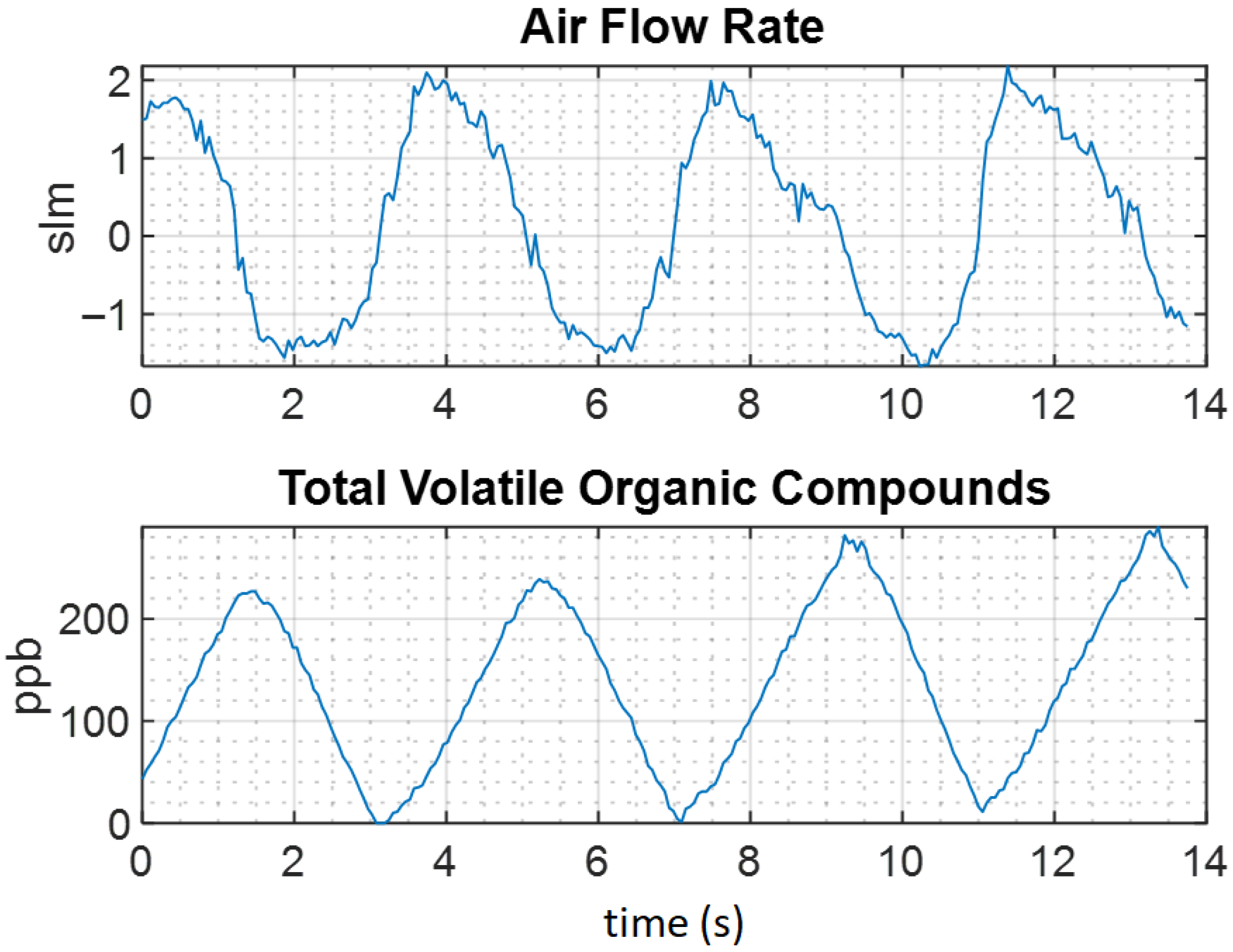
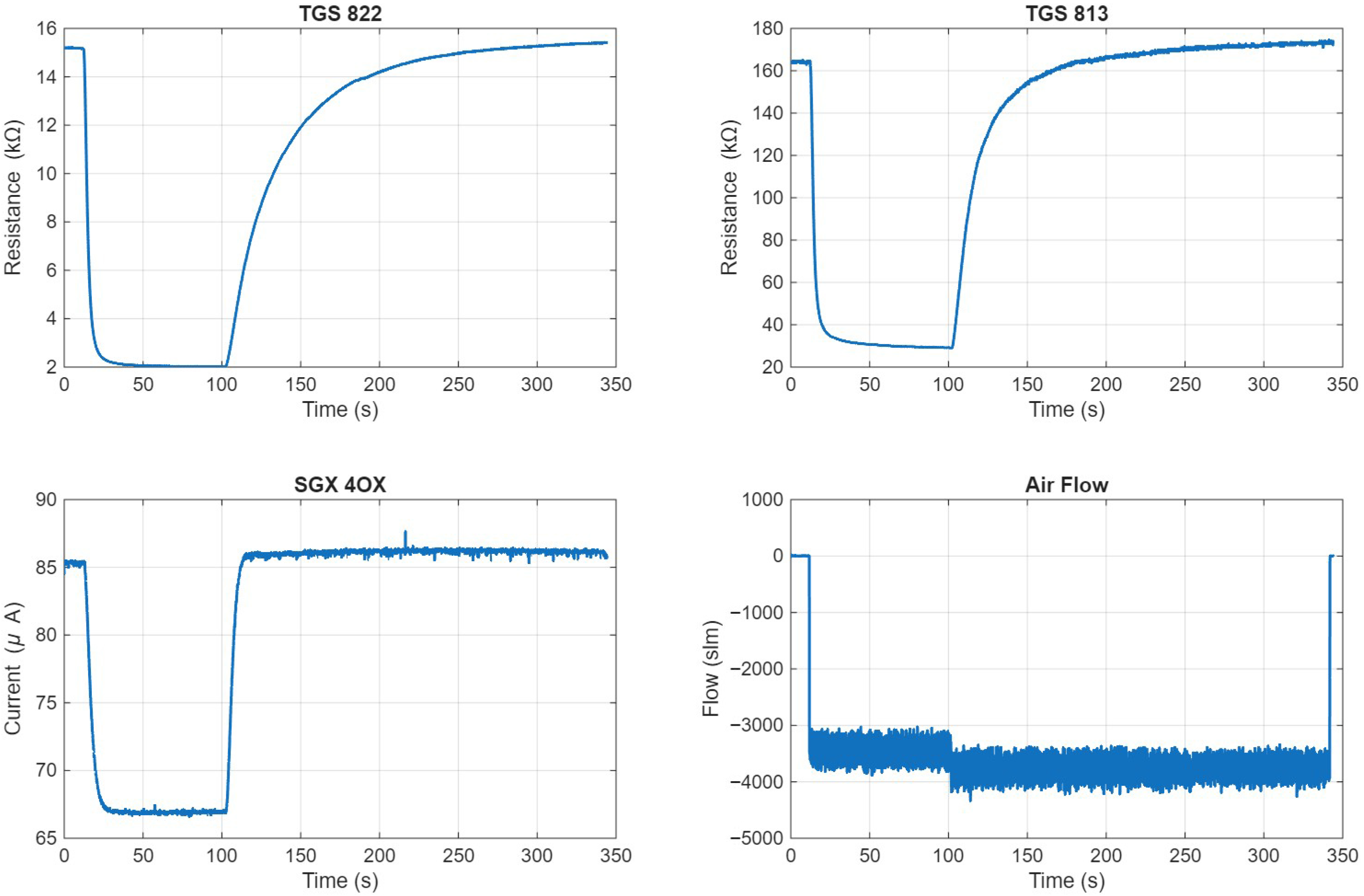
Figure 7 shows a sample of pre-processed data collected from the testing apparatus. A Sensirion SFM3200 airflow sensor was also included to measure the airflow through the sensing enclosure, which was used to determine the beginning of the exposure period. This was done by finding the time
where the airflow exceeds
slm, indicating that the vacuum pump is enabled. The sensor response for the three gas sensors between
and
was then extracted. This yielded 25 samples of pre-processed data, each containing three sensor responses 85 s long.
3.2. Data Analysis & Model Fitting
MATLAB’s Curve Fitting Toolbox was used to find and fit an appropriate model to the collected gas sensor data. The fit was conducted using the nonlinear least squares (NLLSQ) method, and goodness-of-fit was evaluated using the root mean squared error (RMSE) between the ground-truth and model prediction across all sample points on the curve.
Four different mathematical models were evaluated based on the modeling assumptions outlined in
Section 2. These are summarized in
Table 2, where the average RMSE and normalized RMSE (normalized to the range of the signal) for each model across all sensor responses is shown. It should be noted that the fit to each sensor is shown separately, as the difference in response characteristics of the sensors makes a direct comparison meaningless.
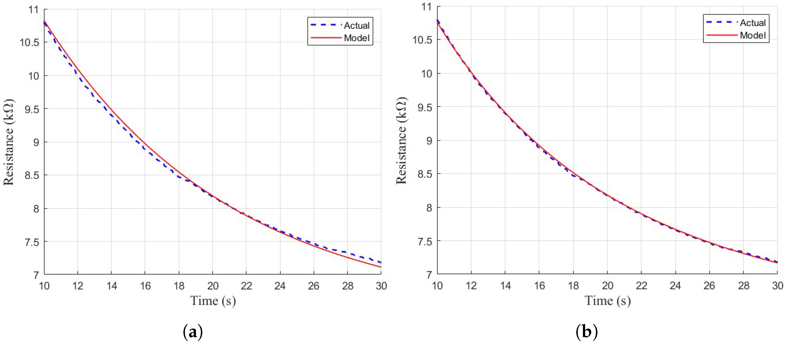
Two first-order exponential models of the forms
and
were fit first, as these most closely resemble the Langmuir dynamics we expected to observe. Although these two models characterize the general shape of the response well, they fail to model the initial transient behavior of the sensor due to their first-order nature. Both of these first-order models performed very similarly in most scenarios, as the NLLSQ solver found a solution where
for many of the breath samples, indicating that model 2 tends to degenerate towards model 1. This is reflected in the small difference in performance between models 1 and 2 in
Table 2. The fit of both models 1 and 2 can be seen from a qualitative perspective in
Figure 8.
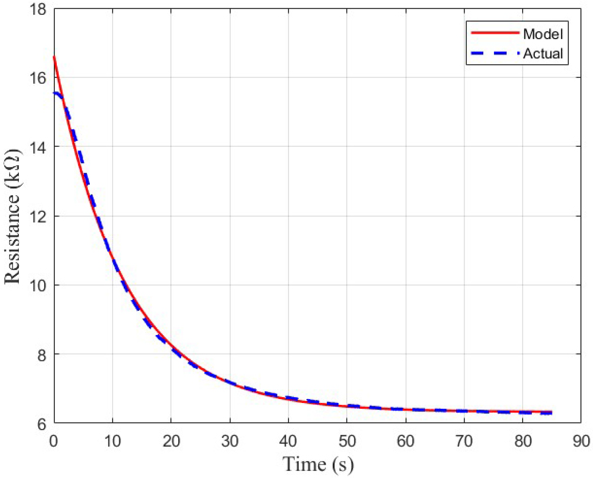
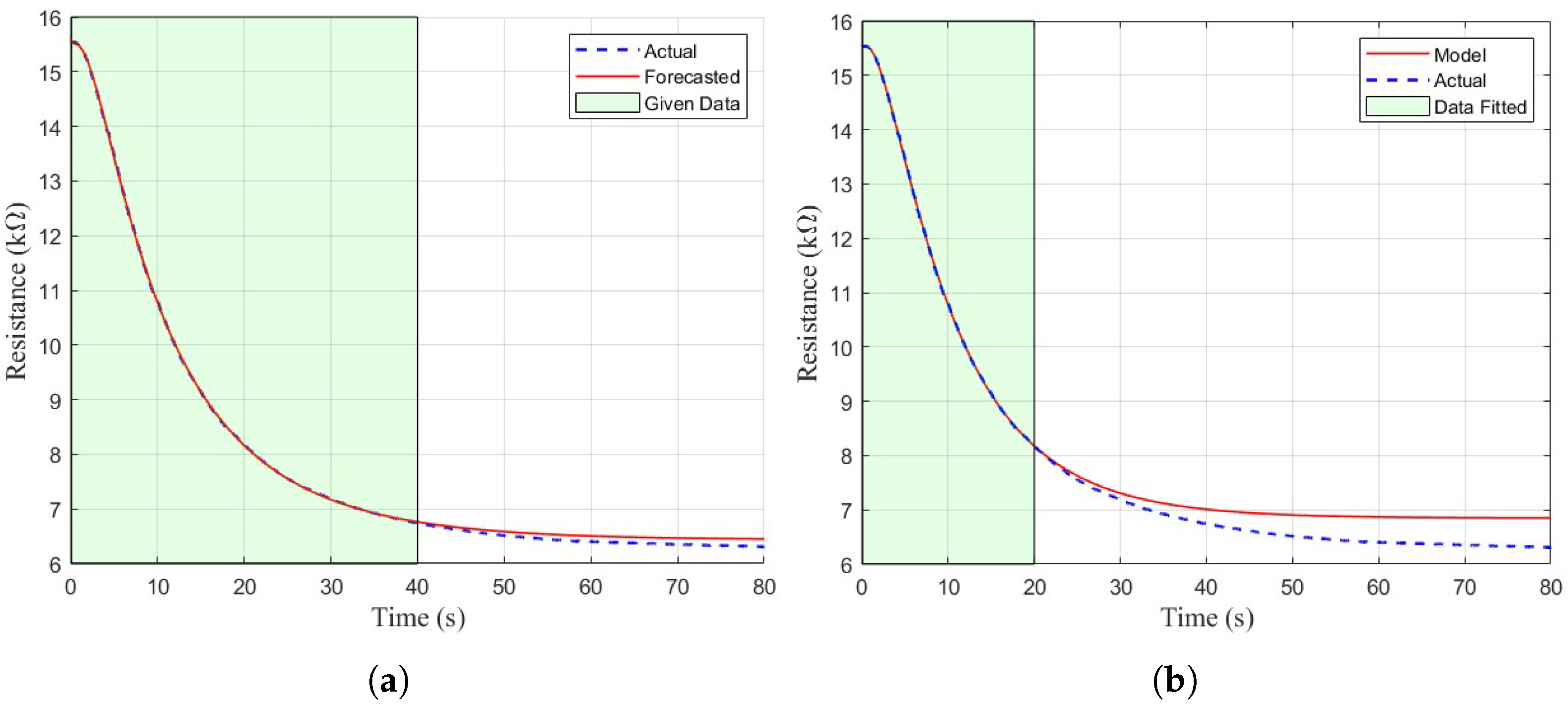
We believe that the initial transient observed in the sensor response is due to second-order dynamics caused by the initial diffusion of gas into the sensing chamber. Thus, to improve the goodness-of-fit, two second-order models were considered. The first is a simple second-order exponential in the form of , and the second model is a sum of one exponential function and a stretched exponential function, in the form of .
The two second-order models exhibited a much better fit to the sensor data. Although the simple second-order model mostly fits the shape of the curve, there is some non-exponentiality to the sensor response where the model deviates slightly from the actual response, as shown in
Figure 9. The stretched exponential function is better able to model these non-exponential characteristics, where the simple model slightly overshoots or undershoots in some areas compared to the ground-truth.
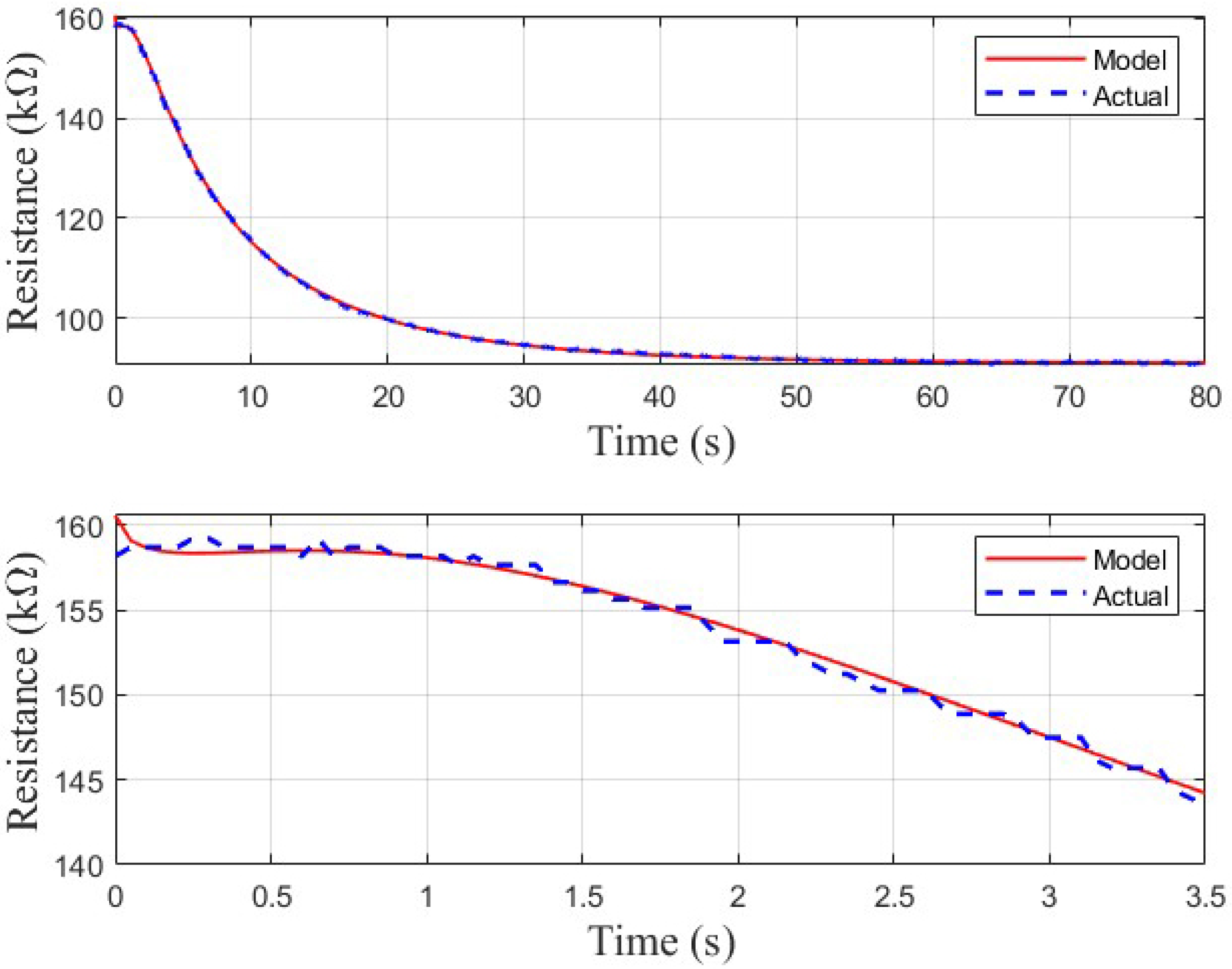
The second-order model including the stretched exponential is overall a much better fit, as shown in
Figure 10. Aside from a slight transient at the beginning of the curve, the model fits the ground-truth sensor response significantly better than the simple second-order model. This is verified by
Table 2, which indicates that the second-order stretched exponential model exhibits a lower RMSE on average than the simple second-order model for all sensors.
Aside from the models shown in
Table 2, higher-order models of the general form shown in Equation (
7) were also examined, with
n being the order of the model. Third-order models and higher did not demonstrate improved performance compared to second-order models due to over-parameterization. Fitted models commonly contained two or more confounding exponential terms with wide confidence intervals, indicating that those terms are redundant and can freely change oppositely to each other with little impact on the resulting model.
Lastly, the addition of a delay term
d was also investigated, as shown in Equation (
8). Similarly to the higher-order models that were examined, the addition of a delay to each exponential term also resulted in over-parameterization, which made convergence of the NLLSQ algorithm more difficult to achieve.
Thus, the final model we selected was the summation of a stretched exponential term and one additional standard exponential, shown by Equation (
9) (Model 4 from
Table 2). We found that this model most consistently models the behavior of each gas sensor in our testing apparatus.