Author Contributions
Conceptualization, J.L.; Methodology, L.X.; Software, L.X.; Formal analysis, Y.L.; Investigation, X.Z. and J.L.; Resources, X.Z., J.L. and L.X.; Data curation, Y.L. and L.X.; Writing—original draft, Y.L.; Writing—review & editing, X.Z., Y.L. and Y.Y.; Visualization, Y.Y.; Supervision, X.Z., Y.Y. and J.L.; Funding acquisition, Y.Y. All authors have read and agreed to the published version of the manuscript.
Figure 1.
Original finger vein image.
Figure 1.
Original finger vein image.
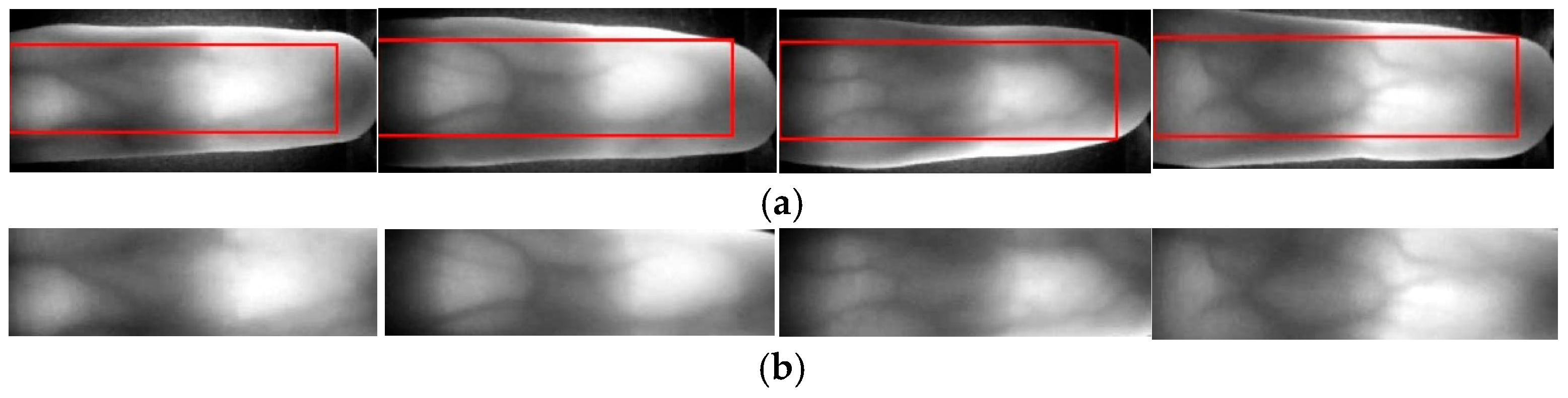
Figure 2.
ROI localization results for four finger vein samples acquired under different lighting and vein patterns: (a) ROI annotation showing the automatically detected regions of interest; (b) final extracted ROI regions after cropping corresponding to the annotated areas.
Figure 2.
ROI localization results for four finger vein samples acquired under different lighting and vein patterns: (a) ROI annotation showing the automatically detected regions of interest; (b) final extracted ROI regions after cropping corresponding to the annotated areas.
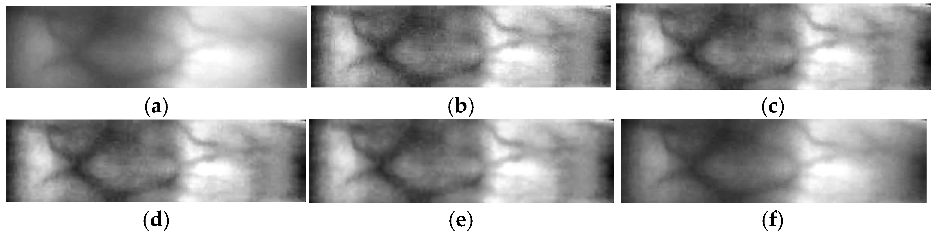
Figure 3.
Illustration of the finger vein image enhancement and denoising process. Step-by-step results of the enhancement and denoising process: (a) original ROI; (b) contrast enhancement using CLAHE; (c) after median filtering; (d) after Gaussian filtering; (e) after wavelet-based denoising with soft thresholding; (f) final enhanced result after linear fusion.
Figure 3.
Illustration of the finger vein image enhancement and denoising process. Step-by-step results of the enhancement and denoising process: (a) original ROI; (b) contrast enhancement using CLAHE; (c) after median filtering; (d) after Gaussian filtering; (e) after wavelet-based denoising with soft thresholding; (f) final enhanced result after linear fusion.
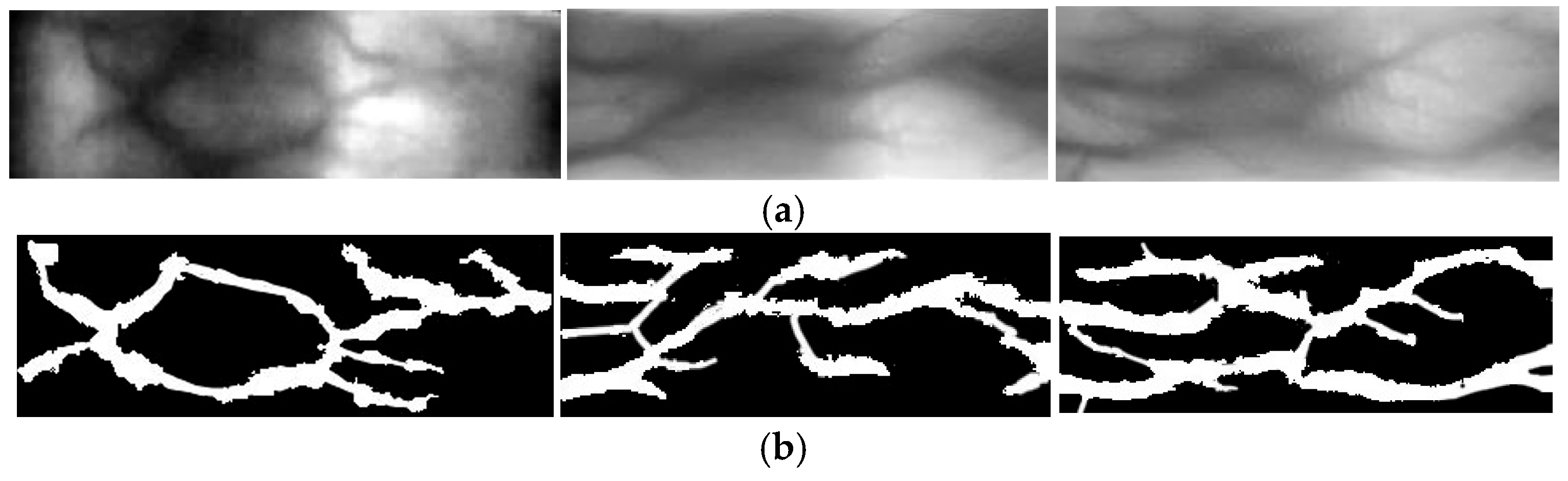
Figure 4.
Binarization results before and after processing for three different finger vein samples: (a) before processing; (b) after processing.
Figure 4.
Binarization results before and after processing for three different finger vein samples: (a) before processing; (b) after processing.
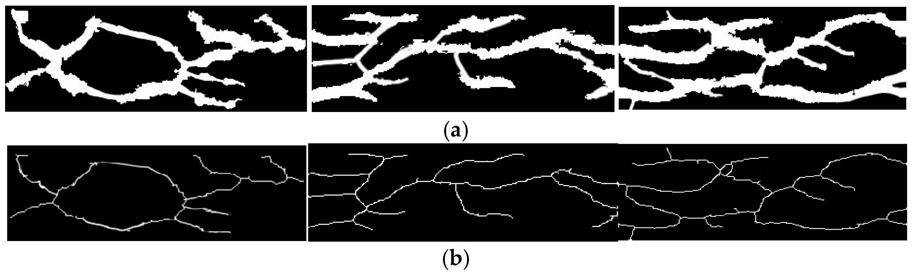
Figure 5.
Vein skeletonization results before and after processing for multiple finger vein samples: (a) before processing (binarized images); (b) after skeletonization.
Figure 5.
Vein skeletonization results before and after processing for multiple finger vein samples: (a) before processing (binarized images); (b) after skeletonization.
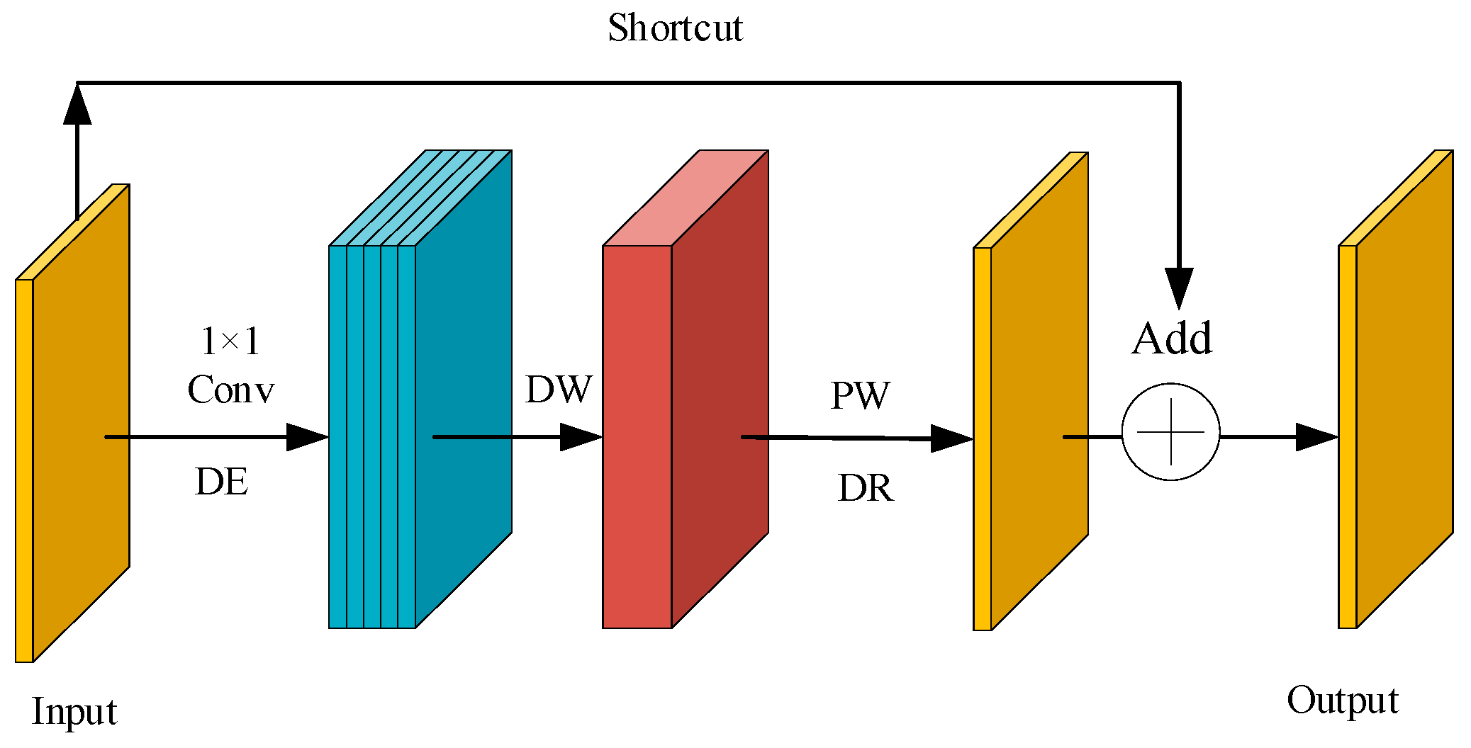
Figure 6.
Linear bottleneck inverted residual structure.
Figure 6.
Linear bottleneck inverted residual structure.
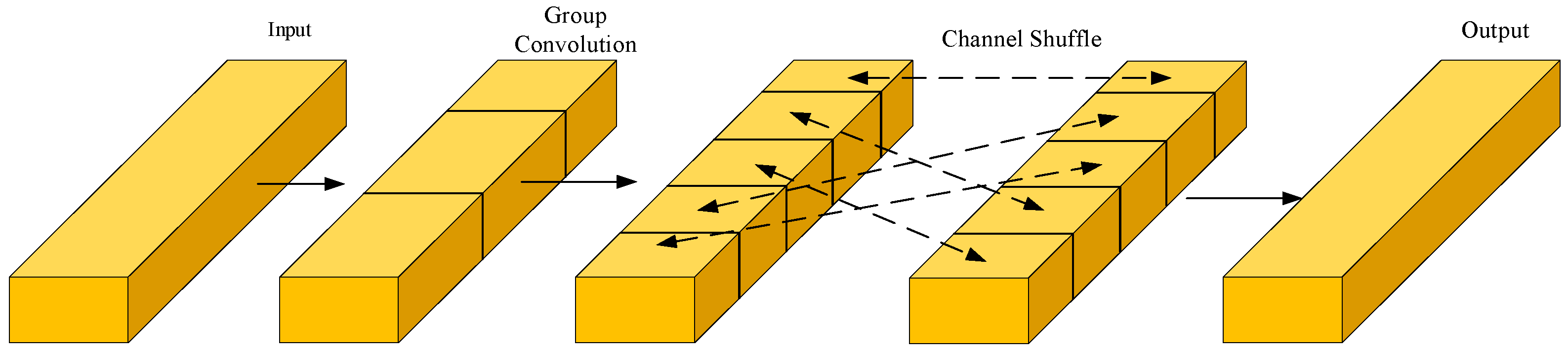
Figure 7.
Channel shuffle operation in ShuffleNet.
Figure 7.
Channel shuffle operation in ShuffleNet.
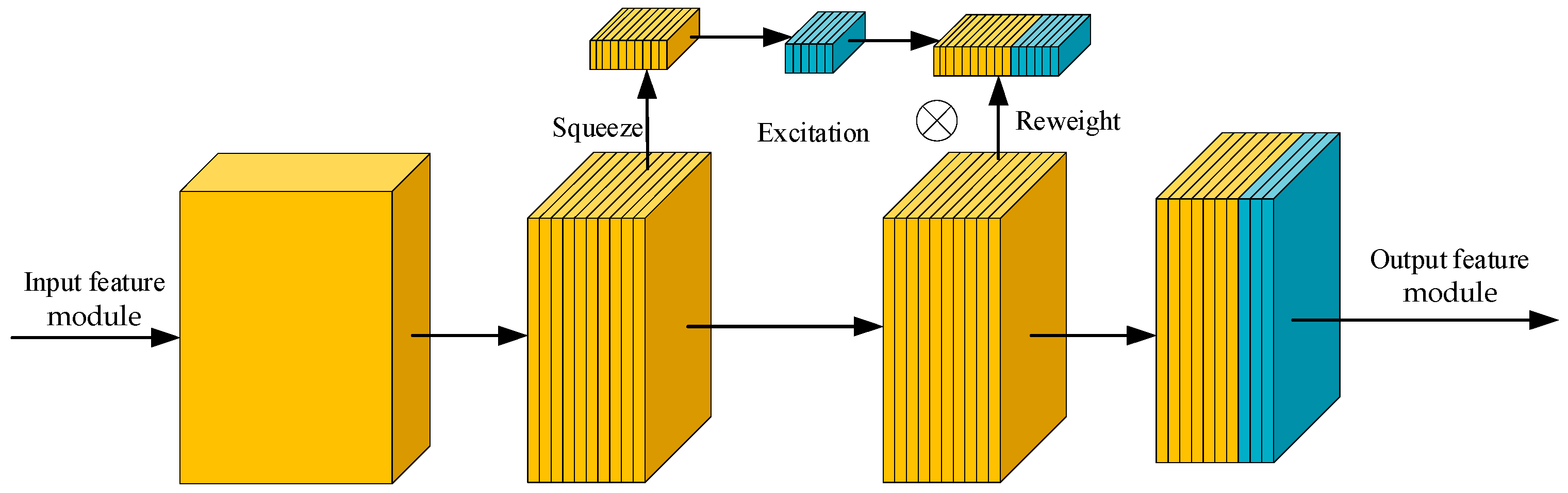
Figure 8.
SE Channel attention module.
Figure 8.
SE Channel attention module.
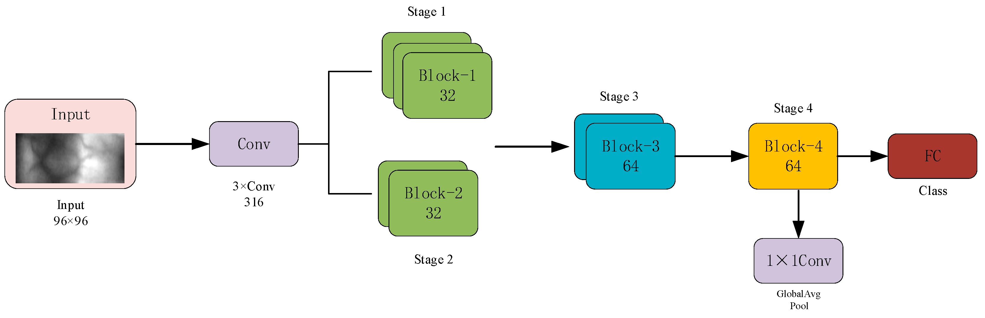
Figure 9.
Overall architecture of the proposed LCNN.
Figure 9.
Overall architecture of the proposed LCNN.
Figure 10.
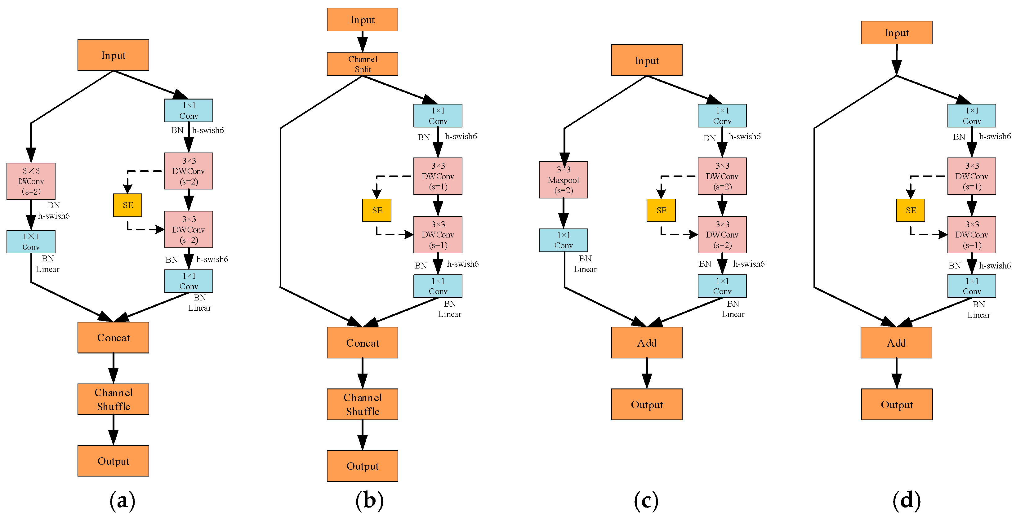
Structures of the Four Lightweight Convolutional Blocks in the Proposed LCNN. (a) block-1; (b) block-2; (c) block-3; (d) block-4.
Figure 10.
Structures of the Four Lightweight Convolutional Blocks in the Proposed LCNN. (a) block-1; (b) block-2; (c) block-3; (d) block-4.
Figure 11.
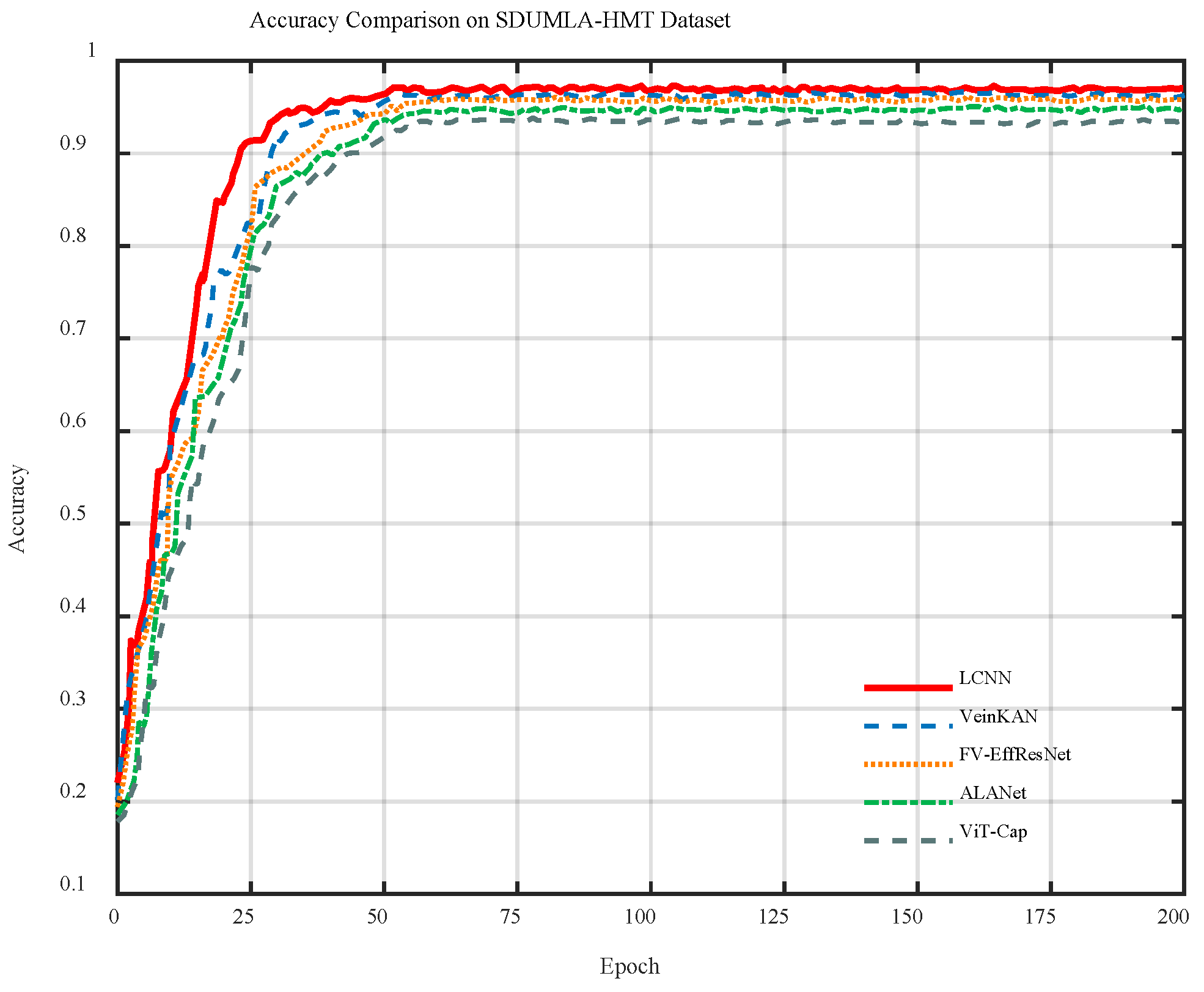
Accuracy curves of different models on the SDUMLA-HMT dataset.
Figure 11.
Accuracy curves of different models on the SDUMLA-HMT dataset.
Figure 12.
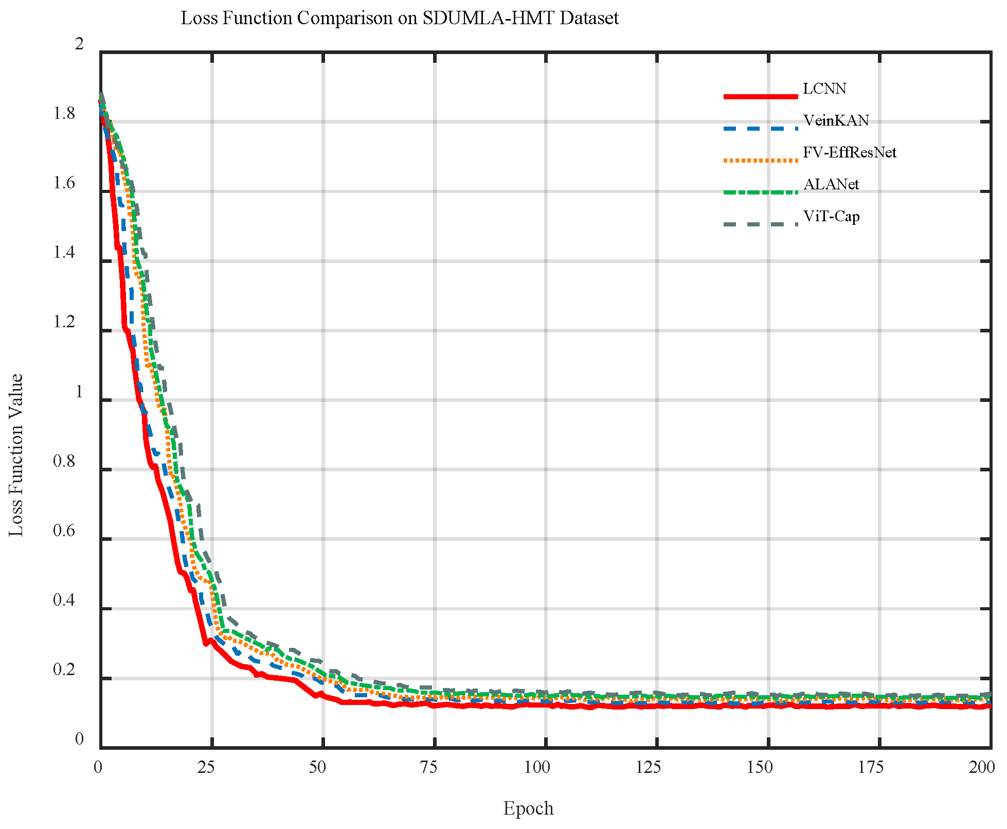
Loss curves of different models on the SDUMLA-HMT dataset.
Figure 12.
Loss curves of different models on the SDUMLA-HMT dataset.
Figure 13.
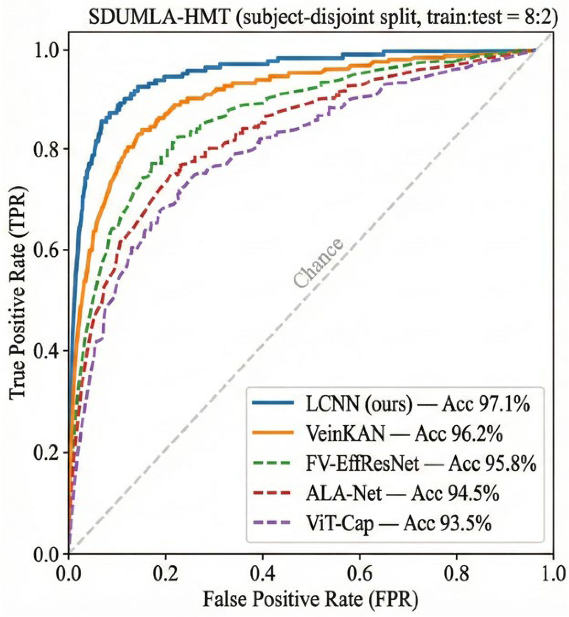
ROC curves of the SDUMLA-HMT finger vein dataset.
Figure 13.
ROC curves of the SDUMLA-HMT finger vein dataset.
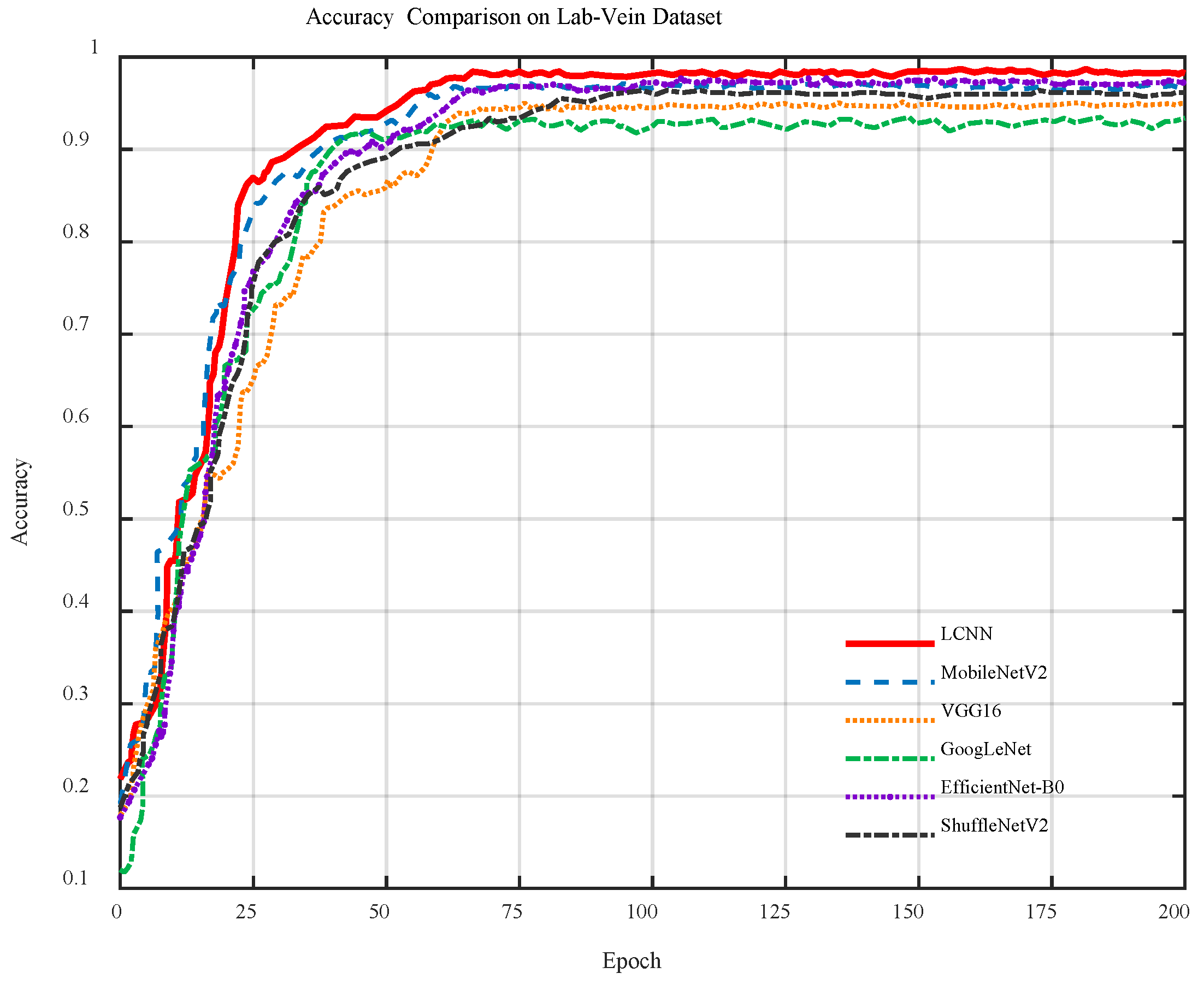
Figure 14.
Accuracy curves of different models on the Lab-Vein dataset.
Figure 14.
Accuracy curves of different models on the Lab-Vein dataset.
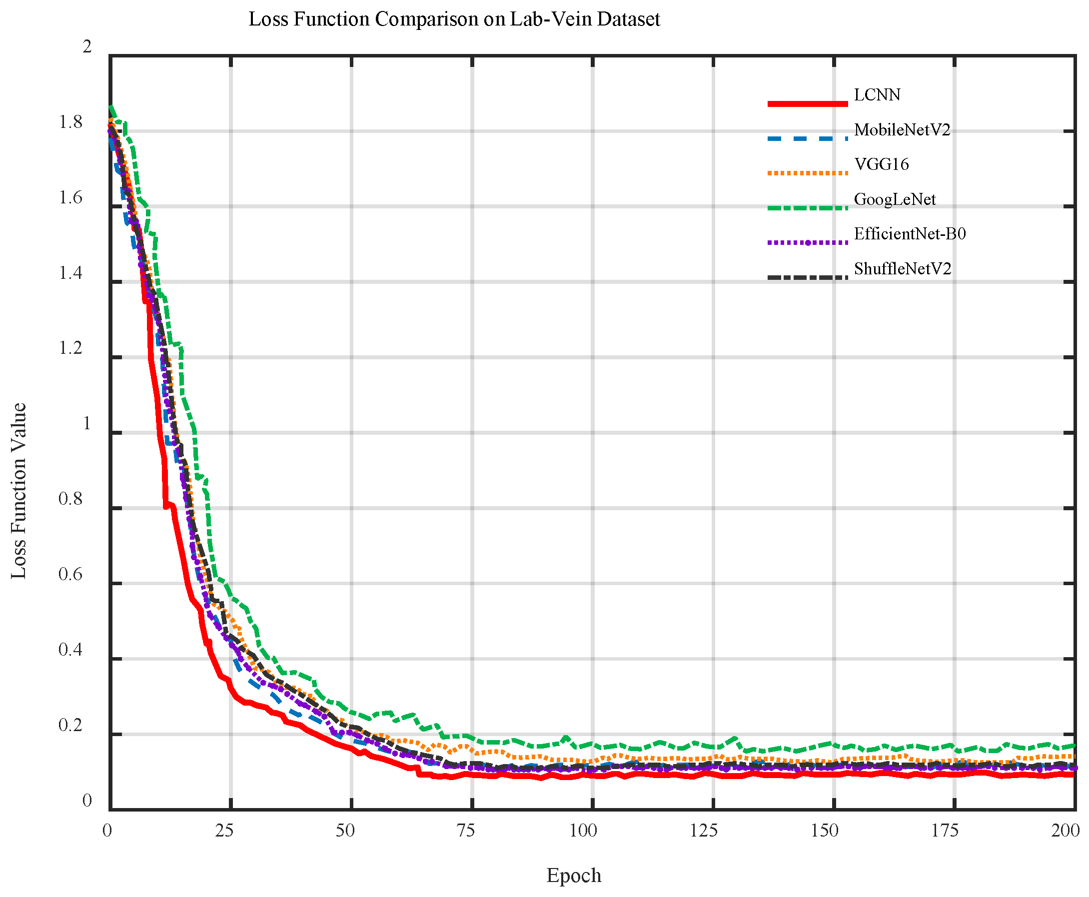
Figure 15.
Loss curves of different models on the Lab-Vein dataset.
Figure 15.
Loss curves of different models on the Lab-Vein dataset.
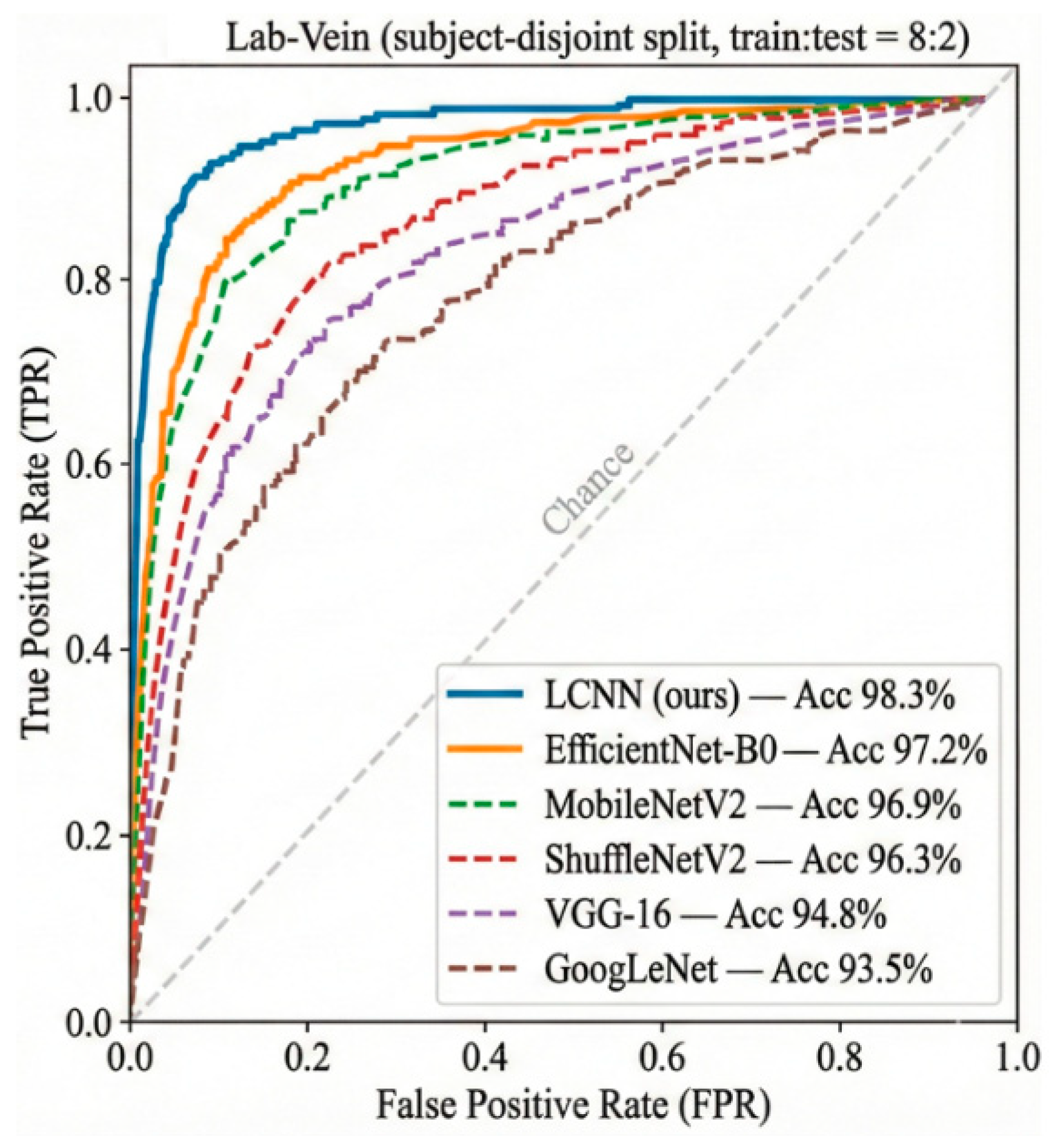
Figure 16.
ROC curves of the Lab-Vein finger vein dataset.
Figure 16.
ROC curves of the Lab-Vein finger vein dataset.
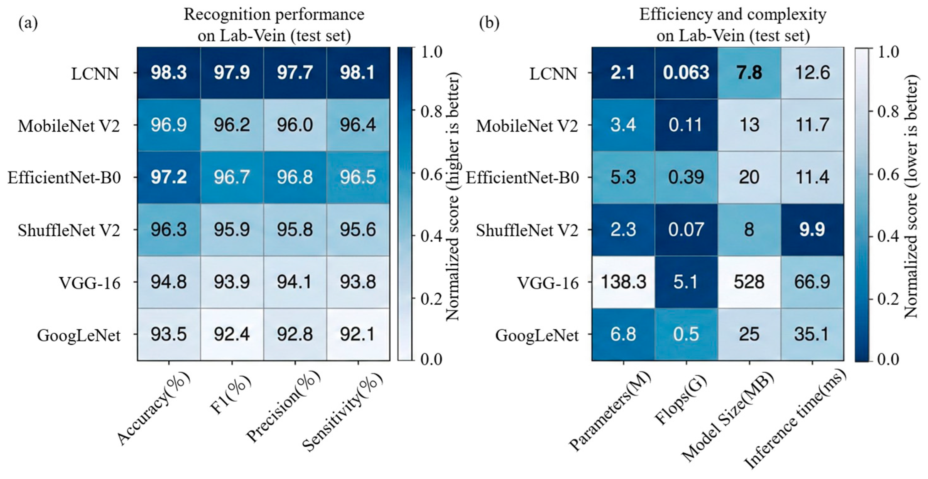
Figure 17.
Heatmap comparison of recognition performance and deployment efficiency on the Lab-Vein test set. (a) Recognition effectiveness in terms of Accuracy, F1-score, Precision, and Sensitivity (darker shades = higher column-wise normalized scores). (b) Efficiency and complexity comparison including Parameters, FLOPs, Model Size, and Inference Time (darker shades = lower computational cost).
Figure 17.
Heatmap comparison of recognition performance and deployment efficiency on the Lab-Vein test set. (a) Recognition effectiveness in terms of Accuracy, F1-score, Precision, and Sensitivity (darker shades = higher column-wise normalized scores). (b) Efficiency and complexity comparison including Parameters, FLOPs, Model Size, and Inference Time (darker shades = lower computational cost).
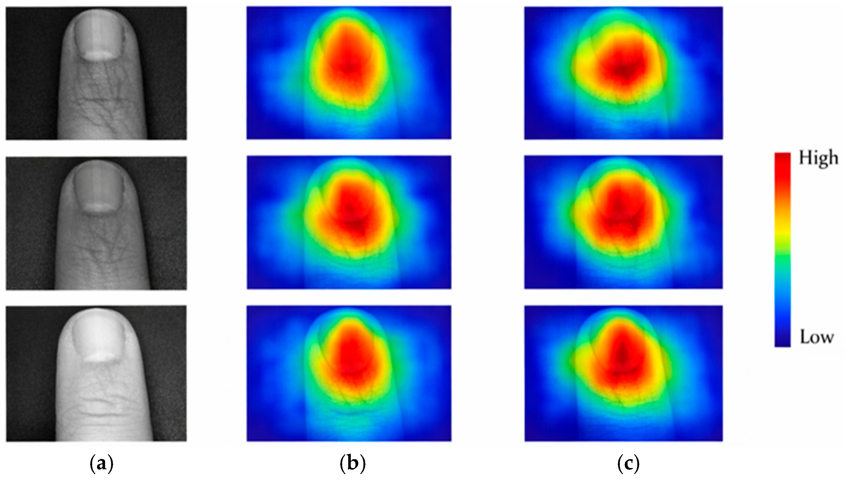
Figure 18.
Grad-CAM attention heatmaps for finger-vein recognition models. (a) Input images, (b) EfficientNet-B0 heatmaps, (c) LCNN heatmaps. The proposed LCNN focuses mainly on the central vascular regions, confirming its better feature localization ability.
Figure 18.
Grad-CAM attention heatmaps for finger-vein recognition models. (a) Input images, (b) EfficientNet-B0 heatmaps, (c) LCNN heatmaps. The proposed LCNN focuses mainly on the central vascular regions, confirming its better feature localization ability.
Table 1.
Performance comparison between classical and DL-based segmentation methods.
Table 1.
Performance comparison between classical and DL-based segmentation methods.
| Method | Dice (%) | IoU (%) | Inference Time (ms) | Parameters (M) |
|---|
| Otsu-Based (Proposed) | 90.5 | 82.8 | 8.5 | - |
| U-Net | 91.8 | 84.4 | 37.2 | 7.9 |
| MobileNet-U-Net | 90.9 | 83.7 | 18.6 | 1.5 |
Table 2.
Structural configuration of the proposed LCNN.
Table 2.
Structural configuration of the proposed LCNN.
| Layer | Input Size | Operator/Block | Output Channels | Stride |
|---|
| Input | 96 × 96 × 1 | - | - | - |
| Conv | 96 × 96 × 1 | 3 × 3 Conv | 8 | 2 |
| MaxPool | 48 × 48 × 8 | 3 × 3 MaxPool | 8 | 2 |
| Stage1 | 12 × 12 × 16 | block-1 × 1 | 16 | 2 |
| Stage2 | 12 × 12 × 16 | block-2 × 2 | 32 | 1 |
| Stage3 | 12 × 12 × 32 | block-3 × 2 | 64 | 1 |
| Stage4 | 12 × 12 × 64 | block-4 × 1 | 64 | 1 |
| Conv1 × 1 | 12 × 12 × 64 | 1 × 1 Conv | 128 | 1 |
| GAP | 1 × 1×128 | Global AvgPool | 128 | - |
| FC | 1 × 1×128 | Fully connected layer | N | - |
Table 3.
System Configuration of the Experimental Environment.
Table 3.
System Configuration of the Experimental Environment.
| Environment Configuration | Model Version |
|---|
| CPU processor | Intel Core i7-14650HX @ 2.20 GHz |
| Internal memory | 32GB |
| GPU graphics card | NVIDIA GeForce RTX 4060 |
| CUDA version | 11.1 |
| CUDNN version | 8.1 |
| Python version | 3.8 |
| PyTorch version | 2.2.1 |
| Operating system | Windows 11 |
Table 4.
Performance comparison of different models on the SDUMLA-HMT dataset.
Table 4.
Performance comparison of different models on the SDUMLA-HMT dataset.
| Model Name | Years | Accuracy/% | EER (%) | Parameters (M) | Time (ms) |
|---|
| LCNN (Ours) | 2026 | 97.1 | 0.81 | 2.1 | 3.6 |
| ViT-Cap [12] | 2022 | 93.5 | 4.13 | - | - |
| ALANet [13] | 2023 | 94.5 | 0.53 | 2.55 | 4.32 |
| FV-EffResNet [15] | 2024 | 95.8 | 0.43 | 1.32 | 5.60 |
| VeinKAN [16] | 2025 | 96.2 | - | 34.81 | 1.0096 |
Table 5.
Performance comparison of different models on the Lab-Vein dataset.
Table 5.
Performance comparison of different models on the Lab-Vein dataset.
| Model Name | Accuracy (%) | EER (%) | F1 (%) | Precision (%) | Sensitivity (%) |
|---|
| LCNN(ours) | 98.3 | 0.32 | 97.9 | 97.7 | 98.1 |
| MobileNet V2 | 96.9 | 0.68 | 96.2 | 96.0 | 96.4 |
| EfficientNet-B0 | 97.2 | 0.55 | 96.7 | 96.8 | 96.5 |
| ShuffleNet V2 | 96.3 | 0.92 | 95.9 | 95.8 | 95.6 |
| VGG-16 | 94.8 | 1.664 | 93.9 | 94.1 | 93.8 |
| GoogLeNet | 93.5 | 2.13 | 92.4 | 92.8 | 92.1 |
Table 6.
Comparison of parameter count, computational cost, and model size across different models.
Table 6.
Comparison of parameter count, computational cost, and model size across different models.
| Model Name | Parameters (M) | FLOPs (G) | Model Size (MB) |
|---|
| LCNN(Ours) | 2.1 | 0.063 | 7.8 |
| MobileNetV2 | 3.4 | 0.11 | 13 |
| EfficientNet-B0 | 5.3 | 0.39 | 20 |
| ShuffleNet V2 | 2.3 | 0.07 | 8 |
| VGG-16 | 138.3 | 5.1 | 528 |
| GoogLeNet | 6.8 | 0.5 | 25 |
Table 7.
Inference speed and relative acceleration of different models.
Table 7.
Inference speed and relative acceleration of different models.
| Model Name | Time (ms) | Relative Speed-Up (×VGG-16) |
|---|
| LCNN (Ours) | 12.6 | 5.31 |
| MobileNetV2 | 11.7 | 5.72 |
| EfficientNet-B0 | 11.4 | 6.52 |
| ShuffleNet V2 | 9.9 | 7.37 |
| VGG-16 | 66.9 | 1.00 |
| GoogLeNet | 35.1 | 1.91 |
Table 8.
Ablation study: recognition performance of different configurations.
Table 8.
Ablation study: recognition performance of different configurations.
| Model Settings | Precision (%) | F1 (%) |
|---|
| Baseline | 97.0 | 96.6 |
| +SE | 97.6 | 97.2 |
| +Shuffle | 97.4 | 97.0 |
| +SE +Shuffle | 98.0 | 97.6 |
| Full (Ours) | 98.3 | 97.9 |
Table 9.
Model complexity comparison of different ablation configurations.
Table 9.
Model complexity comparison of different ablation configurations.
| Model Settings | Parameters (M) | FLOPs (G) | Time (ms) |
|---|
| Baseline | 1.85 | 0.057 | 11.8 |
| +SE | 2.03 | 0.060 | 12.2 |
| +Shuffle | 1.86 | 0.057 | 11.9 |
| +SE + Shuffle | 2.05 | 0.060 | 12.3 |
| Full (Ours) | 2.10 | 0.063 | 12.6 |