A Denoising Algorithm for Maglev Gyro Jump Data Based on Bayesian Ensemble Time-Series Segmentation


Abstract
1. Introduction
- (1)
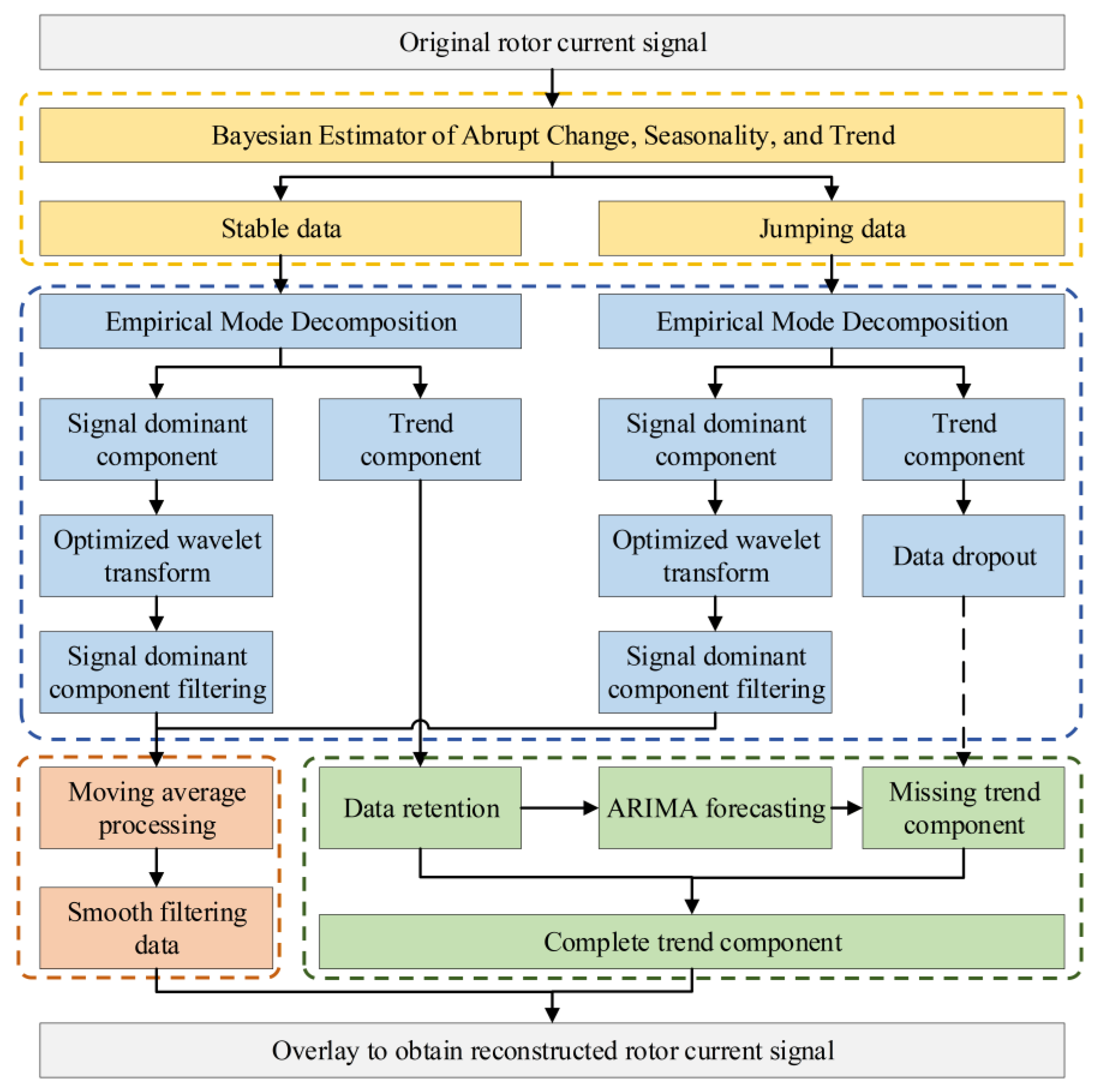
- A BEAST-based probabilistic time-series segmentation strategy is introduced to automatically identify rotor current change points without requiring manually defined segmentation windows, thereby improving the adaptability under varying disturbance conditions.
- (2)
- A segmented adaptive denoising framework is proposed in which stationary and jump intervals are processed independently using EMD-based dominant component extraction and optimized wavelet filtering with different parameter settings. This strategy effectively suppresses noise while preserving the signal continuity.
- (3)
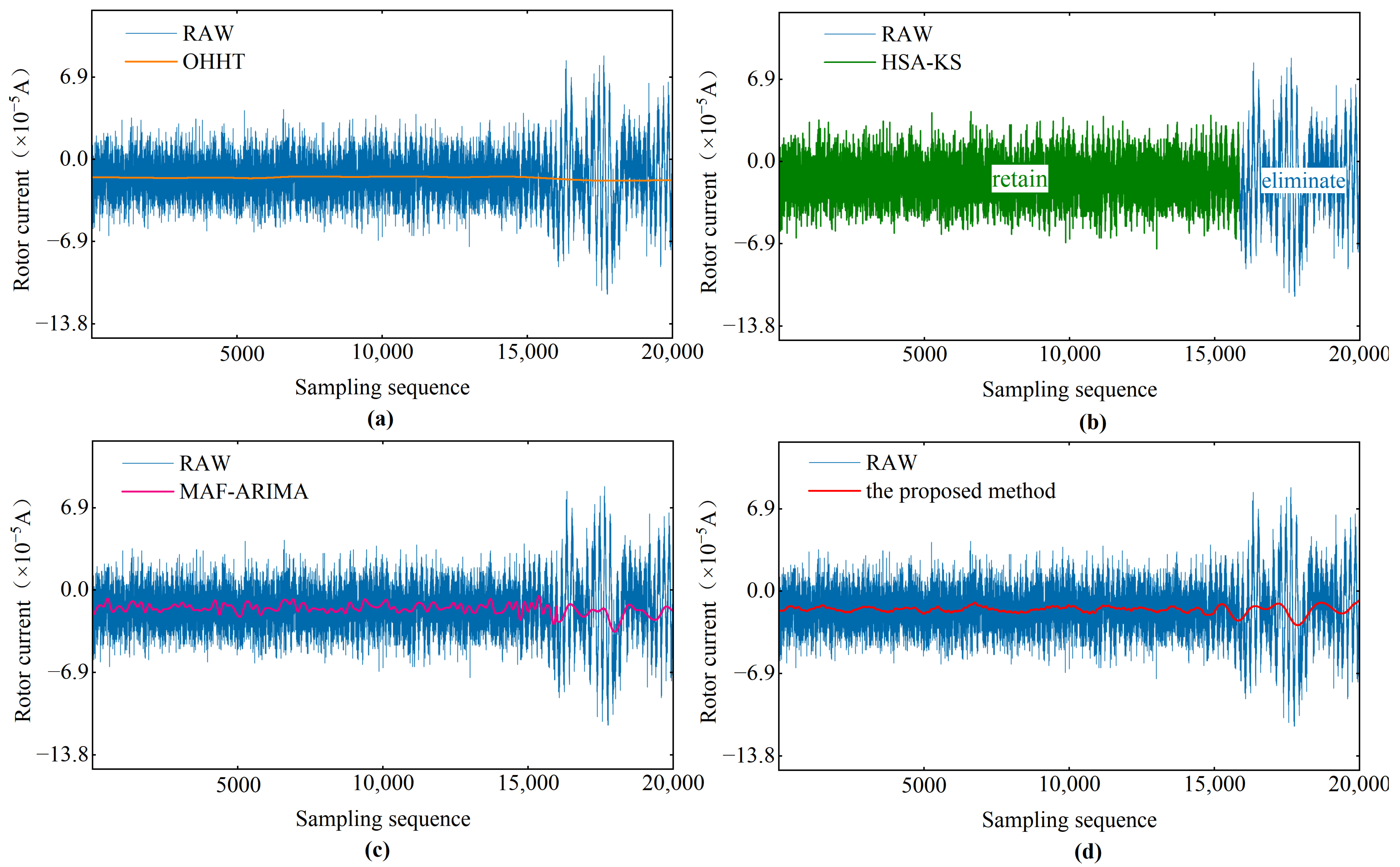
- Comprehensive experiments conducted on 12 groups of field-collected rotor current signals demonstrated that the proposed method achieved a superior denoising performance compared with the OHHT, HSA-KS, and MAF-ARIMA in terms of both the internal and external compliance accuracy, while further improving the adaptability and robustness.
2. Proposed Methodology
2.1. BEAST-Based Time-Series Segmentation
- (1)
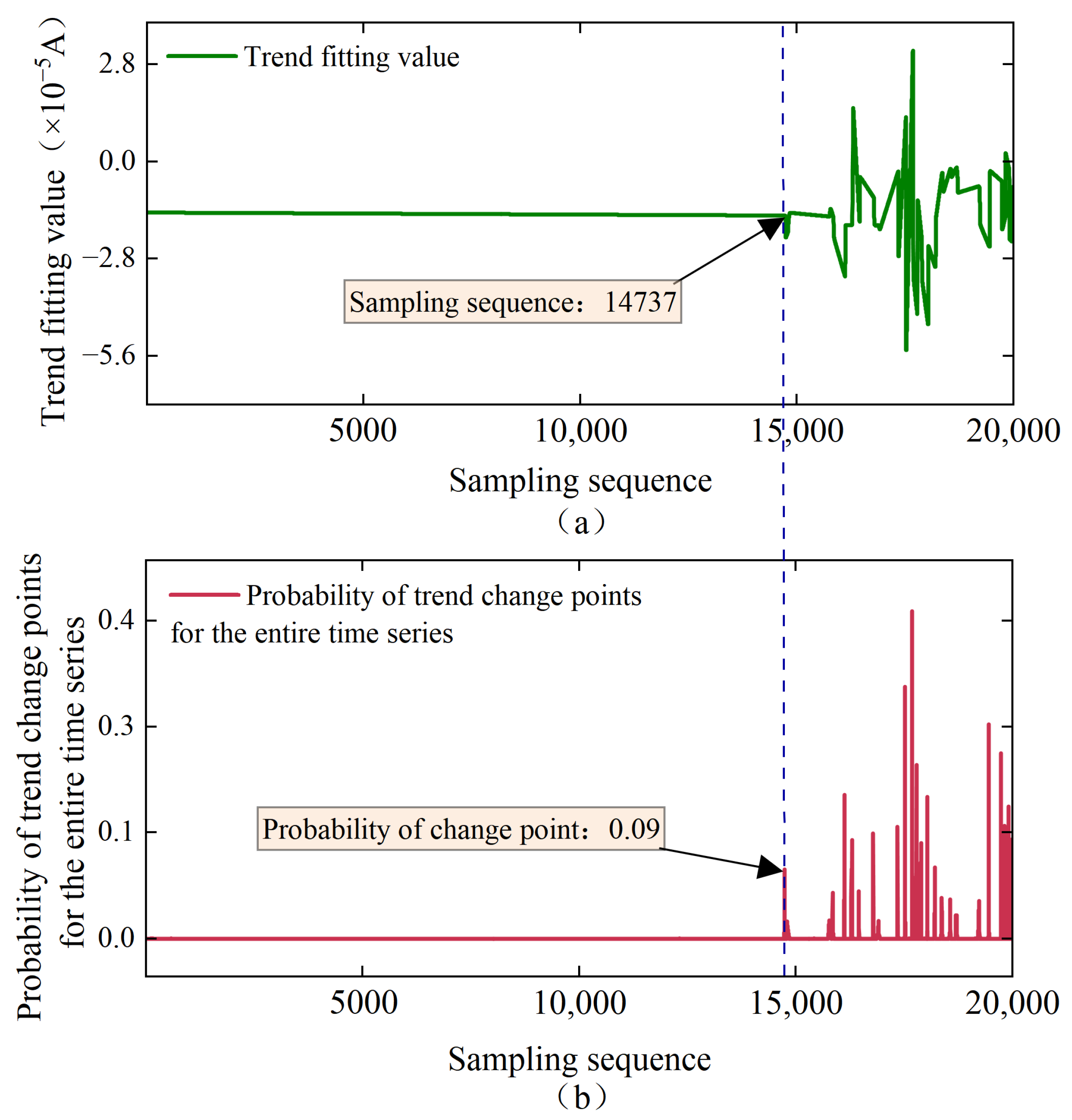
- The posterior change-point probability exhibits a distinct local peak;
- (2)
- The fitted trend before and after the candidate position shows an evident level or slope change;
- (3)
- The trend variation persists over the subsequent sampling interval rather than appearing as an isolated transient fluctuation.
2.2. Segment-Wise Signal Decomposition
2.3. Dominant-Component Identification and Adaptive Filtering
2.4. Breakpoint Smoothing and Continuity Preservation
2.5. Trend-Component Prediction and Signal Reconstruction
2.6. Evaluation Indexes for Reconstruction Effect of Rotor Current Signal
2.7. Implementation Procedure
| Algorithm 1. The BEAST-based segmented denoising of maglev gyro rotor current signals. |
Input: Raw rotor current sequence .
|
3. Results and Discussion
3.1. Experimental Site, Instrument, and Data Acquisition
3.2. Data Preprocessing and Parameter Configuration
3.3. Representative Signal-Processing Results
3.4. Comparative Performance on All Test Signals
3.5. Ablation Study
- Original data scheme.
- Baseline model (EMD + MAF + ARIMA).
- Baseline model integrated with the BEAST module (BEAST + EMD + MAF + ARIMA).
- Baseline model integrated with the OWT module (EMD + OWT + -MAF + ARIMA).
- The complete proposed method integrating both BEAST and OWT modules.
4. Conclusions
- (1)
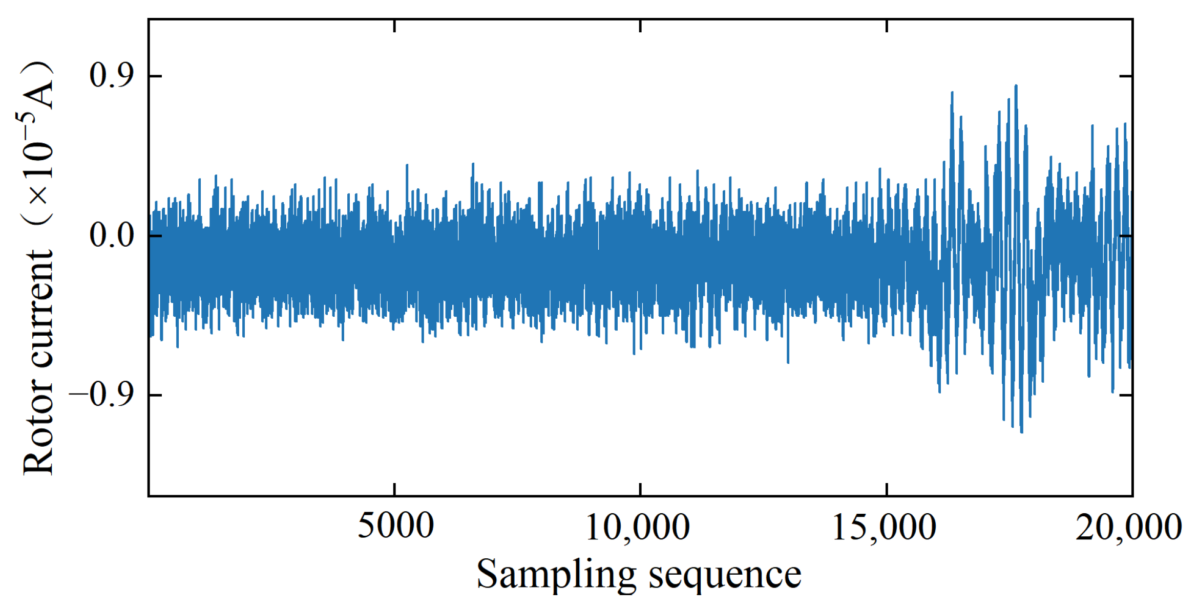
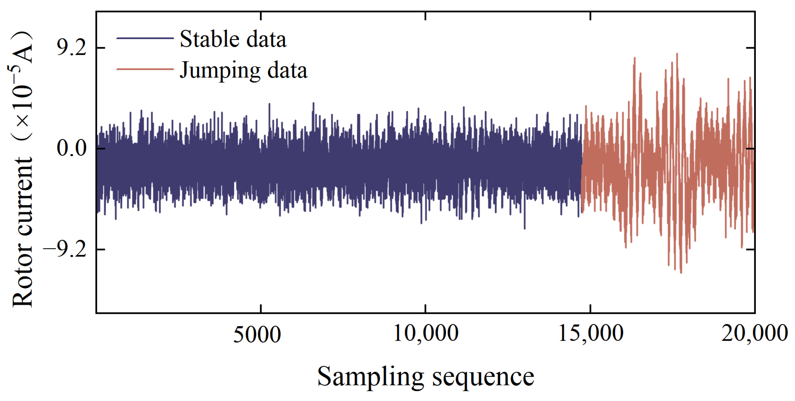
- BEAST enables adaptive localization of disturbance onset without manually defined segmentation windows. The rotor current sequence is divided into stationary and disturbed intervals according to posterior evidence of a persistent structural trend change. In the representative sequence, the disturbance boundary was identified at sample 14,737, while all 20,000 observations and their original temporal order were retained.
- (2)
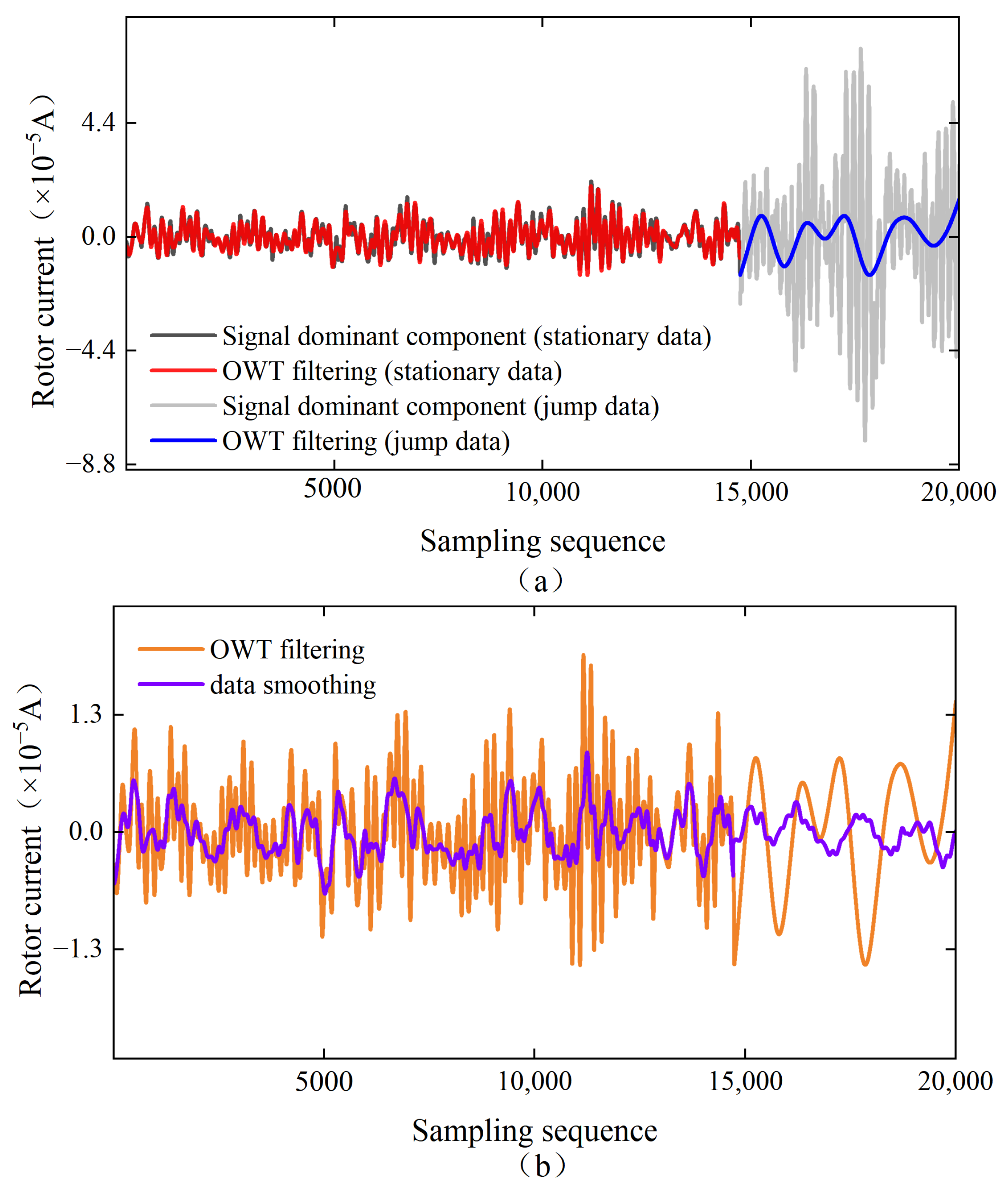
- Segment-wise processing reduces the parameter mismatch inherent in uniform denoising. Independent EMD and Hausdorff-distance-based IMF screening produced different component-removal orders for the stationary and jump intervals. Applying segment-specific wavelet decomposition levels therefore avoided excessive smoothing of the stationary interval and insufficient noise suppression in the strongly disturbed interval.
- (3)
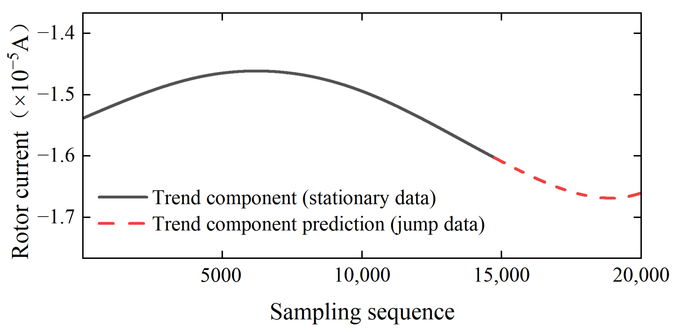
- The synergistic integration of global smoothing and trend forecasting ensures the continuity and integrity of the signal. Moving-average processing corrected the artificial discontinuity introduced at the segment junction, whereas ARIMA reconstructed the trend component of the disturbed interval from the stationary reference trend. Unlike sample-deletion methods, the proposed approach retained the complete sequence and preserved potentially useful azimuth-related information.
- (4)
- The proposed framework achieved consistent improvements in both signal stability and north-seeking accuracy. Across 12 field-collected sequences, the mean standard deviation decreased from 22.52 × 10⁻⁶ A to 6.54 × 10⁻⁶ A, corresponding to a reduction of 70.96%. The mean absolute azimuth error decreased from 8.30″ to 4.12″, representing an improvement of 50.36%. Valid azimuth results and error reductions were obtained for all 12 sequences, and the proposed method significantly outperformed OHHT, HSA-KS, and MAF-ARIMA in the paired statistical comparisons.
Author Contributions
Funding
Institutional Review Board Statement
Informed Consent Statement
Data Availability Statement
Acknowledgments
Conflicts of Interest
References
- Zhang, D.L.; Zhang, P.; Zhang, W.P.; He, B.N.; Zhu, G.L. A Weight Adaptive Kalman Information Fusion Method for Attitude Measurement. IEEE Sens. J. 2023, 23, 30683–30690. [Google Scholar] [CrossRef] [Scilit]
- Li, G.Q. Research on high-precision alignment control method for extra-long industrial rails. Acta Geod. Cartogr. Sin. 2023, 52, 869. [Google Scholar]
- Si, D.G.; Xiong, W.H.; Zhang, S.J.; Ma, Q.; Miao, P.P.; Liu, J.Q. Study on the estimation of lateral breakthrough error in horizontal control survey of super long tunnel. Bull. Surv. Mapp. 2024, 1, 155–160. [Google Scholar]
- Wang, Y.W. Research on the key processing technology of north-seeking non-stationary data measured by the maglevgyroscope. Acta Geod. Cartogr. Sin. 2025, 54, 2099. [Google Scholar]
- Li, X.J. Study on the Combined Adjustment Method of Azimuth Weighting of Maglev Gyro with Non-Equal Precision and Underground Conductor. Master’s Thesis, Chang’an University, Xi’an, China, 2024. [Google Scholar]
- Shi, P.X.; Yang, Z.Y.; Ji, G.F. Research on Data Processing Method of Maglev Gyroscope Based on Hilbert-Huang Transform. Bull. Surv. Mapp. 2015, 119–123. [Google Scholar]
- Gong, Y.; Yang, Z.; Shi, Z. Technical characteristics of GAT high accuracy magnetic suspension gyro station and application in mine surveying. Sci. Surv. Mapp. 2012, 37, 185–187. [Google Scholar]
- Shi, Z.; Yang, Z.; Ma, J. The detection method of maglev gyroscope abnormal data based on the characteristics of two positioning. Sci. Surv. Mapp. 2015, 40, 102–105+109. [Google Scholar]
- Liu, D.; Shi, Z.; Yang, Z.Y.; Zou, C.X. A Noise Reduction Method for Signal Reconstruction and Error Compensation of a Maglev Gyroscope Under Persistent External Interference. Sensors 2024, 24, 8005. [Google Scholar] [CrossRef] [Scilit] [PubMed]
- Wang, Y.W.; Yang, Z.Q.; Shi, Z.; Ma, J.; Liu, D.; Shi, L. Periodic error detection and separation of magnetic levitation gyroscope signals based on continuous wavelet transform and singular spectrum analysis. Meas. Sci. Technol. 2022, 33, 065107. [Google Scholar] [CrossRef] [Scilit]
- Ma, J. Research on Key Technology of Maglev Gyroscope Orientation Measurement for Super Long Tunnel Under Complex Environment. Ph.D. Thesis, Chang’an University, Xi’an, China, 2019. [Google Scholar]
- Wang, Y.W.; Yang, Z.Q.; Ma, J.; Shi, Z.; Liu, D.; Shi, L.; Li, H. A Novel Method for Automatic Detection and Elimination of the Jumps Caused by the Instantaneous Disturbance Torque in the Maglev Gyro Signal. Sensors 2023, 23, 2763. [Google Scholar] [CrossRef] [Scilit] [PubMed]
- Liu, D.; Shi, Z.; Zou, C.X.; Yang, Z.Y.; Li, J.F. A Novel Method for Noise Reduction and Jump Correction of Maglev Gyroscope Rotor Signals Under Instantaneous Perturbations. Sensors 2025, 25, 2131. [Google Scholar] [CrossRef] [Scilit] [PubMed]
- Zhao, K.G.; Wulder, M.A.; Hu, T.X.; Bright, R.; Wu, Q.S.; Qin, H.M.; Li, Y.; Toman, E.; Mallick, B.; Zhang, X.S.; et al. Detecting change-point, trend, and seasonality in satellite time series data to track abrupt changes and nonlinear dynamics: A Bayesian ensemble algorithm. Remote Sens. Environ. 2019, 232, 111181. [Google Scholar] [CrossRef] [Scilit]
- Granata, F.; Di Nunno, F. Evolving drought dynamics in Barcelona: Leveraging a Bayesian ensemble algorithm for insightful analysis and a bidirectional long short-term memory network for predictive modeling. Stoch. Environ. Res. Risk Assess. 2025, 39, 1253–1270. [Google Scholar] [CrossRef] [Scilit]
- Sahu, D.; Dewangan, R.K.; Matharu, S.P.S. Long short-term memory based fault diagnosis of rolling element bearings using vibration signals. J. Vib. Control 2026, 32, 2116–2127. [Google Scholar] [CrossRef] [Scilit]
- Yang, Z.H.; Dong, Q.J.; Zhang, X.; Zhu, H.Y.; Cheng, Z.T. Development of a Two-Stage LSTM for Multi-Step Runoff Forecasting Using a XAJ Model and EEMD. Water Resour. Manag. 2026, 40, 81. [Google Scholar] [CrossRef] [Scilit]
- Zarichnyi, M.; Berezsky, O.; Berezkyi, M.; Teslyuk, V. Method and Algorithms for Computing Fuzzy Fréchet and Hausdorff Distance. Mathematics 2026, 14, 892. [Google Scholar] [CrossRef] [Scilit]
- Che, M.; Perales, R.; Sormani, C. Gromov’s compactness theorem for the intrinsic timed-Hausdorff distance. Differ. Geom. Appl. 2026, 103, 102364. [Google Scholar] [CrossRef] [Scilit]
- Liu, C.C.; Yang, Z.Q.; Shi, Z.; Ma, J.; Cao, J. A Gyroscope Signal Denoising Method Based on Empirical Mode Decomposition and Signal Reconstruction. Sensors 2019, 19, 5064. [Google Scholar] [CrossRef] [Scilit] [PubMed]
- Liu, Z.M.; Tang, J.C.; Li, B.G.; Li, Y.H.; Yang, F.Z. Research on Denoising Methods for Infrasound Leakage Signals Using Improved Wavelet Threshold Algorithm. Machines 2025, 13, 1062. [Google Scholar] [CrossRef] [Scilit]
- Führ, H.; Getter, M. Energy propagation in scattering convolution networks can be arbitrarily slow. Appl. Comput. Harmon. Anal. 2025, 79, 101790. [Google Scholar] [CrossRef] [Scilit]
- Ma, J.; Yang, Z.Q.; Shi, Z.; Zhang, X.W.; Liu, C.C. Application and Optimization of Wavelet Transform Filter for North-Seeking Gyroscope Sensor Exposed to Vibration. Sensors 2019, 19, 3624. [Google Scholar] [CrossRef] [Scilit] [PubMed]
- Zhang, P.X.; Wang, J.R.; Zhu, Y.Q. Research on Equidistant Control of Robotic Arm for Complex Surface Cleaning. J. Rob. 2026, 2026, 1348108. [Google Scholar] [CrossRef] [Scilit]
- Felix, V.A.R.; Rohani, P.; Drake, J.M. A single autoregressive integrated moving average with exogenous variable outperforms ensembles of autoregressive models for forecasting influenza hospitalizations in the contiguous United States. J. R. Soc. Interface 2026, 23, 20250813. [Google Scholar] [CrossRef] [Scilit] [PubMed]
- Elbatal, I.; Almetwally, E.M.; Alaskar, M.Z.; Alsaedi, B.S.O.; Alzubaidi, S.; Yusuf, M. Predictive analytics in accounting: Using regression models to forecast financial outcomes. Alex. Eng. J. 2025, 128, 484–492. [Google Scholar] [CrossRef] [Scilit]
- Chaipitak, S.; Choopradit, B. Arima for Forecasting the Exchange Rate of the Thai Baht Against the Chinese Yuan. Adv. Appl. Stat. 2023, 84, 51–64. [Google Scholar] [CrossRef] [Scilit]
- Kabbilawsh, P.; Kumar, D.S.; Chithra, N.R. Forecasting long-term monthly precipitation using SARIMA models. J. Earth Syst. Sci. 2022, 131, 174. [Google Scholar] [CrossRef] [Scilit]
- Fahmi, A.; Kashyzadeh, K.R.; Ghorbani, S. Enhanced Autoregressive Integrated Moving Average Model for Anomaly Detection in Power Plant Operations. Int. J. Eng. 2024, 37, 1691–1699. [Google Scholar] [CrossRef] [Scilit]
- Zhuang, J.C.; Cao, Y.D.; Ding, Y.F.; Jia, M.P.; Feng, K. An autoregressive model-based degradation trend prognosis considering health indicators with multiscale attention information. Eng. Appl. Artif. Intell. 2024, 131, 107868. [Google Scholar] [CrossRef] [Scilit]




| Module | Parameter | Value/Rationale |
|---|---|---|
| Implementation | Software environment | MATLAB R2024b with the Rbeast toolbox |
| BEAST | Seasonal component | Disabled (no significant periodicity observed in the rotor current) |
| Truncated Poisson prior | λ = 0.5 × N × 10−4 (N = 20,000) | |
| MCMC iterations/Burn-in | 10,000/2000 | |
| Remaining Bayesian priors | Default configuration of the official Rbeast implementation | |
| EMD | Decomposition stopping criterion | Residual becomes monotonic or contains no more than one extremum |
| Hausdorff-based IMF selection | IMF identification criterion | PDF similarity based on the Hausdorff distance (Equation (9)) |
| OWT (Stationary interval) | Wavelet basis/Decomposition level | sym10/6 |
| OWT (Jump interval) | Wavelet basis/Decomposition level | sym10/9 |
| OWT (Common settings) | Threshold selection/Thresholding | rigrsure/Soft threshold |
| Moving-average smoothing | Window length | 500 samples |
| ARIMA | Model order selection | Determined using the ADF and KPSS stationarity tests together with the AIC–BIC criterion |
| Item | Configuration |
|---|---|
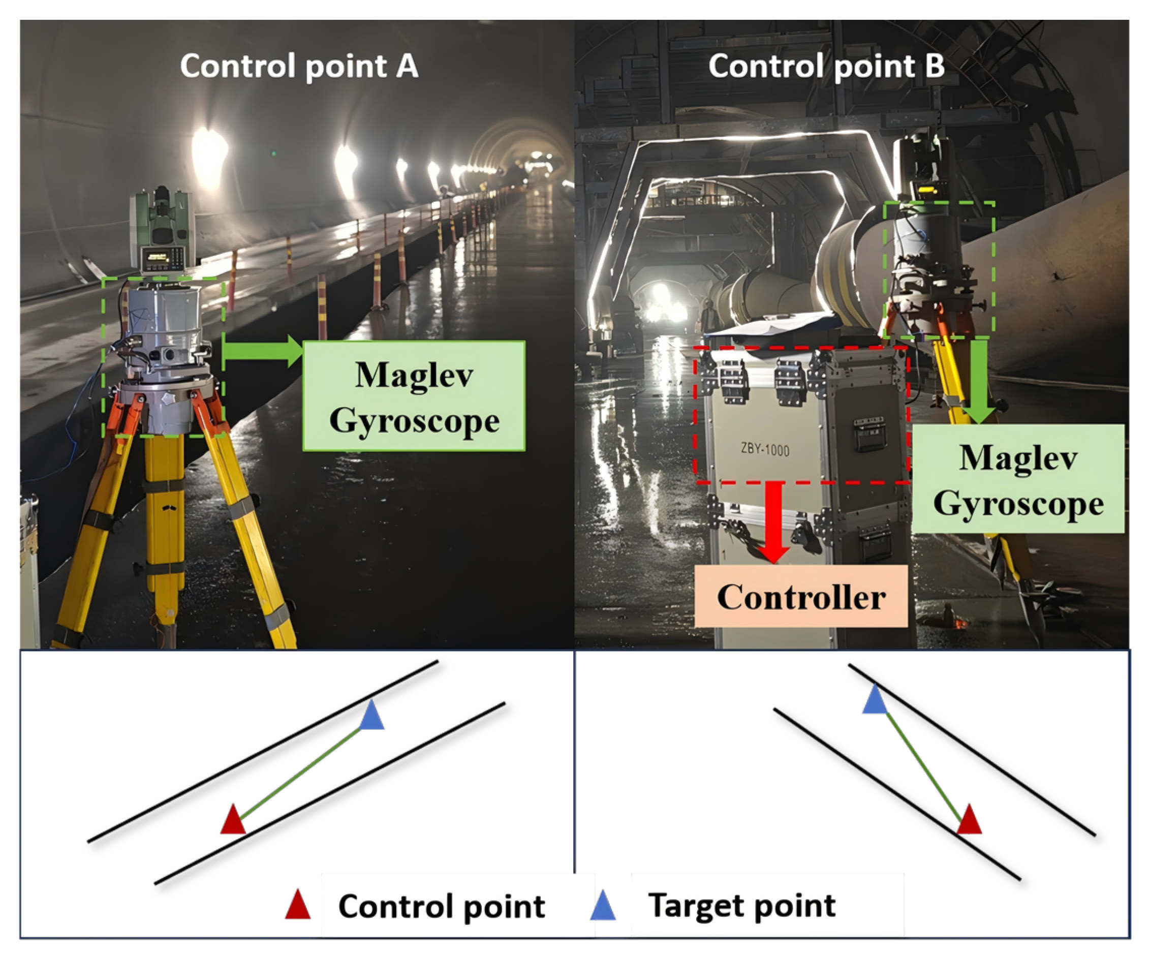
| Test environment | Railway tunnel |
| Observation sites | Control Points A and B |
| Instrument model | GAT D05 |
| Nominal north-seeking accuracy | 5.0″ |
| Sampling frequency | 167 Hz |
| Sampling duration | 120 s |
| Samples per sequence | 20,000 |
| Number of sequences | 12 |
| Rotor current unit | A |
| Reference azimuth accuracy | Better than 1.2″ |
| Main disturbance sources | Vehicles, airflow, personnel, and engineering machinery |
| Method | Parameter | Value/Rationale |
|---|---|---|
| OHHT | EMD reconstruction order | 8 |
| Wavelet basis | db4 | |
| Wavelet decomposition level | 4 | |
| Threshold selection | heursure | |
| HSA-KS | Segmentation significance level | 0.05 |
| Kolmogorov–Smirnov confidence level | 95% | |
| Minimum segmentation window | 100 samples | |
| MAF-ARIMA | Moving-average window length | 500 samples |
| ARIMA model order | Determined using the AIC–BIC criterion |
| IMF Component | 1 | 2 | 3 | 4 | 5 |
| HD1 (×103) | 7.88 | 44.46 | 79.08 | 113.43 | 84.25 |
| HD2 (×103) | 8.17 | 45.02 | 81.54 | 50.98 | 0.64 |
| IMF Component | 6 | 7 | 8 | 9 | 10 |
| HD1 (×103) | 120.40 | 190.45 | 356.41 | 1349.62 | 697.92 |
| HD2 (×103) | 75.23 | 17.26 | 78.08 | 348.55 | /— |
| Signal Group | RAW | OHHT | HSA-KS | MAF-ARIMA | Proposed Method |
|---|---|---|---|---|---|
| 1 | 19.72 | 1.13 | 14.71 | 4.29 | 2.89 |
| 2 | 13.48 | 1.86 | 12.35 | 2.83 | 4.26 |
| 3 | 17.03 | 11.61 | 14.74 | 9.70 | 4.28 |
| 4 | 18.52 | 16.34 | 12.55 | 7.83 | 4.10 |
| 5 | 24.34 | 22.59 | 16.38 | 10.07 | 5.07 |
| 6 | 15.91 | 3.77 | 15.30 | 3.21 | 3.44 |
| 7 | 16.37 | 5.79 | 16.22 | 5.82 | 6.27 |
| 8 | 35.51 | 34.30 | 21.95 | 21.01 | 13.21 |
| 9 | 25.76 | 11.84 | 17.86 | 9.57 | 7.36 |
| 10 | 38.54 | 29.34 | 27.34 | 20.55 | 14.57 |
| 11 | 24.75 | 15.69 | 19.13 | 10.51 | 7.80 |
| 12 | 20.34 | 12.11 | 14.72 | 8.54 | 5.23 |
| Mean | 22.52 | 13.86 | 16.94 | 9.49 | 6.54 |
| Improvement (%) | — | 38.45 | 24.78 | 57.86 | 70.96 |
| Signal Group | RAW | OHHT | HSA-KS | MAF-ARIMA | Proposed Method |
|---|---|---|---|---|---|
| 1 | 7.03 | 3.74 | 5.26 | 4.60 | 2.83 |
| 2 | 3.49 | 3.47 | / | / | 2.50 |
| 3 | 13.81 | 13.46 | 5.73 | 5.56 | 5.43 |
| 4 | 3.60 | 3.56 | 2.75 | 2.94 | 1.67 |
| 5 | 7.85 | 7.15 | 6.74 | 6.88 | 4.17 |
| 6 | 10.11 | 6.59 | 9.09 | 5.72 | 3.93 |
| 7 | 8.47 | 7.64 | / | 5.68 | 4.17 |
| 8 | 7.44 | 7.21 | 6.97 | 5.86 | 5.40 |
| 9 | 7.42 | 6.92 | 6.57 | 5.58 | 4.71 |
| 10 | 13.65 | 9.56 | 8.53 | 8.26 | 6.34 |
| 11 | 9.65 | 7.62 | 7.15 | 5.91 | 5.11 |
| 12 | 7.03 | 6.29 | 5.76 | 5.48 | 3.23 |
| Mean | 8.30 | 6.93 | 6.46 | 5.68 | 4.12 |
| Valid n | — | 12 | 10 | 11 | 12 |
| Improvement (%) | — | 16.51 | 22.17 | 31.57 | 50.36 |
| Method | n | Mean ± SD | Median (IQR) |
|---|---|---|---|
| RAW | 12 | 22.52 ± 7.78 | 20.03 (8.14) |
| OHHT | 12 | 13.86 ± 10.57 | 11.98 (12.62) |
| HSA-KS | 12 | 16.94 ± 4.24 | 15.76 (3.47) |
| MAF-ARIMA | 12 | 9.49 ± 5.91 | 9.06 (4.74) |
| Proposed method | 12 | 6.54 ± 3.75 | 5.15 (3.25) |
| Method | Valid n | Mean ± SD | Median (IQR) |
|---|---|---|---|
| RAW | 12 | 8.30 ± 3.22 | 7.65 (2.74) |
| OHHT | 12 | 6.93 ± 2.77 | 7.04 (1.97) |
| HSA-KS | 10 | 6.46 ± 1.77 | 6.66 (1.37) |
| MAF-ARIMA | 11 | 5.68 ± 1.30 | 5.68 (0.37) |
| Proposed method | 12 | 4.12 ± 1.37 | 4.17 (2.05) |
| Outcome | Comparison | Paired n | Raw p | Holm-Adjusted p |
|---|---|---|---|---|
| SD | Proposed method vs. RAW | 12 | <0.001 | 0.002 |
| SD | Proposed method vs. OHHT | 12 | 0.016 | 0.019 |
| SD | Proposed method vs. HSA-KS | 12 | <0.001 | 0.002 |
| SD | Proposed method vs. MAF-ARIMA | 12 | 0.009 | 0.019 |
| D | Proposed method vs. RAW | 12 | <0.001 | 0.002 |
| D | Proposed method vs. OHHT | 12 | <0.001 | 0.002 |
| D | Proposed method vs. HSA-KS | 10 | 0.002 | 0.002 |
| D | Proposed method vs. MAF-ARIMA | 11 | <0.001 | 0.002 |
| Scheme | Error Mean (″) | Error Improv. (%) | Std Mean (×10−6 A) | Std Improv. (%) | Jump Mean (×10−6 A) | Jump Improv. (%) |
|---|---|---|---|---|---|---|
| A | 8.30 | — | 22.52 | — | 18.80 | — |
| B | 5.68 | 31.57 | 9.49 | 57.86 | 1.06 | 94.34 |
| C | 4.69 | 43.49 | 7.90 | 65.04 | 0.83 | 95.58 |
| D | 5.02 | 39.52 | 8.59 | 62.00 | 0.89 | 95.24 |
| E | 4.12 | 50.36 | 6.54 | 70.96 | 0.71 | 96.22 |
| Scheme | Group | Error (″) | Std (×10−6 A) | Breakpoint Jump (A) | Group | Error (″) | Std (×10−6 A) | Breakpoint Jump (A) |
|---|---|---|---|---|---|---|---|---|
| A | G1 | 7.03 | 19.72 | 1.70 × 10⁻⁵ | G2 | 3.49 | 13.48 | 8.00 × 10⁻⁶ |
| B | 4.60 | 4.29 | 2.88 × 10⁻⁸ | / | 2.83 | 9.58 × 10⁻⁸ | ||
| C | 3.17 | 3.63 | 1.21 × 10⁻⁸ | 2.92 | 4.34 | 3.73 × 10⁻⁸ | ||
| D | 3.85 | 3.91 | 2.05 × 10⁻⁸ | 2.97 | 4.01 | 6.12 × 10⁻⁸ | ||
| E | 2.83 | 2.89 | 2.03 × 10⁻⁹ | 2.50 | 4.26 | 5.47 × 10⁻⁹ | ||
| A | G3 | 13.81 | 17.03 | 3.00 × 10⁻⁶ | G4 | 3.6 | 18.52 | −3.00 × 10⁻⁶ |
| B | 5.56 | 9.70 | 5.04 × 10⁻⁸ | 2.94 | 7.83 | −2.54 × 10⁻⁸ | ||
| C | 5.48 | 4.41 | 1.83 × 10⁻⁸ | 2.53 | 4.27 | −1.10 × 10⁻⁸ | ||
| D | 5.52 | 6.15 | 3.11 × 10⁻¹⁰ | 2.78 | 5.92 | −1.86 × 10⁻⁸ | ||
| E | 5.43 | 4.28 | 6.85 × 10⁻⁶ | 1.67 | 4.10 | −1.76 × 10⁻⁹ | ||
| A | G5 | 7.85 | 24.34 | 1.00 × 10⁻⁶ | G6 | 10.11 | 15.91 | −3.10 × 10⁻⁵ |
| B | 6.88 | 10.07 | 7.92 × 10⁻⁸ | 5.72 | 3.21 | −1.15 × 10⁻⁵ | ||
| C | 4.93 | 5.23 | 9.39 × 10⁻⁸ | 4.54 | 3.52 | −9.06 × 10⁻⁶ | ||
| D | 5.65 | 7.14 | 5.08 × 10⁻⁸ | 5.16 | 4.05 | −9.82 × 10⁻⁶ | ||
| E | 4.17 | 5.07 | 3.34 × 10⁻⁸ | 3.93 | 3.44 | −8.31 × 10⁻⁶ | ||
| A | G7 | 8.47 | 16.37 | −2.80 × 10⁻⁵ | G8 | 7.44 | 35.51 | −5.70 × 10⁻⁵ |
| B | 5.68 | 5.82 | −9.11 × 10⁻⁸ | 5.86 | 21.01 | −2.62 × 10⁻⁷ | ||
| C | 5.11 | 6.99 | −7.43 × 10⁻⁸ | 5.55 | 19.77 | −1.71 × 10⁻⁷ | ||
| D | 5.32 | 6.35 | −6.47 × 10⁻⁸ | 5.61 | 20.40 | −2.05 × 10⁻⁷ | ||
| E | 4.17 | 6.27 | −1.80 × 10⁻⁸ | 5.4 | 13.29 | −3.43 × 10⁻⁸ | ||
| A | G9 | 7.42 | 25.76 | −1.60 × 10⁻⁵ | G10 | 13.65 | 38.54 | −2.03 × 10⁻⁶ |
| B | 5.58 | 9.57 | −4.62 × 10⁻⁷ | 8.26 | 20.55 | −4.39 × 10⁻⁸ | ||
| C | 5.09 | 8.84 | −3.18 × 10⁻⁷ | 6.98 | 18.48 | −1.87 × 10⁻⁸ | ||
| D | 5.31 | 9.12 | −3.47 × 10⁻⁷ | 7.45 | 19.23 | −2.64 × 10⁻⁸ | ||
| E | 4.71 | 7.36 | −9.71 × 10⁻⁸ | 6.34 | 14.62 | −4.89 × 10⁻⁹ | ||
| A | G11 | 9.65 | 24.75 | 4.40 × 10⁻⁵ | G12 | 7.03 | 20.34 | 1.70 × 10⁻⁵ |
| B | 5.91 | 10.51 | 6.27 × 10⁻⁸ | 5.48 | 8.54 | 4.12 × 10⁻⁸ | ||
| C | 5.37 | 8.42 | 7.16 × 10⁻⁸ | 4.62 | 7.05 | 6.74 × 10⁻⁸ | ||
| D | 5.64 | 9.26 | 4.05 × 10⁻⁸ | 4.96 | 7.61 | 2.93 × 10⁻⁸ | ||
| E | 5.11 | 7.80 | −9.87 × 10⁻⁹ | 3.23 | 5.23 | 1.36 × 10⁻⁸ |
Disclaimer/Publisher’s Note: The statements, opinions and data contained in all publications are solely those of the individual author(s) and contributor(s) and not of MDPI and/or the editor(s). MDPI and/or the editor(s) disclaim responsibility for any injury to people or property resulting from any ideas, methods, instructions or products referred to in the content. |
© 2026 by the authors. Licensee MDPI, Basel, Switzerland. This article is an open access article distributed under the terms and conditions of the Creative Commons Attribution (CC BY) license.
Share and Cite
Guo, B.; Shi, Z.; Liu, D.; Hu, X.; Jiang, G.; Dang, T. A Denoising Algorithm for Maglev Gyro Jump Data Based on Bayesian Ensemble Time-Series Segmentation. Sensors 2026, 26, 5287. https://doi.org/10.3390/s26165287
Guo B, Shi Z, Liu D, Hu X, Jiang G, Dang T. A Denoising Algorithm for Maglev Gyro Jump Data Based on Bayesian Ensemble Time-Series Segmentation. Sensors. 2026; 26(16):5287. https://doi.org/10.3390/s26165287
Chicago/Turabian StyleGuo, Binqiang, Zhen Shi, Di Liu, Xinkang Hu, Gang Jiang, and Tao Dang. 2026. "A Denoising Algorithm for Maglev Gyro Jump Data Based on Bayesian Ensemble Time-Series Segmentation" Sensors 26, no. 16: 5287. https://doi.org/10.3390/s26165287
APA StyleGuo, B., Shi, Z., Liu, D., Hu, X., Jiang, G., & Dang, T. (2026). A Denoising Algorithm for Maglev Gyro Jump Data Based on Bayesian Ensemble Time-Series Segmentation. Sensors, 26(16), 5287. https://doi.org/10.3390/s26165287