Figure 1.
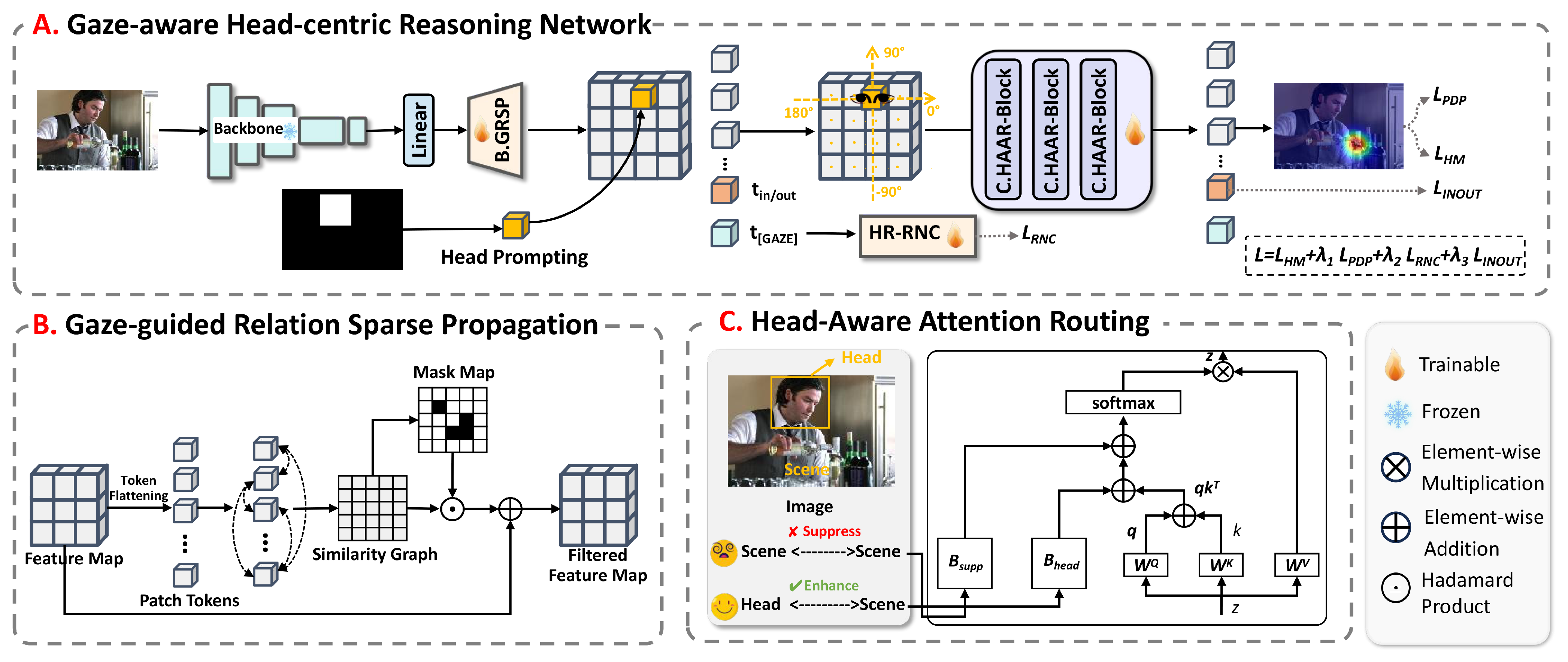
Overall architecture of the proposed GazeHRNet framework. (A) The full pipeline: a frozen DINOv2 backbone extracts patch features, which are processed by GRSP, conditioned with Head Prompting and HCPE, and processed by stacked HAAR blocks to produce gaze heatmap, patch distribution, and in/out predictions. The [GAZE] token receives HR-RNC constraints during training. (B) Gaze-guided Relation Soft Propagation: content-dependent similarity gating suppresses task-irrelevant token connections before the Transformer. (C) Head-Aware Attention Routing: head-guided bias enhances head-scene attention flow, while suppression bias penalizes nearby background interactions.
Figure 1.
Overall architecture of the proposed GazeHRNet framework. (A) The full pipeline: a frozen DINOv2 backbone extracts patch features, which are processed by GRSP, conditioned with Head Prompting and HCPE, and processed by stacked HAAR blocks to produce gaze heatmap, patch distribution, and in/out predictions. The [GAZE] token receives HR-RNC constraints during training. (B) Gaze-guided Relation Soft Propagation: content-dependent similarity gating suppresses task-irrelevant token connections before the Transformer. (C) Head-Aware Attention Routing: head-guided bias enhances head-scene attention flow, while suppression bias penalizes nearby background interactions.
Figure 2.
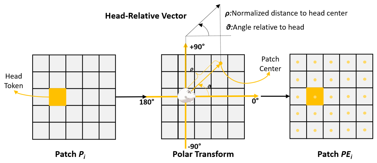
Illustration of Head-Centric Polar Encoding. For each patch , HCPE computes the angle and normalized distance relative to the head center, and encodes them into a per-patch positional embedding via multi-frequency sinusoidal functions.
Figure 2.
Illustration of Head-Centric Polar Encoding. For each patch , HCPE computes the angle and normalized distance relative to the head center, and encodes them into a per-patch positional embedding via multi-frequency sinusoidal functions.
Figure 3.
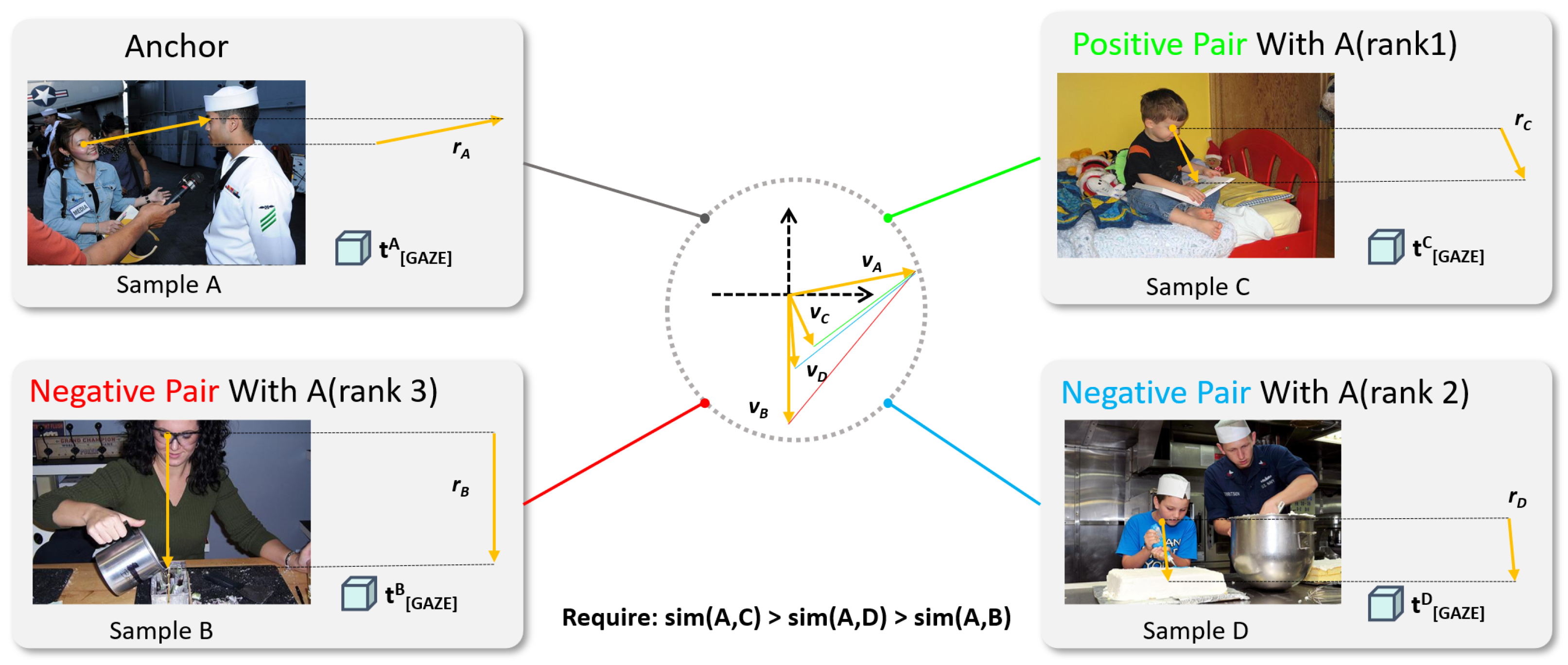
Illustration of Head-Relative Rank-N-Contrast Learning. Each sample’s head-relative gaze vector r defines its position in the label space. For anchor A, samples are ranked by label distance: C (rank 1) has the most similar gaze vector, followed by D (rank 2) and B (rank 3). The RnC loss requires feature similarity to preserve this ordering.
Figure 3.
Illustration of Head-Relative Rank-N-Contrast Learning. Each sample’s head-relative gaze vector r defines its position in the label space. For anchor A, samples are ranked by label distance: C (rank 1) has the most similar gaze vector, followed by D (rank 2) and B (rank 3). The RnC loss requires feature similarity to preserve this ordering.
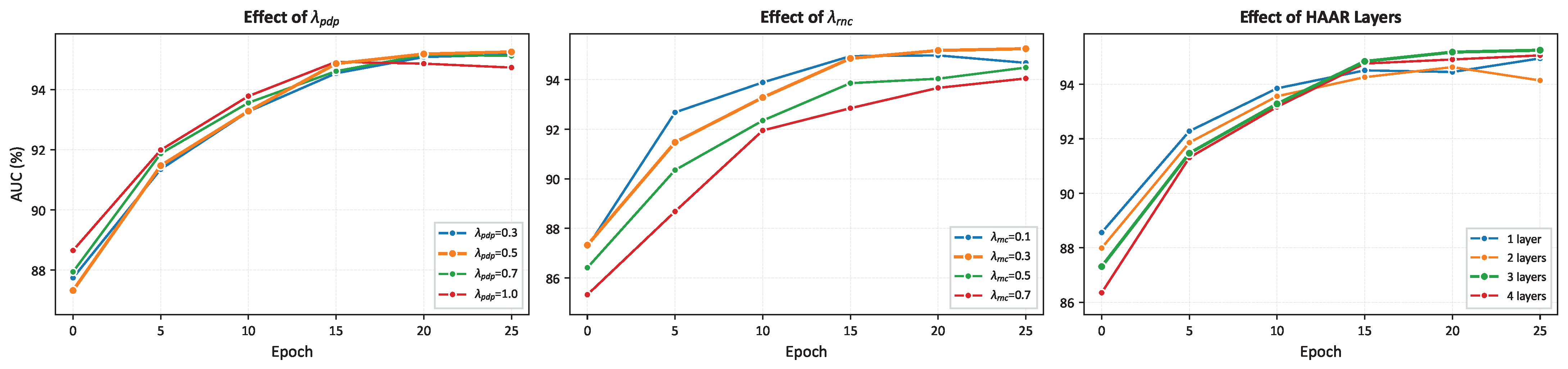
Figure 4.
Hyperparameter sensitivity analysis on GazeFollow. Left: effect of PDP loss weight ; achieves the best final AUC, while larger weights accelerate early convergence but cause late-stage degradation. Middle: effect of HR-RNC loss weight ; the model is more sensitive to this parameter, with best balancing representation structure and localization accuracy. Right: effect of the number of HAAR Transformer layers; three layers yield the best trade-off between capacity and optimization efficiency.
Figure 4.
Hyperparameter sensitivity analysis on GazeFollow. Left: effect of PDP loss weight ; achieves the best final AUC, while larger weights accelerate early convergence but cause late-stage degradation. Middle: effect of HR-RNC loss weight ; the model is more sensitive to this parameter, with best balancing representation structure and localization accuracy. Right: effect of the number of HAAR Transformer layers; three layers yield the best trade-off between capacity and optimization efficiency.
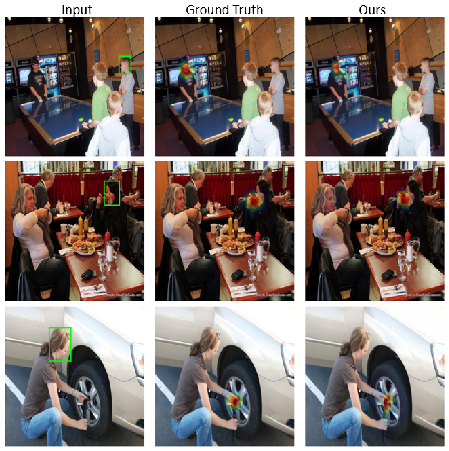
Figure 5.
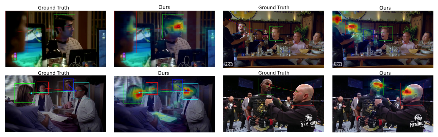
Qualitative results on GazeFollow. Each row shows one example. Left: input image with the target person’s head marked by a green bounding box. Middle: ground-truth gaze heatmap. Right: GazeHRNet prediction. For both ground-truth and predictions, red circles indicate the annotated/predicted gaze target locations, while the overlaid colored heatmaps visualize the probability distributions. The model accurately localizes gaze targets in multi-person, cluttered, and object-interaction scenarios.
Figure 5.
Qualitative results on GazeFollow. Each row shows one example. Left: input image with the target person’s head marked by a green bounding box. Middle: ground-truth gaze heatmap. Right: GazeHRNet prediction. For both ground-truth and predictions, red circles indicate the annotated/predicted gaze target locations, while the overlaid colored heatmaps visualize the probability distributions. The model accurately localizes gaze targets in multi-person, cluttered, and object-interaction scenarios.
Figure 6.
Qualitative generalization results of GazeHRNet in challenging real-world environments. In each image, colored bounding boxes denote the detected heads of different subjects, and the corresponding solid lines of the same color point from the head center to their predicted gaze target locations (highlighted by the overlaid heatmaps). The model successfully infers gaze targets in scenarios involving severe head occlusions (top-left), complex multi-person social interactions (top-right and bottom-left), and dynamic sporting events with intense mutual focus (bottom-right).
Figure 6.
Qualitative generalization results of GazeHRNet in challenging real-world environments. In each image, colored bounding boxes denote the detected heads of different subjects, and the corresponding solid lines of the same color point from the head center to their predicted gaze target locations (highlighted by the overlaid heatmaps). The model successfully infers gaze targets in scenarios involving severe head occlusions (top-left), complex multi-person social interactions (top-right and bottom-left), and dynamic sporting events with intense mutual focus (bottom-right).
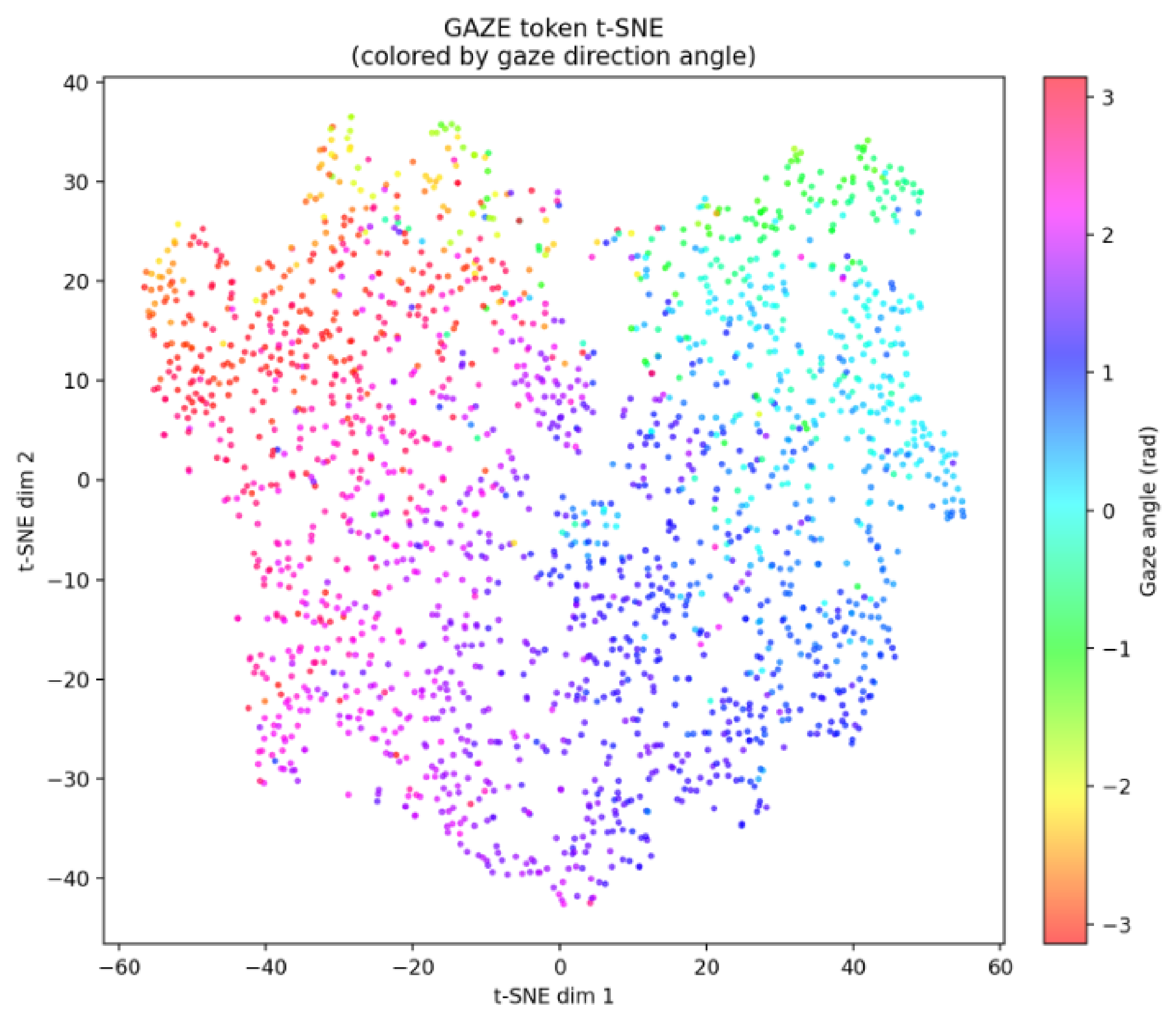
Figure 7.
t-SNE visualization of [GAZE] token features on the GazeFollow test set, colored by head-relative gaze direction angle (in radians). The smooth color gradient from left-looking (warm) to right-looking (cool) indicates that HR-RNC organizes the feature space according to gaze direction rather than absolute position.
Figure 7.
t-SNE visualization of [GAZE] token features on the GazeFollow test set, colored by head-relative gaze direction angle (in radians). The smooth color gradient from left-looking (warm) to right-looking (cool) indicates that HR-RNC organizes the feature space according to gaze direction rather than absolute position.
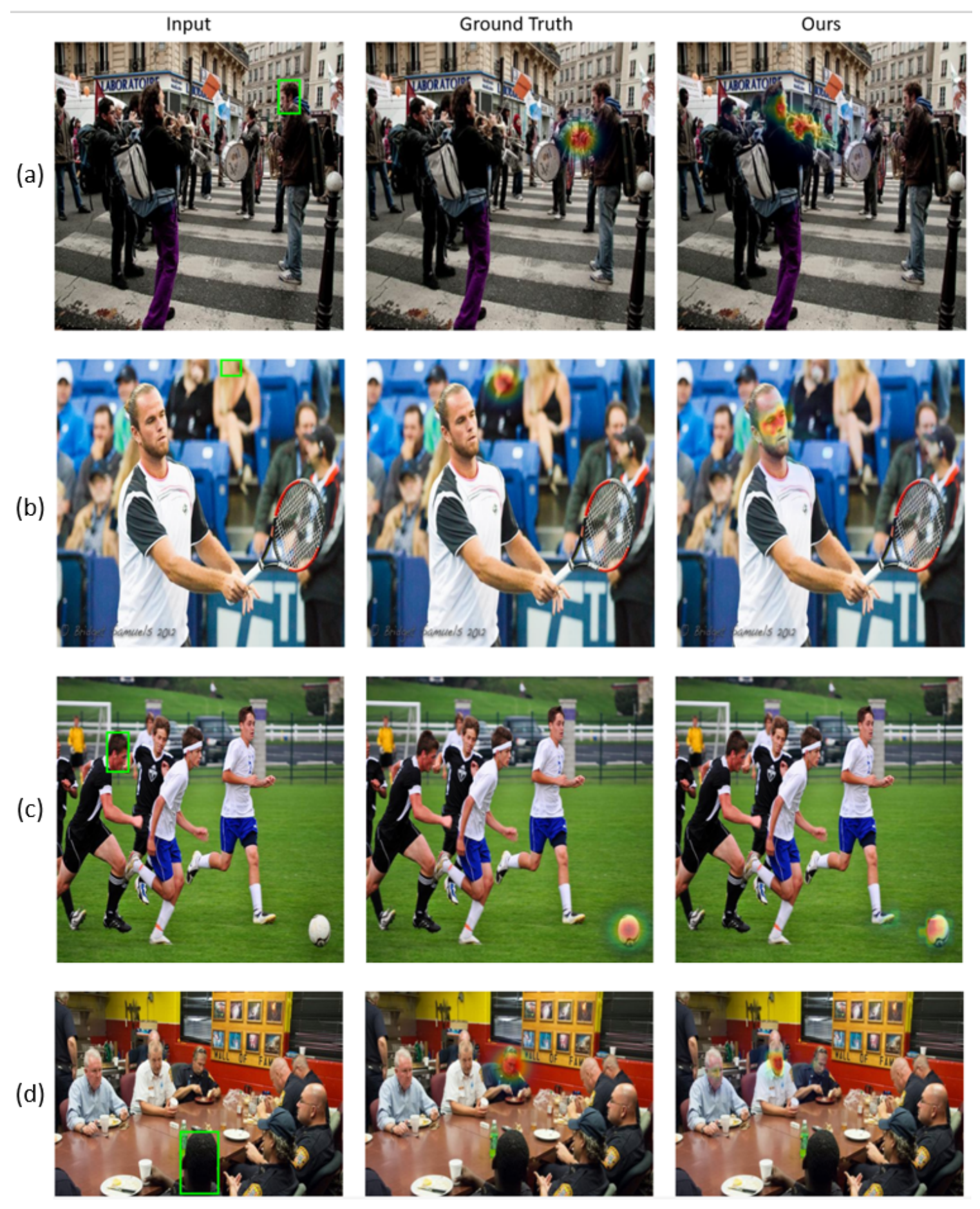
Figure 8.
Typical failure cases of GazeHRNet categorized into four scenarios. The three columns show the input image, the ground-truth gaze heatmap, and the gaze heatmap predicted by GazeHRNet, respectively. In the input images, the green rectangles indicate the head bounding boxes of the target persons. In the ground-truth and predicted heatmaps, warmer colors, such as red and yellow, indicate higher gaze likelihood, whereas cooler colors, such as green and blue, indicate lower gaze likelihood. The colored circular regions represent gaze heatmap responses rather than additional annotations. From top to bottom: (a) crowded scenes causing dispersed attention; (b) extremely small head regions leading to feature loss; (c) incorrect gaze direction estimation due to complex body posture; and (d) severe head occlusion forcing the model to over-rely on contextual guessing.
Figure 8.
Typical failure cases of GazeHRNet categorized into four scenarios. The three columns show the input image, the ground-truth gaze heatmap, and the gaze heatmap predicted by GazeHRNet, respectively. In the input images, the green rectangles indicate the head bounding boxes of the target persons. In the ground-truth and predicted heatmaps, warmer colors, such as red and yellow, indicate higher gaze likelihood, whereas cooler colors, such as green and blue, indicate lower gaze likelihood. The colored circular regions represent gaze heatmap responses rather than additional annotations. From top to bottom: (a) crowded scenes causing dispersed attention; (b) extremely small head regions leading to feature loss; (c) incorrect gaze direction estimation due to complex body posture; and (d) severe head occlusion forcing the model to over-rely on contextual guessing.
Table 1.
Comparison with state-of-the-art methods on GazeFollow and VideoAttentionTarget. All baseline methods report their fully trainable total parameters. For our GazeHRNet, we report the trainable parameters (3.0 M), while the total parameter count, including the frozen DINOv2 backbone, is 89.5 M. The Input column indicates auxiliary modalities: I = image, D = depth, P = pose, O = objects, E = eyes. Bold marks the best result and underline marks the second best. The up arrow (↑) indicates that higher values are better, and the down arrow (↓) indicates that lower values are better.
Table 1.
Comparison with state-of-the-art methods on GazeFollow and VideoAttentionTarget. All baseline methods report their fully trainable total parameters. For our GazeHRNet, we report the trainable parameters (3.0 M), while the total parameter count, including the frozen DINOv2 backbone, is 89.5 M. The Input column indicates auxiliary modalities: I = image, D = depth, P = pose, O = objects, E = eyes. Bold marks the best result and underline marks the second best. The up arrow (↑) indicates that higher values are better, and the down arrow (↓) indicates that lower values are better.
| | | | GazeFollow | VideoAttentionTarget |
|---|
| Method | Params | Input | AUC ↑ | Avg L2 ↓ | Min L2 ↓ | AUC ↑ | L2 ↓ | AP ↑ |
|---|
| One Human | – | – | 0.924 | 0.096 | 0.040 | 0.921 | 0.051 | 0.925 |
| SalGaze [8] | 50 M | I | 0.878 | 0.190 | 0.113 | – | – | – |
| GASE [44] | 51 M | I | 0.896 | 0.187 | 0.112 | 0.833 | 0.171 | 0.712 |
| GazeDir [9] | 55 M | I | 0.906 | 0.145 | 0.081 | – | – | – |
| DAT [11] | 61 M | I | 0.921 | 0.137 | 0.077 | 0.860 | 0.134 | 0.853 |
| JMCGaze [45] | 50 M | I | 0.908 | 0.136 | 0.074 | – | – | – |
| DualAttn [12] | 68 M | I+D+E | 0.922 | 0.124 | 0.067 | 0.905 | 0.108 | 0.896 |
| ESCNet [23] | 29 M | I+D+P | 0.928 | 0.122 | – | 0.885 | 0.120 | 0.869 |
| DepthGaze [14] | 52 M | I+D+P | 0.920 | 0.118 | 0.063 | 0.900 | 0.104 | 0.895 |
| MMACD [46] | 92 M | I+D | 0.927 | 0.141 | – | 0.862 | 0.125 | 0.742 |
| IAGaze [7] | 61 M | I+D+O | 0.923 | 0.128 | 0.069 | 0.880 | 0.118 | 0.881 |
| MMGaze [13] | 35 M | I+D+P | 0.943 | 0.114 | 0.056 | 0.914 | 0.110 | 0.879 |
| Gaze3D [47] | 46 M | I+D | 0.896 | 0.196 | 0.127 | 0.832 | 0.199 | 0.800 |
| PatchGaze [20] | 61 M | I+D | 0.934 | 0.123 | 0.065 | 0.917 | 0.109 | 0.908 |
| ChildPlay [48] | 25 M | I+D | 0.939 | 0.122 | 0.062 | 0.914 | 0.109 | 0.834 |
| Sharingan [24] | 135 M | I | 0.944 | 0.113 | 0.057 | – | 0.107 | 0.891 |
| GazeVLM [49] | – | I | 0.929 | 0.131 | 0.076 | 0.926 | 0.112 | 0.898 |
| GazeHRNet (Ours) | 3.0 M | I | 0.952 | 0.102 | 0.055 | 0.929 | 0.103 | 0.909 |
Table 2.
Cross-dataset evaluation. All models are trained on GazeFollow and tested directly on VAT, GOO-Real, and ChildPlay without fine-tuning. Bold marks the best result and underline marks the second best. The up arrow (↑) indicates that higher values are better, and the down arrow (↓) indicates that lower values are better.
Table 2.
Cross-dataset evaluation. All models are trained on GazeFollow and tested directly on VAT, GOO-Real, and ChildPlay without fine-tuning. Bold marks the best result and underline marks the second best. The up arrow (↑) indicates that higher values are better, and the down arrow (↓) indicates that lower values are better.
| | VAT | GOO-Real | ChildPlay |
|---|
| Method | AUC ↑ | L2 ↓ | AUC ↑ | L2 ↓ | AUC ↑ | L2 ↓ |
|---|
| DAT | 0.906 | 0.119 | 0.670 | 0.334 | 0.912 | 0.121 |
| DepthGaze | 0.900 | 0.104 | – | – | – | – |
| MMACD | – | – | 0.840 | 0.238 | – | – |
| PatchGaze | 0.923 | 0.109 | 0.869 | 0.202 | 0.933 | 0.113 |
| MMGaze | 0.907 | 0.137 | – | – | 0.923 | 0.142 |
| ChildPlay | 0.911 | 0.123 | – | – | 0.932 | 0.115 |
| GazeHRNet (Ours) | 0.928 | 0.103 | 0.892 | 0.173 | 0.939 | 0.109 |
Table 3.
Block-wise ablation study of GazeHRNet on GazeFollow. No. 1–3 verify head-centric spatial encoding. No. 4–9 verify gaze-aware feature interaction. No. 10–14 verify supervision and representation learning. Within each group, individual and complementary effects are evaluated using controlled module combinations. Bold marks the best result within each group and the overall best result. The up arrow (↑) indicates that higher values are better, and the down arrow (↓) indicates that lower values are better. The checkmark (✓) indicates the inclusion of a specific module.
Table 3.
Block-wise ablation study of GazeHRNet on GazeFollow. No. 1–3 verify head-centric spatial encoding. No. 4–9 verify gaze-aware feature interaction. No. 10–14 verify supervision and representation learning. Within each group, individual and complementary effects are evaluated using controlled module combinations. Bold marks the best result within each group and the overall best result. The up arrow (↑) indicates that higher values are better, and the down arrow (↓) indicates that lower values are better. The checkmark (✓) indicates the inclusion of a specific module.
| | HCPE | | HAAR | Supervision & Repr. | GazeFollow |
|---|
| No. | | | GRSP | [GAZE] | | | PDP | AHS | RnC | HR | AUC ↑ | Avg L2 ↓ | Min L2 ↓ |
|---|
| 0 | | | | | | | | | | | 0.876 | 0.245 | 0.187 |
| 1 | ✓ | | | | | | | | | | 0.884 | 0.226 | 0.164 |
| 2 | | ✓ | | | | | | | | | 0.881 | 0.231 | 0.169 |
| 3 | ✓ | ✓ | | | | | | | | | 0.895 | 0.209 | 0.145 |
| 4 | ✓ | ✓ | ✓ | | | | | | | | 0.904 | 0.193 | 0.132 |
| 5 | ✓ | ✓ | | ✓ | ✓ | | | | | | 0.913 | 0.181 | 0.116 |
| 6 | ✓ | ✓ | | ✓ | | ✓ | | | | | 0.908 | 0.187 | 0.123 |
| 7 | ✓ | ✓ | ✓ | ✓ | ✓ | | | | | | 0.923 | 0.168 | 0.099 |
| 8 | ✓ | ✓ | ✓ | ✓ | | ✓ | | | | | 0.918 | 0.174 | 0.107 |
| 9 | ✓ | ✓ | ✓ | ✓ | ✓ | ✓ | | | | | 0.929 | 0.154 | 0.086 |
| 10 | ✓ | ✓ | ✓ | ✓ | ✓ | ✓ | ✓ | | | | 0.933 | 0.145 | 0.078 |
| 11 | ✓ | ✓ | ✓ | ✓ | ✓ | ✓ | | ✓ | | | 0.935 | 0.137 | 0.075 |
| 12 | ✓ | ✓ | ✓ | ✓ | ✓ | ✓ | ✓ | ✓ | | | 0.939 | 0.126 | 0.071 |
| 13 | ✓ | ✓ | ✓ | ✓ | ✓ | ✓ | ✓ | ✓ | ✓ | | 0.944 | 0.114 | 0.066 |
| 14 | ✓ | ✓ | ✓ | ✓ | ✓ | ✓ | ✓ | ✓ | ✓ | ✓ | 0.952 | 0.102 | 0.055 |
Table 4.
Removal-from-full ablation analysis on the GazeFollow dataset. Each row represents the full model with the specified component(s) removed. Bold marks the best result. The up arrow (↑) indicates that higher values are better, and the down arrow (↓) indicates that lower values are better.
Table 4.
Removal-from-full ablation analysis on the GazeFollow dataset. Each row represents the full model with the specified component(s) removed. Bold marks the best result. The up arrow (↑) indicates that higher values are better, and the down arrow (↓) indicates that lower values are better.
| Configuration | AUC ↑ | Avg L2 ↓ | Min L2 ↓ |
|---|
| w/o HCPE | 0.938 | 0.125 | 0.075 |
| w/o GRSP | 0.942 | 0.115 | 0.071 |
| w/o HAAR | 0.932 | 0.137 | 0.090 |
| w/o PDP | 0.948 | 0.113 | 0.059 |
| w/o AHS | 0.946 | 0.121 | 0.062 |
| w/o HR-RNC | 0.939 | 0.126 | 0.071 |
| w/o HCPE & HAAR | 0.915 | 0.166 | 0.106 |
| w/o PDP & AHS | 0.942 | 0.130 | 0.070 |
| Full GazeHRNet | 0.952 | 0.102 | 0.055 |
Table 5.
Sensitivity analysis of anisotropic heatmap parameters () on GazeFollow. Bold marks the best result.
Table 5.
Sensitivity analysis of anisotropic heatmap parameters () on GazeFollow. Bold marks the best result.
| | | |
|---|
| | | 1 | 2 | 3 | 4 | 5 |
|---|
| | 1 | 0.939 | 0.945 | 0.950 | 0.948 | 0.944 |
| 2 | 0.946 | 0.949 | 0.952 | 0.951 | 0.947 |
| | 3 | 0.942 | 0.943 | 0.949 | 0.948 | 0.943 |
| | 4 | 0.935 | 0.938 | 0.944 | 0.942 | 0.939 |
Table 6.
Sensitivity analysis of GRSP parameters ( and ) on GazeFollow. Bold marks the best result. The up arrow (↑) indicates that higher values are better, and the down arrow (↓) indicates that lower values are better.
Table 6.
Sensitivity analysis of GRSP parameters ( and ) on GazeFollow. Bold marks the best result. The up arrow (↑) indicates that higher values are better, and the down arrow (↓) indicates that lower values are better.
| AUC ↑ | Avg L2 ↓ | Min L2 ↓ | | AUC ↑ | Avg L2 ↓ | Min L2 ↓ |
|---|
| 0.05 | 0.948 | 0.103 | 0.057 | 5 | 0.950 | 0.102 | 0.057 |
| 0.10 | 0.952 | 0.102 | 0.055 | 10 | 0.952 | 0.102 | 0.055 |
| 0.15 | 0.946 | 0.107 | 0.060 | 15 | 0.951 | 0.103 | 0.056 |
| 0.20 | 0.948 | 0.104 | 0.056 | 20 | 0.948 | 0.106 | 0.061 |
Table 7.
Sensitivity analysis of HR-RNC temperature T on GazeFollow. Bold marks the best result. The up arrow (↑) indicates that higher values are better, and the down arrow (↓) indicates that lower values are better.
Table 7.
Sensitivity analysis of HR-RNC temperature T on GazeFollow. Bold marks the best result. The up arrow (↑) indicates that higher values are better, and the down arrow (↓) indicates that lower values are better.
| T | AUC ↑ | Avg L2 ↓ | Min L2 ↓ |
|---|
| 0.5 | 0.940 | 0.122 | 0.069 |
| 1.0 | 0.945 | 0.113 | 0.062 |
| 1.5 | 0.949 | 0.103 | 0.057 |
| 2.0 | 0.952 | 0.102 | 0.055 |
| 2.5 | 0.950 | 0.102 | 0.054 |
| 3.0 | 0.947 | 0.105 | 0.058 |
Table 8.
Robustness of GazeHRNet to ground-truth head bounding box perturbations on the GazeFollow test set. Results are averaged over 10 random seeds per noise level. The up arrow (↑) indicates that higher values are better, and the down arrow (↓) indicates that lower values are better.
Table 8.
Robustness of GazeHRNet to ground-truth head bounding box perturbations on the GazeFollow test set. Results are averaged over 10 random seeds per noise level. The up arrow (↑) indicates that higher values are better, and the down arrow (↓) indicates that lower values are better.
| Perturbation | Noise Ratio | AUC (Mean ± Std) ↑ | Avg L2 (Mean ± Std) ↓ |
|---|
| None (Original) | 0.00 | 0.9520 | 0.1020 |
| Translation | 0.05 | | |
| 0.10 | | |
| 0.15 | | |
| 0.20 | | |
| Scaling | 0.05 | | |
| 0.10 | | |
| 0.15 | | |
| 0.20 | | |
| Combined | 0.05 | | |
| 0.10 | | |
| 0.15 | | |
| 0.20 | | |
Table 9.
Performance comparison of GazeHRNet using different frozen visual backbones on the GazeFollow dataset. Bold marks the best result. The up arrow (↑) indicates that higher values are better, and the down arrow (↓) indicates that lower values are better.
Table 9.
Performance comparison of GazeHRNet using different frozen visual backbones on the GazeFollow dataset. Bold marks the best result. The up arrow (↑) indicates that higher values are better, and the down arrow (↓) indicates that lower values are better.
| Frozen Backbone | AUC ↑ | Avg L2 ↓ | Min L2 ↓ |
|---|
| ResNet-50 | 0.901 | 0.198 | 0.138 |
| ResNet-152 | 0.919 | 0.178 | 0.117 |
| MAE ViT-B/16 | 0.928 | 0.157 | 0.106 |
| DINOv1 ViT-B/16 | 0.931 | 0.149 | 0.102 |
| EVA-02 ViT-B/16 | 0.946 | 0.110 | 0.061 |
| DINOv2 ViT-B/14 (Ours) | 0.952 | 0.102 | 0.055 |
Table 10.
Component-wise efficiency metrics of GazeHRNet. Measurements are averaged over 100 runs on a single NVIDIA RTX 5090 GPU with input resolution and batch size 1. Bold marks the best result.
Table 10.
Component-wise efficiency metrics of GazeHRNet. Measurements are averaged over 100 runs on a single NVIDIA RTX 5090 GPU with input resolution and batch size 1. Bold marks the best result.
| Component | Params (M) | MACs (G) | Memory (MB) | Time (ms) |
|---|
| Backbone (DINOv2) | 86.5 | 94.0 | 456.0 | 10.65 |
| GRSP Module | 0.0 | <0.1 | <1.0 | 0.82 |
| HCPE Module | 0.0 | <0.1 | <1.0 | 0.34 |
| HAAR Module | 3.0 | 1.8 | 8.0 | 3.08 |
| Prediction Heads | <0.1 | <0.1 | <1.0 | 0.38 |
| Overall | 89.5 | 96.0 | ∼466.0 | 15.27 |