Figure 1.
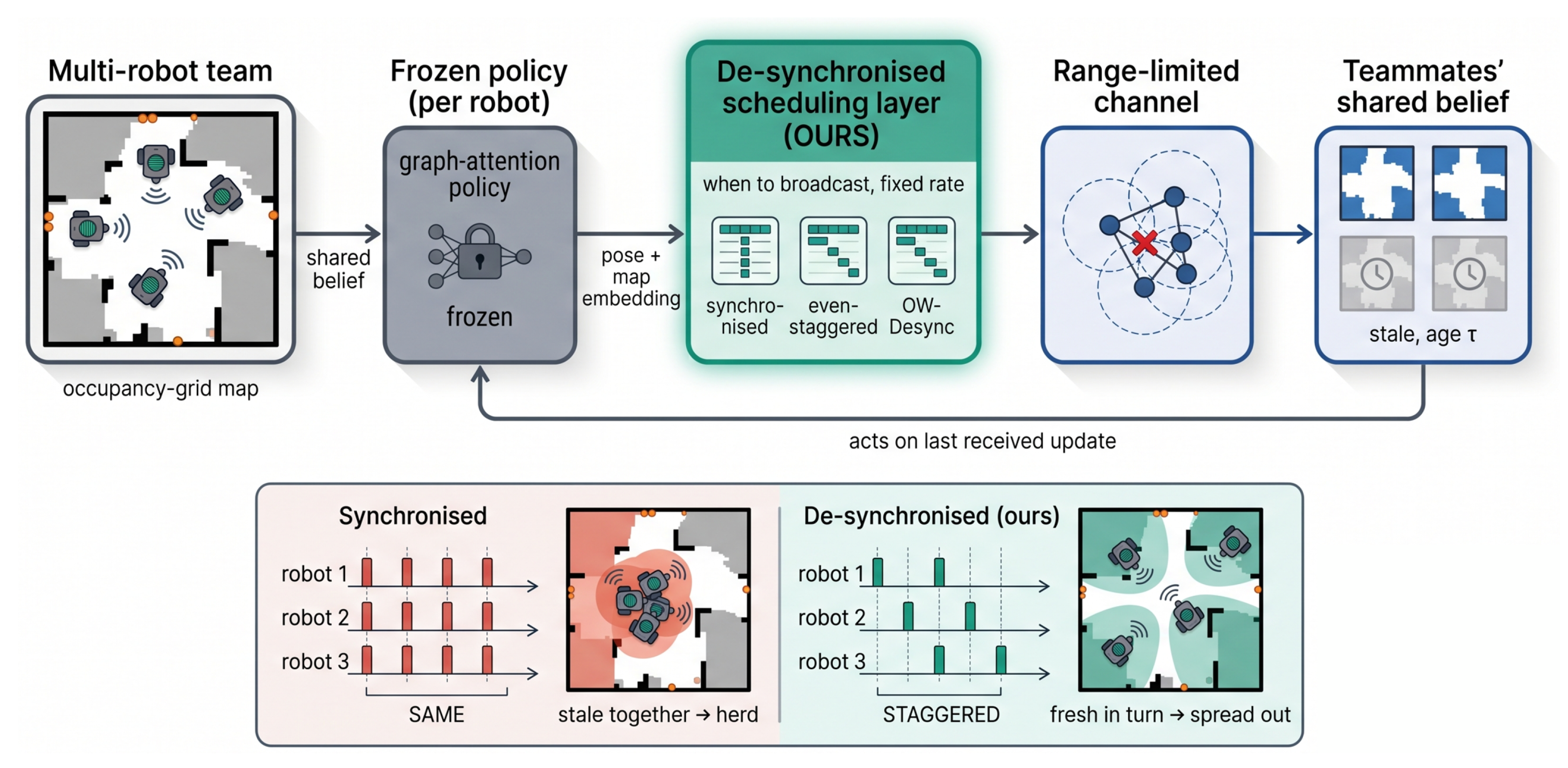
System overview. A frozen, pretrained multi-robot explorer (left) plans against a shared belief of teammates’ poses and map embeddings. We insert a test-time desynchronised scheduling layer that decides, at a fixed per-robot rate, when each robot broadcasts (synchronised, even-staggered, or OW-Desync) over a range-limited, lossy channel; this sets how stale each teammate’s belief is, and hence travel and sensing overlap. Bottom: Broadcasting on a common schedule (left) aligns the robots’ updates, so their beliefs go stale together and they herd onto the same frontiers, whereas desynchronising the phase at the same rate (right) staggers the updates, so the team stays fresh in turn and spreads out. This wasted-effort gap is the synchrony tax.
Figure 1.
System overview. A frozen, pretrained multi-robot explorer (left) plans against a shared belief of teammates’ poses and map embeddings. We insert a test-time desynchronised scheduling layer that decides, at a fixed per-robot rate, when each robot broadcasts (synchronised, even-staggered, or OW-Desync) over a range-limited, lossy channel; this sets how stale each teammate’s belief is, and hence travel and sensing overlap. Bottom: Broadcasting on a common schedule (left) aligns the robots’ updates, so their beliefs go stale together and they herd onto the same frontiers, whereas desynchronising the phase at the same rate (right) staggers the updates, so the team stays fresh in turn and spreads out. This wasted-effort gap is the synchrony tax.
Figure 2.
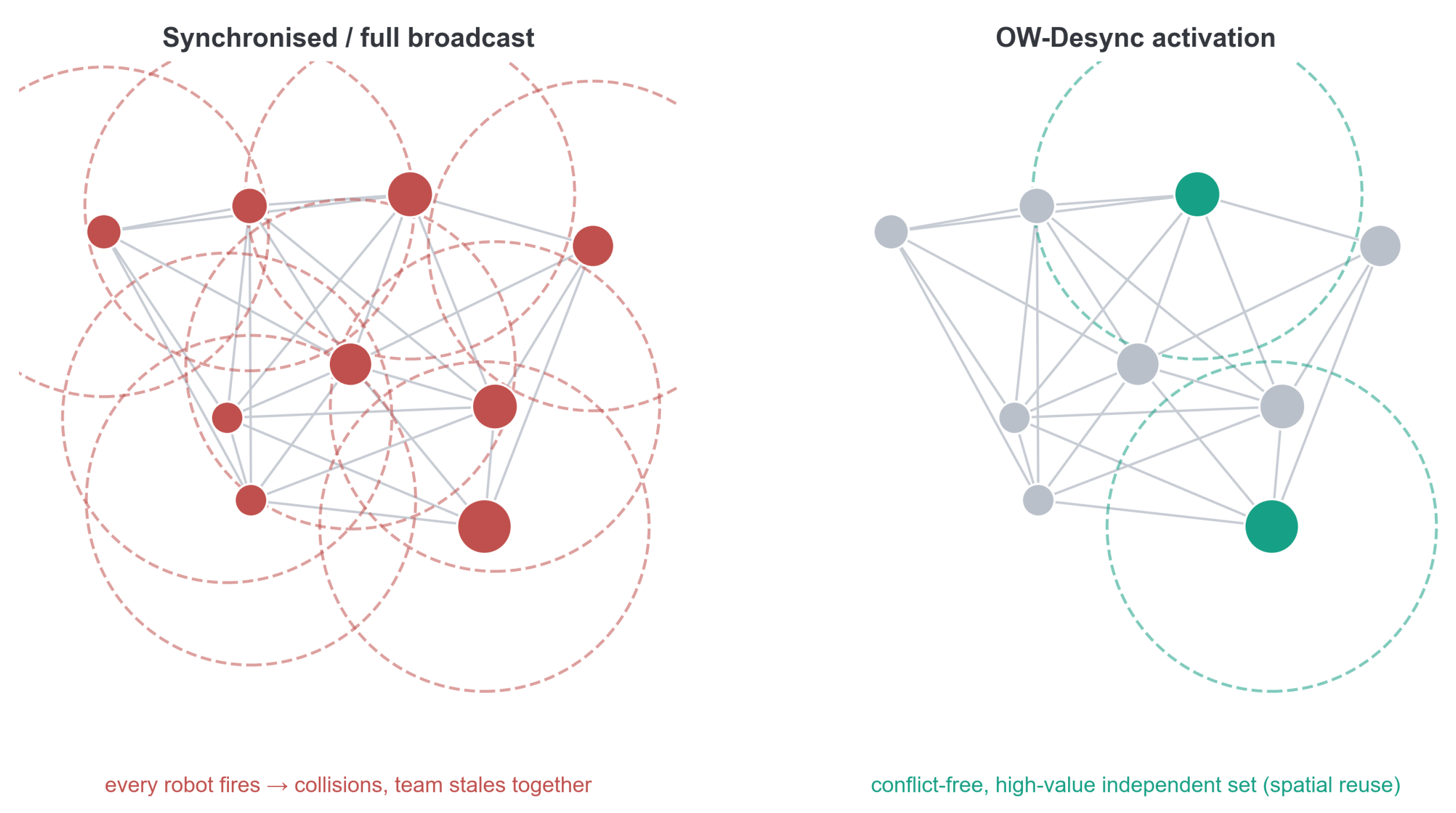
The range-limited interference channel and OW-Desync activation. (Left) Synchronised or full-mesh broadcasting fires every robot in the same slot, so co-located transmitters (dashed range rings) collide and the whole team’s beliefs go stale together. (Right) OW-Desync transmits, each slot, a conflict-free independent set of the interference graph, preferring high-value robots (marker area ∝ weight ), while non-interfering robots reuse the medium spatially. Red nodes denote simultaneous, mutually interfering transmissions; teal nodes form the activated independent set; grey nodes are inactive. Dashed circles show communication/interference range, and solid grey edges join interfering robot pairs. When the graph is complete and robots are symmetric, this reduces exactly to even staggering.
Figure 2.
The range-limited interference channel and OW-Desync activation. (Left) Synchronised or full-mesh broadcasting fires every robot in the same slot, so co-located transmitters (dashed range rings) collide and the whole team’s beliefs go stale together. (Right) OW-Desync transmits, each slot, a conflict-free independent set of the interference graph, preferring high-value robots (marker area ∝ weight ), while non-interfering robots reuse the medium spatially. Red nodes denote simultaneous, mutually interfering transmissions; teal nodes form the activated independent set; grey nodes are inactive. Dashed circles show communication/interference range, and solid grey edges join interfering robot pairs. When the graph is complete and robots are symmetric, this reduces exactly to even staggering.
Figure 3.
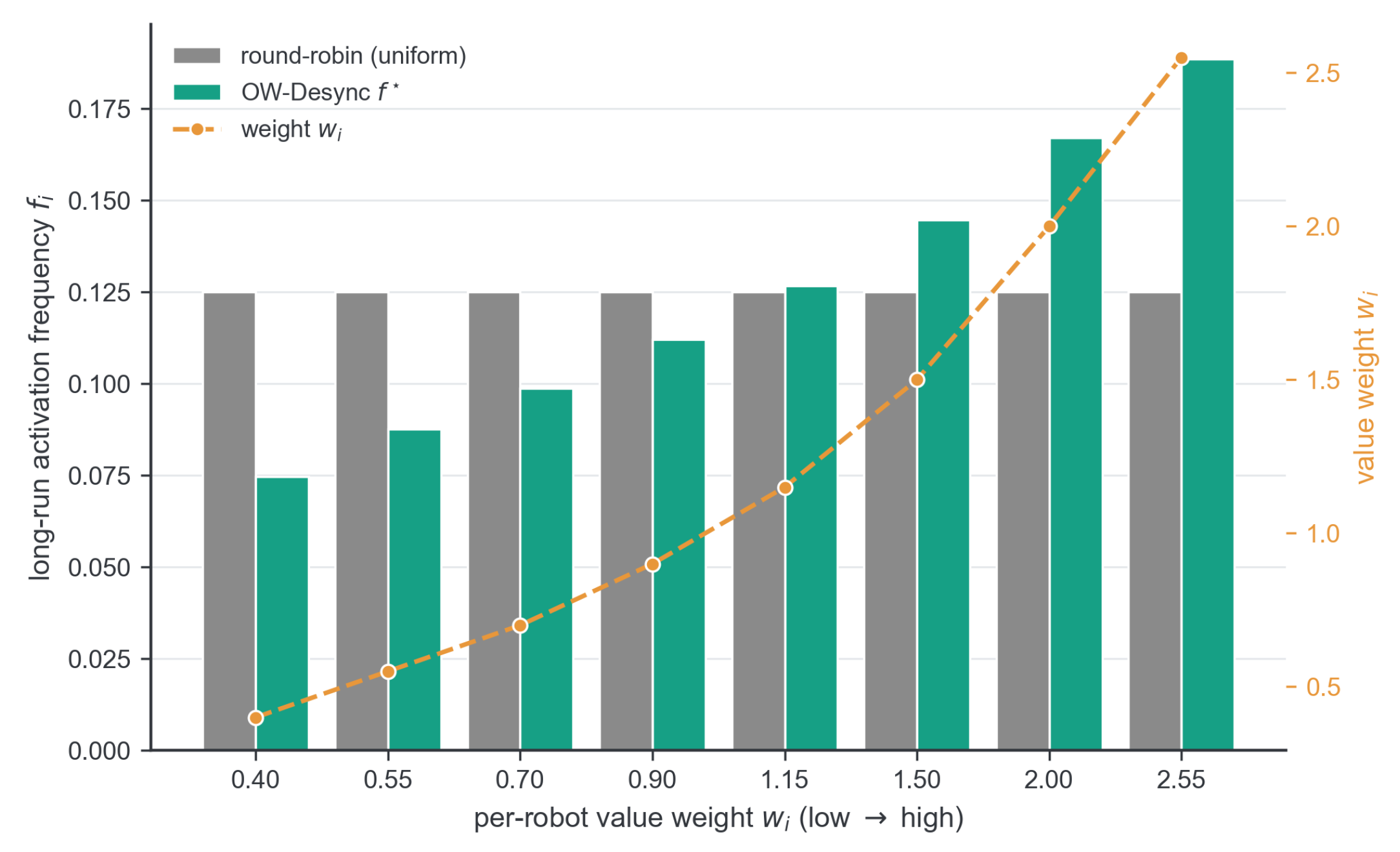
How OW-Desync works in the frequency domain. On a shared medium the convex program assigns each robot a long-run activation frequency (water-filling), giving more airtime to high-value robots (teal) than the uniform round-robin allocation (grey), which lowers the weighted peak Age-of-Information . The reduction grows with weight heterogeneity as shown later in the heterogeneity sweep; when weights are symmetric, is uniform and OW-Desync reduces to even staggering.
Figure 3.
How OW-Desync works in the frequency domain. On a shared medium the convex program assigns each robot a long-run activation frequency (water-filling), giving more airtime to high-value robots (teal) than the uniform round-robin allocation (grey), which lowers the weighted peak Age-of-Information . The reduction grows with weight heterogeneity as shown later in the heterogeneity sweep; when weights are symmetric, is uniform and OW-Desync reduces to even staggering.
Figure 4.
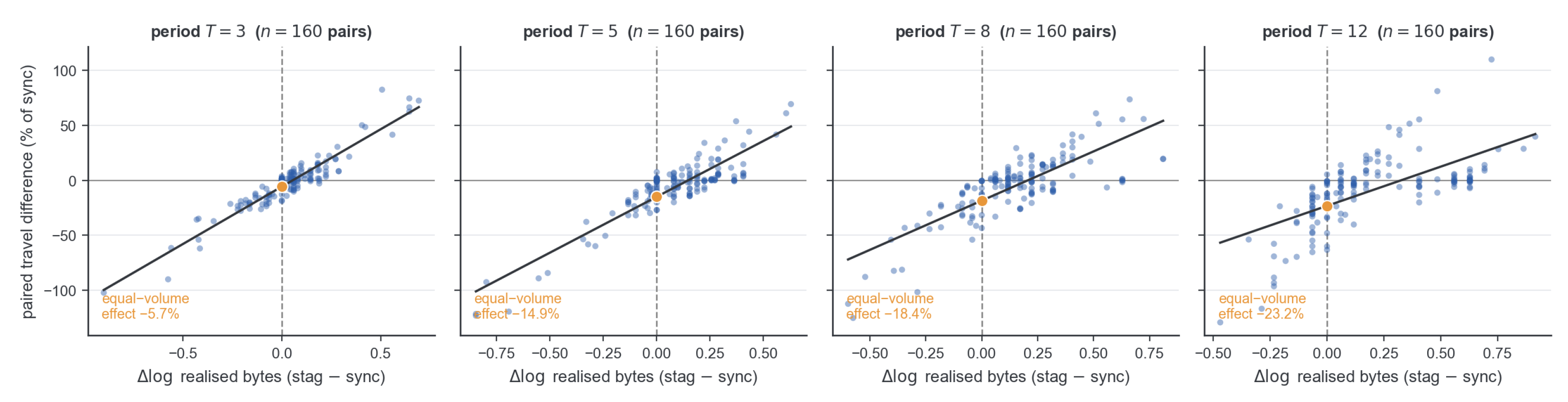
The schedule effect is not a volume effect: each panel plots, for one broadcast period, the paired travel difference (staggered minus synchronised, as % of synchronised travel) against the paired difference in realised log byte volume over matched (map, seed) episodes. Realised bytes co-vary with travel (positive slopes), which is exactly the confound; the regression intercept at equal realised volume ( bytes , orange) remains negative and highly significant at every period ( to , all ), so the desynchronisation gain survives with byte volume held fixed. Grey dashed vertical lines and grey solid horizontal lines mark equal realised volume and zero travel difference, respectively; dark solid lines are least-squares fits, and orange points mark the fitted equal-volume intercepts.
Figure 4.
The schedule effect is not a volume effect: each panel plots, for one broadcast period, the paired travel difference (staggered minus synchronised, as % of synchronised travel) against the paired difference in realised log byte volume over matched (map, seed) episodes. Realised bytes co-vary with travel (positive slopes), which is exactly the confound; the regression intercept at equal realised volume ( bytes , orange) remains negative and highly significant at every period ( to , all ), so the desynchronisation gain survives with byte volume held fixed. Grey dashed vertical lines and grey solid horizontal lines mark equal realised volume and zero travel difference, respectively; dark solid lines are least-squares fits, and orange points mark the fitted equal-volume intercepts.
Figure 5.
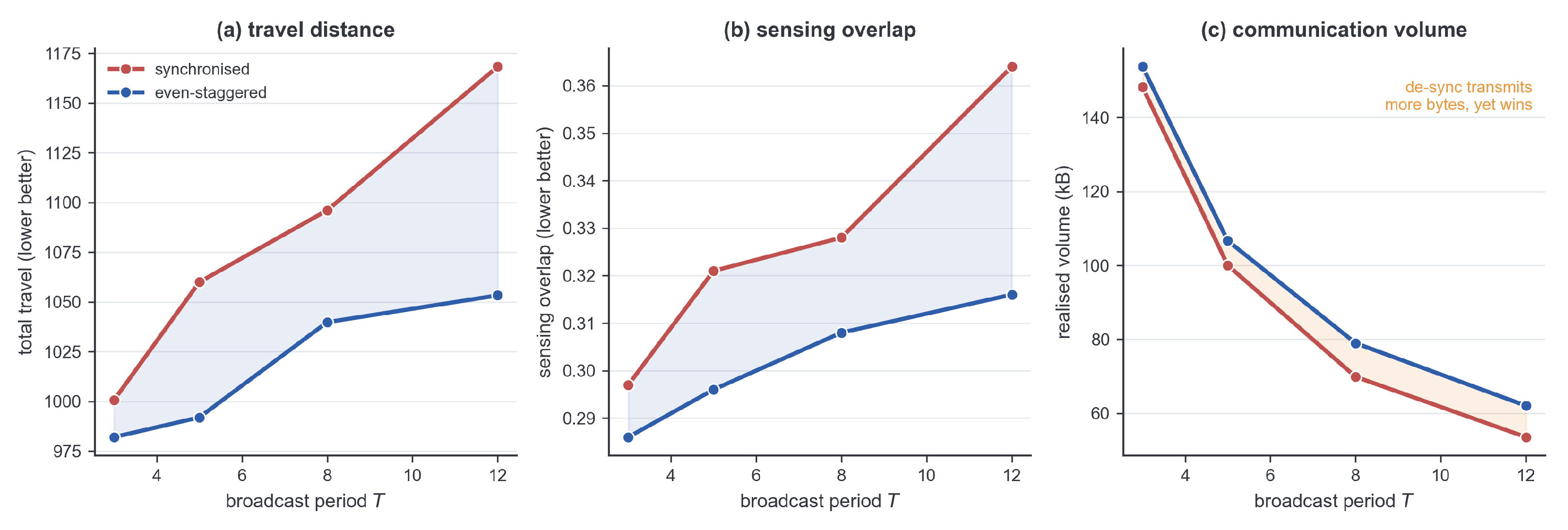
Synchronisation is the controllable cost at a matched per-robot broadcast rate (, periods 3–12). Desynchronised (blue) lies below synchronised (red) in both (a) total travel and (b) sensing overlap, with the largest gap at the scarcest budget; (c) desynchronisation transmits more bytes (up to at period 12) yet travels less, so the gain is timing, not a bandwidth saving. The shaded regions show the between-schedule gap: the blue areas in (a,b) show the efficiency advantage of desynchronisation, and the orange area in (c) shows its additional realised byte volume.
Figure 5.
Synchronisation is the controllable cost at a matched per-robot broadcast rate (, periods 3–12). Desynchronised (blue) lies below synchronised (red) in both (a) total travel and (b) sensing overlap, with the largest gap at the scarcest budget; (c) desynchronisation transmits more bytes (up to at period 12) yet travels less, so the gain is timing, not a bandwidth saving. The shaded regions show the between-schedule gap: the blue areas in (a,b) show the efficiency advantage of desynchronisation, and the orange area in (c) shows its additional realised byte volume.
Figure 6.
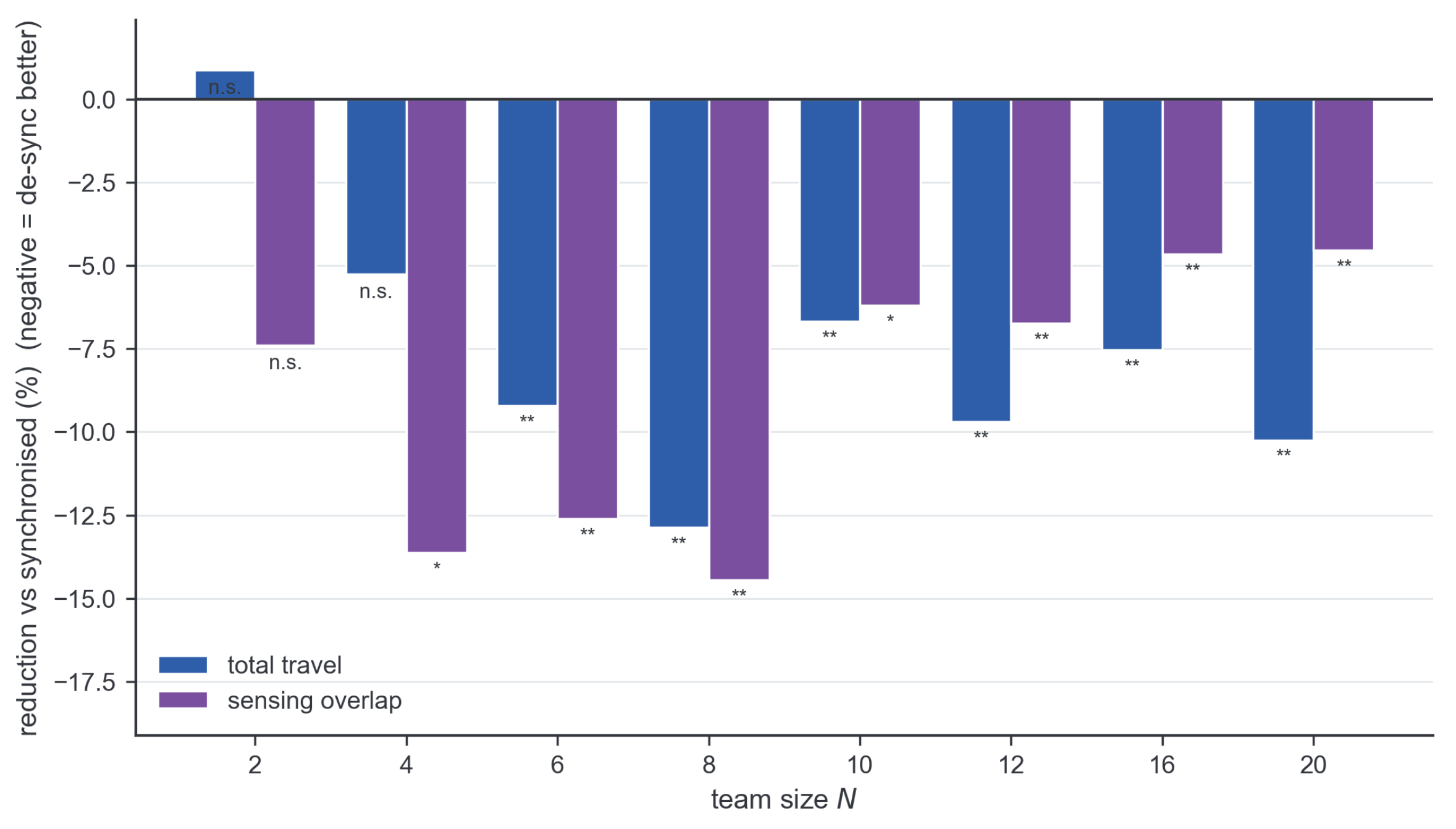
Desynchronisation advantage across team size (–20) from the phase-only control (staggered vs. synchronised periodic at matched budget, interval 12): total-travel (blue) and sensing-overlap (purple) reduction, negative is better. * , ** ; n.s. = not significant.
Figure 6.
Desynchronisation advantage across team size (–20) from the phase-only control (staggered vs. synchronised periodic at matched budget, interval 12): total-travel (blue) and sensing-overlap (purple) reduction, negative is better. * , ** ; n.s. = not significant.
Figure 7.
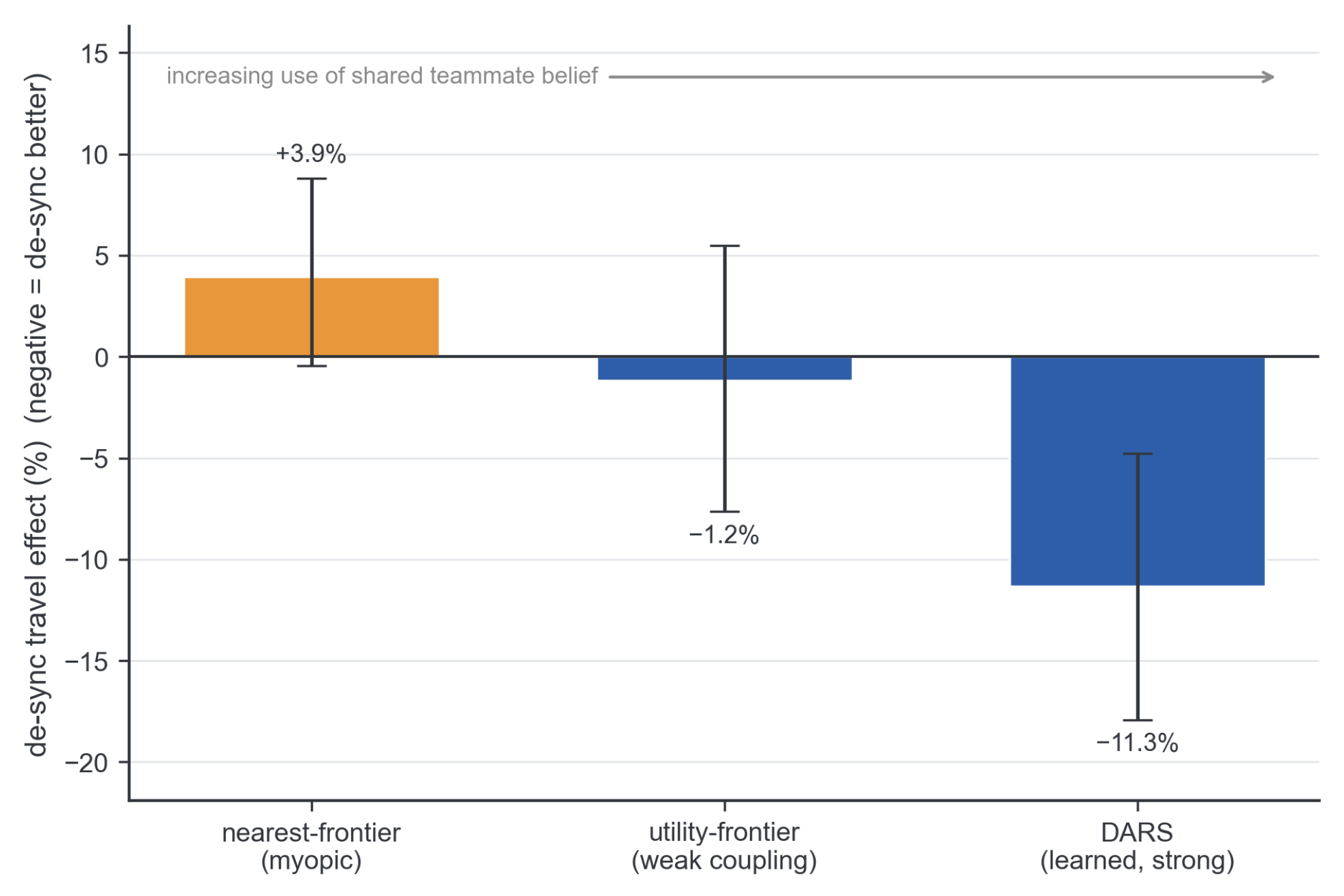
Desynchronisation effect by planner backbone (staggered vs. synchronised periodic, interval 12, ; negative means desynchronisation is better). The benefit grows with how much the planner coordinates through the shared teammate belief: harmful for the myopic nearest-frontier planner, weak for the utility frontier, and strong for the learned graph-attention policy. Error bars are bootstrap confidence intervals (the DARS interval excludes zero; the others do not). The paired Wilcoxon test additionally detects a small but significant harmful effect for nearest-frontier ( travel, ); the bootstrap intervals shown here are wider and are reported separately from those exact p-values, which are given in the text.
Figure 7.
Desynchronisation effect by planner backbone (staggered vs. synchronised periodic, interval 12, ; negative means desynchronisation is better). The benefit grows with how much the planner coordinates through the shared teammate belief: harmful for the myopic nearest-frontier planner, weak for the utility frontier, and strong for the learned graph-attention policy. Error bars are bootstrap confidence intervals (the DARS interval excludes zero; the others do not). The paired Wilcoxon test additionally detects a small but significant harmful effect for nearest-frontier ( travel, ); the bootstrap intervals shown here are wider and are reported separately from those exact p-values, which are given in the text.
Figure 8.
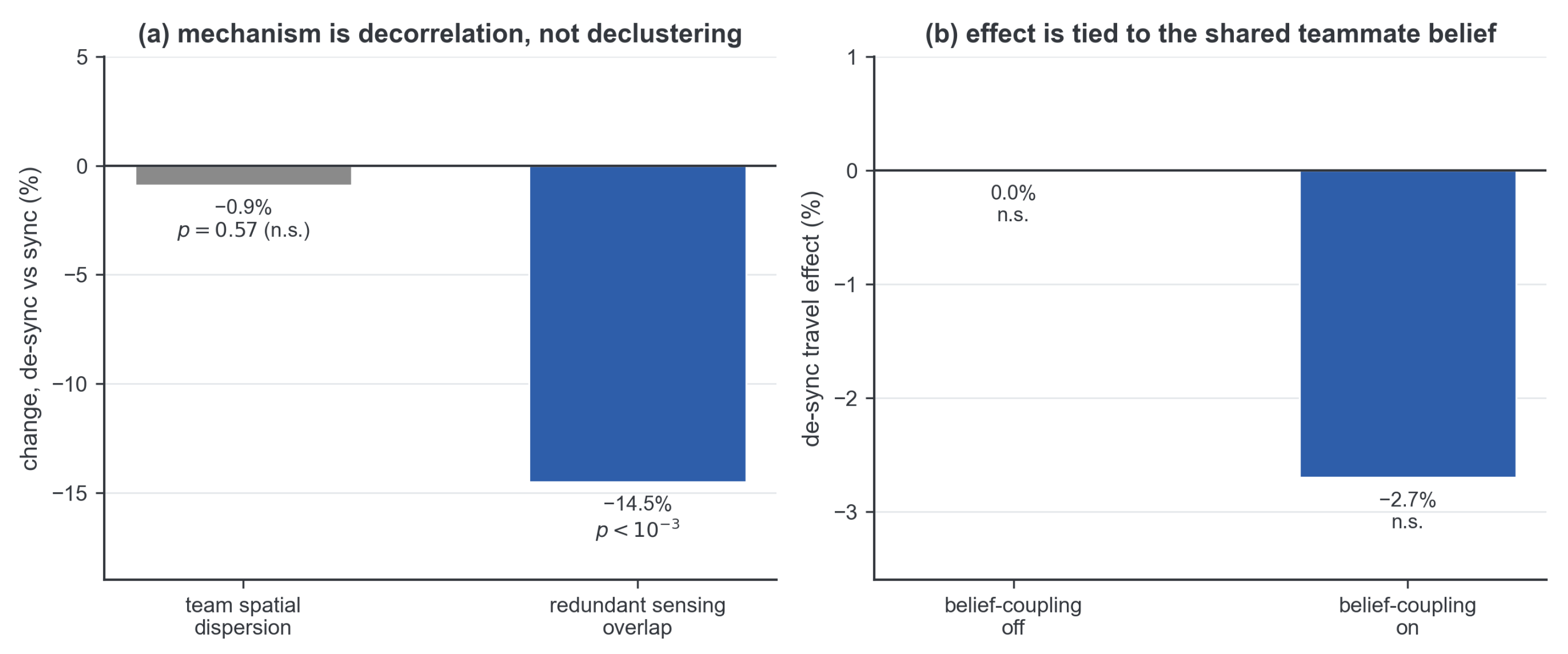
Two controls isolating the mechanism. (a) Desynchronisation leaves team spatial dispersion statistically unchanged (, ) while sharply cutting redundant sensing overlap (, ): the gain comes from decorrelating stale beliefs, not from physically spreading the robots. (b) When the planner is made to ignore the shared teammate belief (deconfliction weight set to zero) the desynchronisation effect vanishes exactly (); restoring belief coupling restores it only directionally (, n.s.), so the causal force rests on the exact null at zero coupling. n.s. means not significant.
Figure 8.
Two controls isolating the mechanism. (a) Desynchronisation leaves team spatial dispersion statistically unchanged (, ) while sharply cutting redundant sensing overlap (, ): the gain comes from decorrelating stale beliefs, not from physically spreading the robots. (b) When the planner is made to ignore the shared teammate belief (deconfliction weight set to zero) the desynchronisation effect vanishes exactly (); restoring belief coupling restores it only directionally (, n.s.), so the causal force rests on the exact null at zero coupling. n.s. means not significant.
Figure 9.
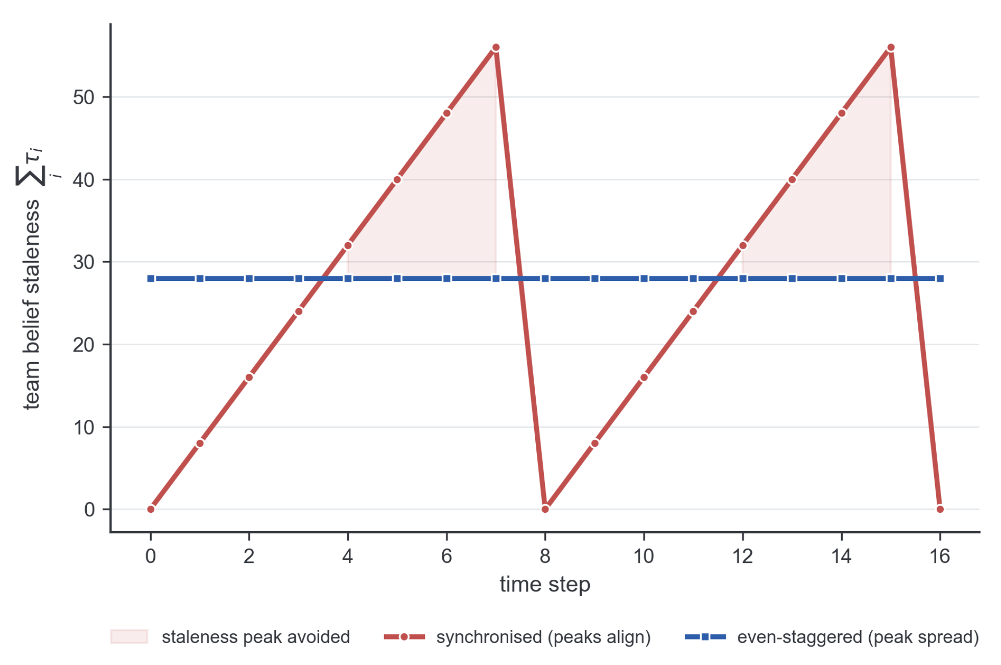
Time-domain view of the mechanism (, period ). Each link’s staleness is a sawtooth; under synchronised broadcasting the sawtooths peak together so the team-staleness sum swings to a large peak (red), whereas even staggering spreads the offsets and flattens the sum toward its (identical) time mean (blue). The shaded area is the peak the staleness-to-overlap bound penalises and that Proposition 3 minimises.
Figure 9.
Time-domain view of the mechanism (, period ). Each link’s staleness is a sawtooth; under synchronised broadcasting the sawtooths peak together so the team-staleness sum swings to a large peak (red), whereas even staggering spreads the offsets and flattens the sum toward its (identical) time mean (blue). The shaded area is the peak the staleness-to-overlap bound penalises and that Proposition 3 minimises.
Figure 10.
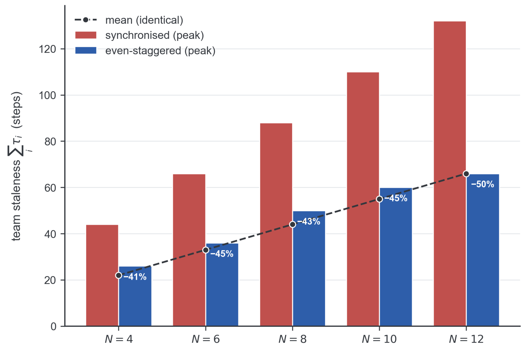
Desynchronisation decorrelates staleness at constant mean. For broadcast period the team-staleness sum has identical time mean (dashed) under synchronised and staggered schedules, but even staggering roughly halves its peak (percentages shown), the quantity the staleness-to-overlap bound penalises.
Figure 10.
Desynchronisation decorrelates staleness at constant mean. For broadcast period the team-staleness sum has identical time mean (dashed) under synchronised and staggered schedules, but even staggering roughly halves its peak (percentages shown), the quantity the staleness-to-overlap bound penalises.
Figure 11.
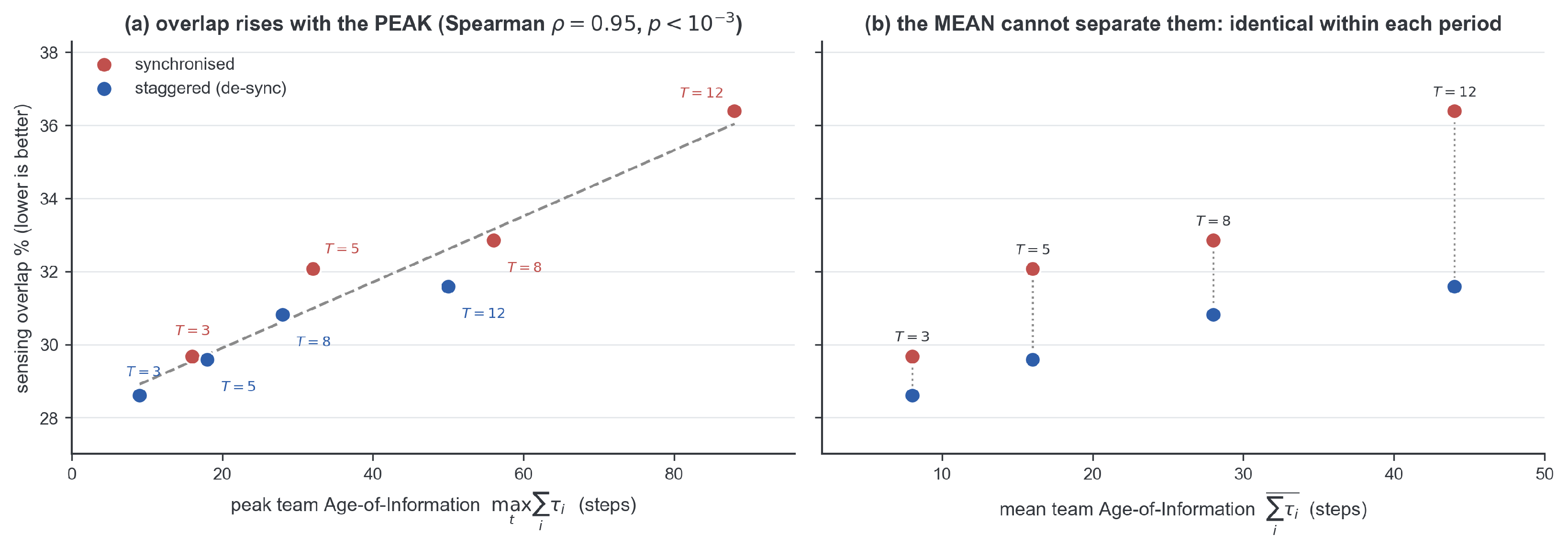
Empirical support for Proposition 2 in the Age-of-Information metric. Each point is one of eight broadcast conditions (synchronised and staggered periodic, intervals ). (a) Measured sensing overlap rises with the team’s peak Age-of-Information, the peak of the team-staleness sum (Spearman , ); synchronised schedules occupy the high-AoI end and staggered schedules the low end. (b) The same overlap values plotted against the mean of the team-staleness sum: within each period the two schedules share one mean by construction (dotted verticals), yet their overlaps differ, so the mean cannot explain the separation of the peak.
Figure 11.
Empirical support for Proposition 2 in the Age-of-Information metric. Each point is one of eight broadcast conditions (synchronised and staggered periodic, intervals ). (a) Measured sensing overlap rises with the team’s peak Age-of-Information, the peak of the team-staleness sum (Spearman , ); synchronised schedules occupy the high-AoI end and staggered schedules the low end. (b) The same overlap values plotted against the mean of the team-staleness sum: within each period the two schedules share one mean by construction (dotted verticals), yet their overlaps differ, so the mean cannot explain the separation of the peak.
Figure 12.
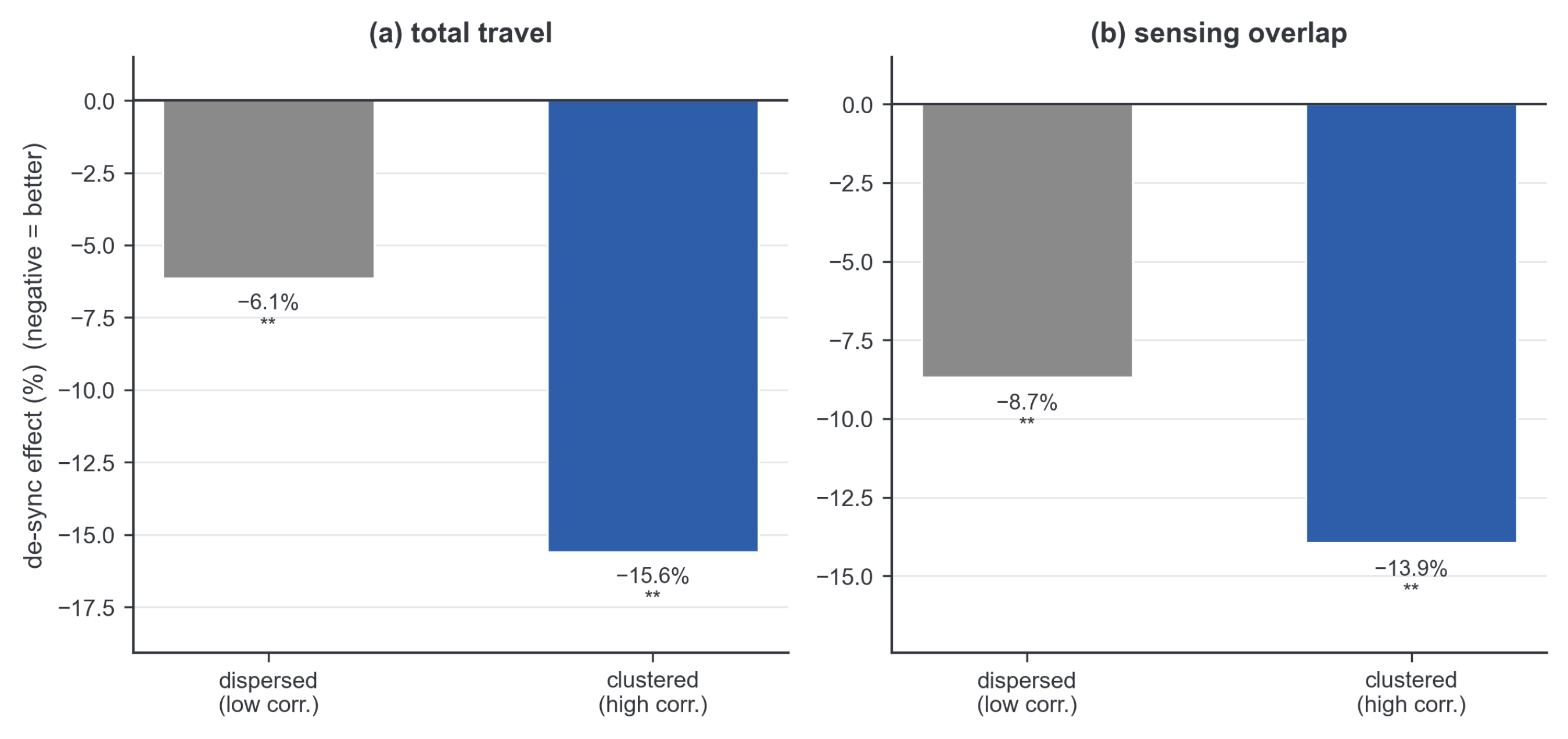
The desynchronisation benefit grows with the team’s initial information correlation, as predicted by [
44]. Both (
a) total travel and (
b) sensing overlap improve more for clustered, high-correlation spawns (
,
) than for dispersed, low-correlation ones (
,
) (
, interval 12, staggered vs. synchronised periodic; **
). More correlated sources gain more from desynchronisation.
Figure 12.
The desynchronisation benefit grows with the team’s initial information correlation, as predicted by [
44]. Both (
a) total travel and (
b) sensing overlap improve more for clustered, high-correlation spawns (
,
) than for dispersed, low-correlation ones (
,
) (
, interval 12, staggered vs. synchronised periodic; **
). More correlated sources gain more from desynchronisation.
Figure 13.
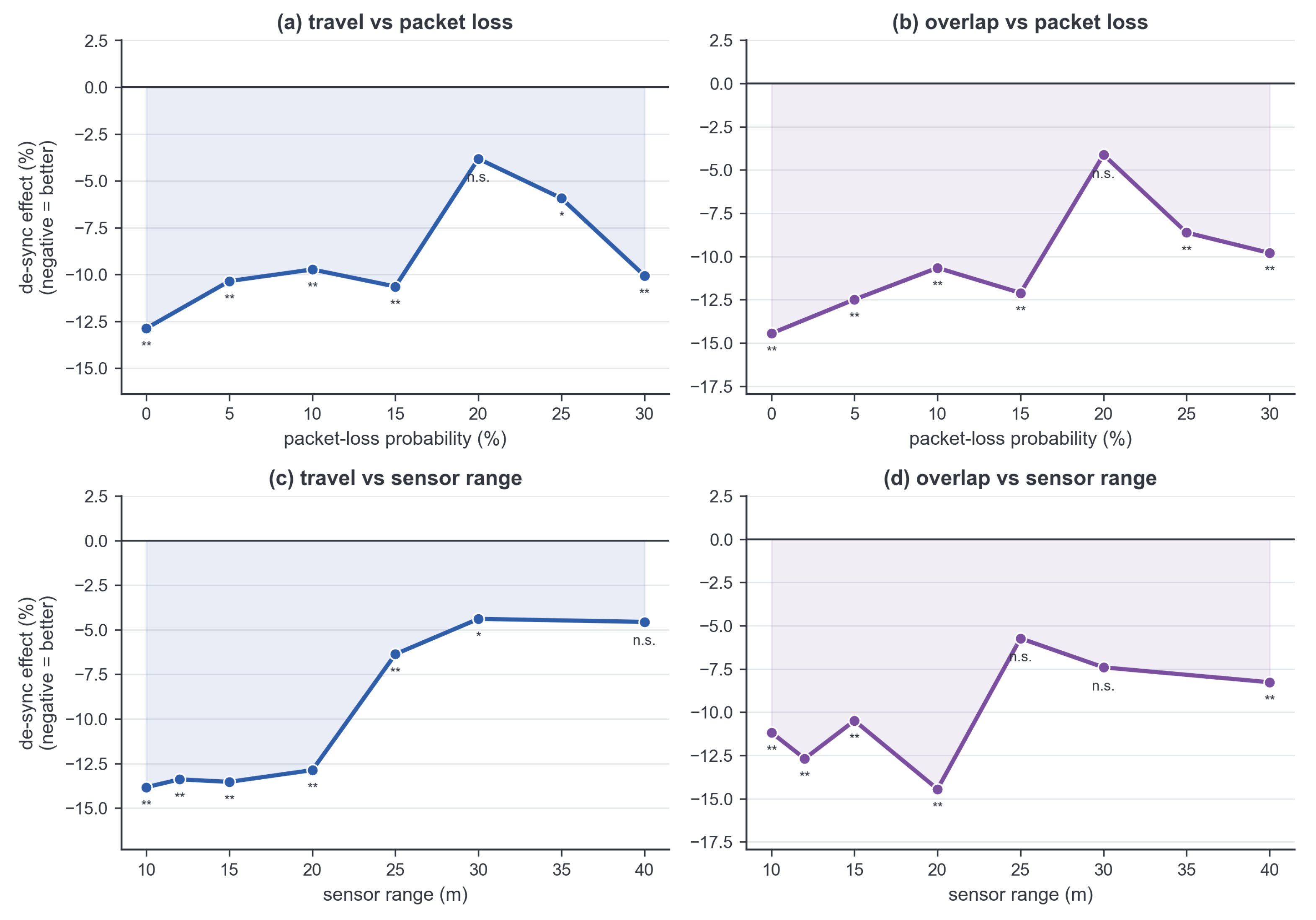
Desynchronisation benefit across two stressors at , interval 12 (staggered vs. synchronised periodic; per point). (a,b) Travel and sensing overlap across seven packet-loss levels (0–): the gain persists, the lone shallow point at being consistent with sampling variation flanked by significant neighbours. (c,d) Travel and overlap across seven sensor ranges (10–40 m): the gain holds across the sweep (the 40 m point marginal, ) and grows at shorter range, where robots rely more on the shared belief. Shaded areas between each curve and zero visualise the magnitude and direction of the schedule effect. * , ** ; n.s. means not significant.
Figure 13.
Desynchronisation benefit across two stressors at , interval 12 (staggered vs. synchronised periodic; per point). (a,b) Travel and sensing overlap across seven packet-loss levels (0–): the gain persists, the lone shallow point at being consistent with sampling variation flanked by significant neighbours. (c,d) Travel and overlap across seven sensor ranges (10–40 m): the gain holds across the sweep (the 40 m point marginal, ) and grows at shorter range, where robots rely more on the shared belief. Shaded areas between each curve and zero visualise the magnitude and direction of the schedule effect. * , ** ; n.s. means not significant.
Figure 14.
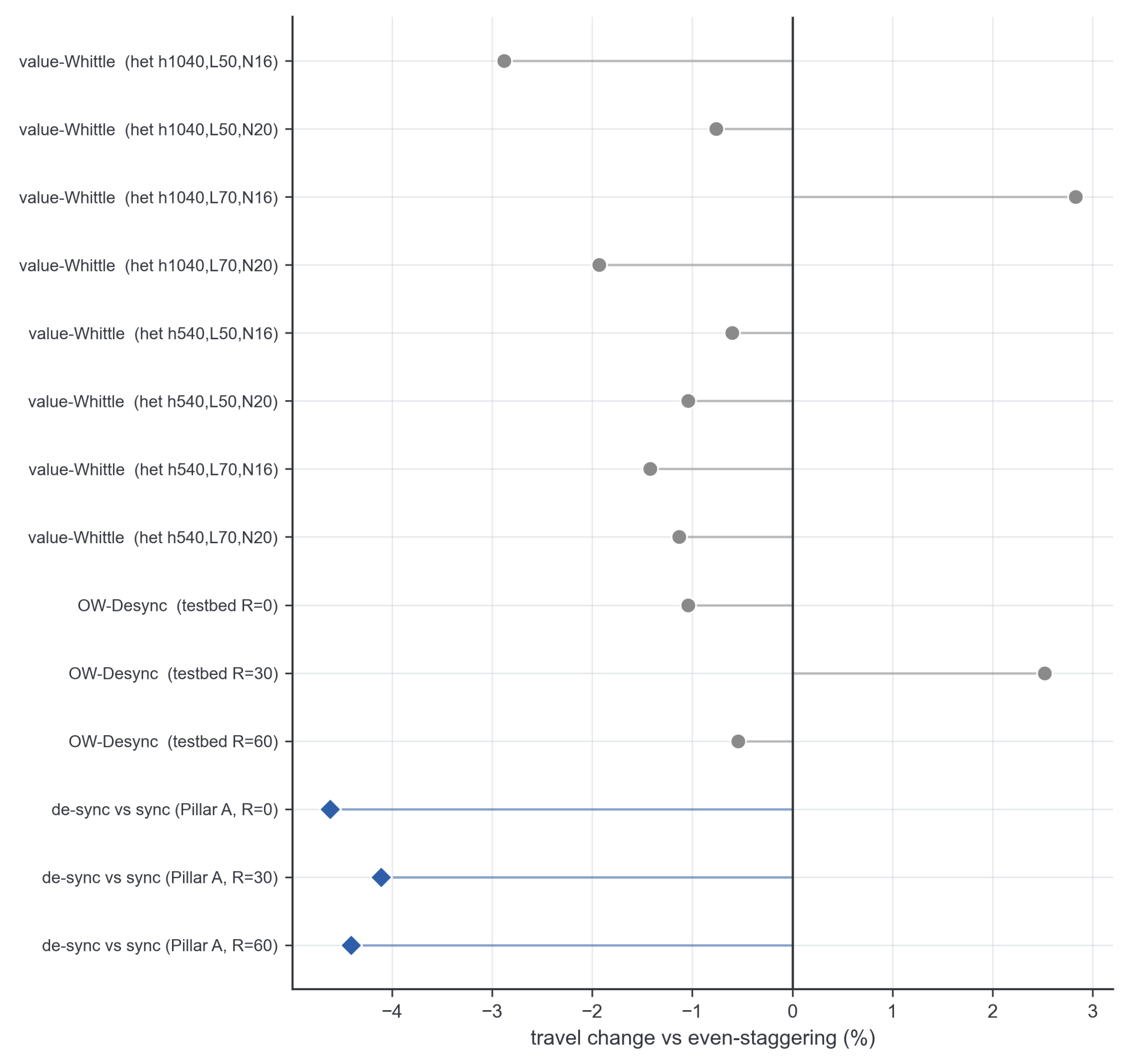
Effect sizes on the exploration objective, measured as travel change relative to even staggering (negative is better). The value/loss-aware Whittle scheduler across heterogeneity and loss regimes, and OW-Desync on the testbed, all cluster around zero (grey; none significantly beats even staggering), whereas the desynchronised-vs-synchronised contrast (blue diamonds) moves travel by to . On this objective, scheduling identity is near-optimal; only whether the team is synchronised matters.
Figure 14.
Effect sizes on the exploration objective, measured as travel change relative to even staggering (negative is better). The value/loss-aware Whittle scheduler across heterogeneity and loss regimes, and OW-Desync on the testbed, all cluster around zero (grey; none significantly beats even staggering), whereas the desynchronised-vs-synchronised contrast (blue diamonds) moves travel by to . On this objective, scheduling identity is near-optimal; only whether the team is synchronised matters.
Figure 15.
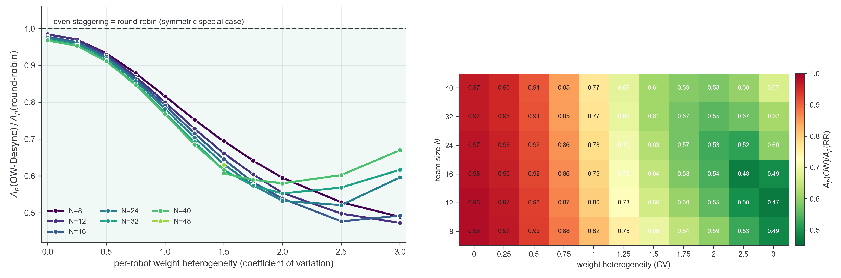
OW-Desync weighted peak-AoI relative to round-robin at matched budget on the interference graph. (Left) The ratio is close to 1 (–) at zero weight heterogeneity on this range-limited graph (Corollary 1 predicts exact coincidence on a symmetric shared medium) and falls as per-robot weight heterogeneity grows up to , with a partial rebound for the largest teams beyond, for team sizes –48. (Right) The same gain as a heatmap over team size and heterogeneity, where every cell with improves on average (greener is a larger OW-Desync advantage). The gain is on the communication-freshness objective OW-Desync provably optimises.
Figure 15.
OW-Desync weighted peak-AoI relative to round-robin at matched budget on the interference graph. (Left) The ratio is close to 1 (–) at zero weight heterogeneity on this range-limited graph (Corollary 1 predicts exact coincidence on a symmetric shared medium) and falls as per-robot weight heterogeneity grows up to , with a partial rebound for the largest teams beyond, for team sizes –48. (Right) The same gain as a heatmap over team size and heterogeneity, where every cell with improves on average (greener is a larger OW-Desync advantage). The gain is on the communication-freshness objective OW-Desync provably optimises.
Figure 16.
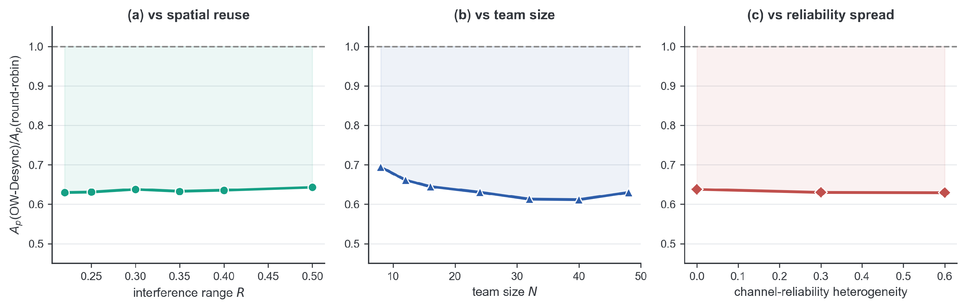
The OW-Desync weighted peak-AoI gain (ratio to round-robin at matched budget; lower is better, dashed line is parity) stays well below 1 across (a) interference range/spatial reuse, (b) team size –48, and (c) heterogeneous channel reliability, so the advantage is not an artefact of any single operating point. The shaded area between each curve and the parity line visualises the magnitude of the OW-Desync advantage.
Figure 16.
The OW-Desync weighted peak-AoI gain (ratio to round-robin at matched budget; lower is better, dashed line is parity) stays well below 1 across (a) interference range/spatial reuse, (b) team size –48, and (c) heterogeneous channel reliability, so the advantage is not an artefact of any single operating point. The shaded area between each curve and the parity line visualises the magnitude of the OW-Desync advantage.
Figure 17.
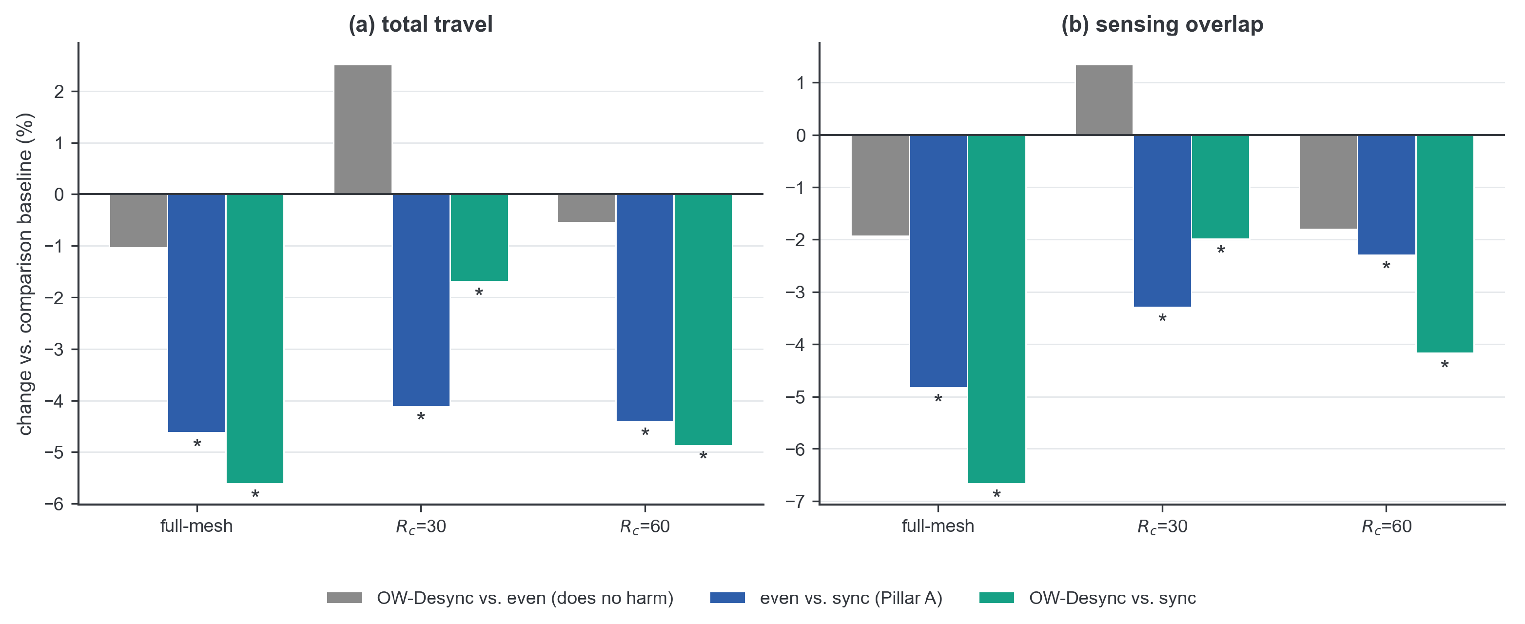
On the frozen explorer under a range-limited channel (, heterogeneous sensing, paired over 240 map–seed pairs per cell). OW-Desync ties even staggering on travel at every communication range (grey, all not significant), while both desynchronised schedules retain a significant advantage over synchronised broadcasting (blue, green; * marks ), confirming that the synchrony-tax benefit persists on the interference-limited channel.
Figure 17.
On the frozen explorer under a range-limited channel (, heterogeneous sensing, paired over 240 map–seed pairs per cell). OW-Desync ties even staggering on travel at every communication range (grey, all not significant), while both desynchronised schedules retain a significant advantage over synchronised broadcasting (blue, green; * marks ), confirming that the synchrony-tax benefit persists on the interference-limited channel.
Figure 18.
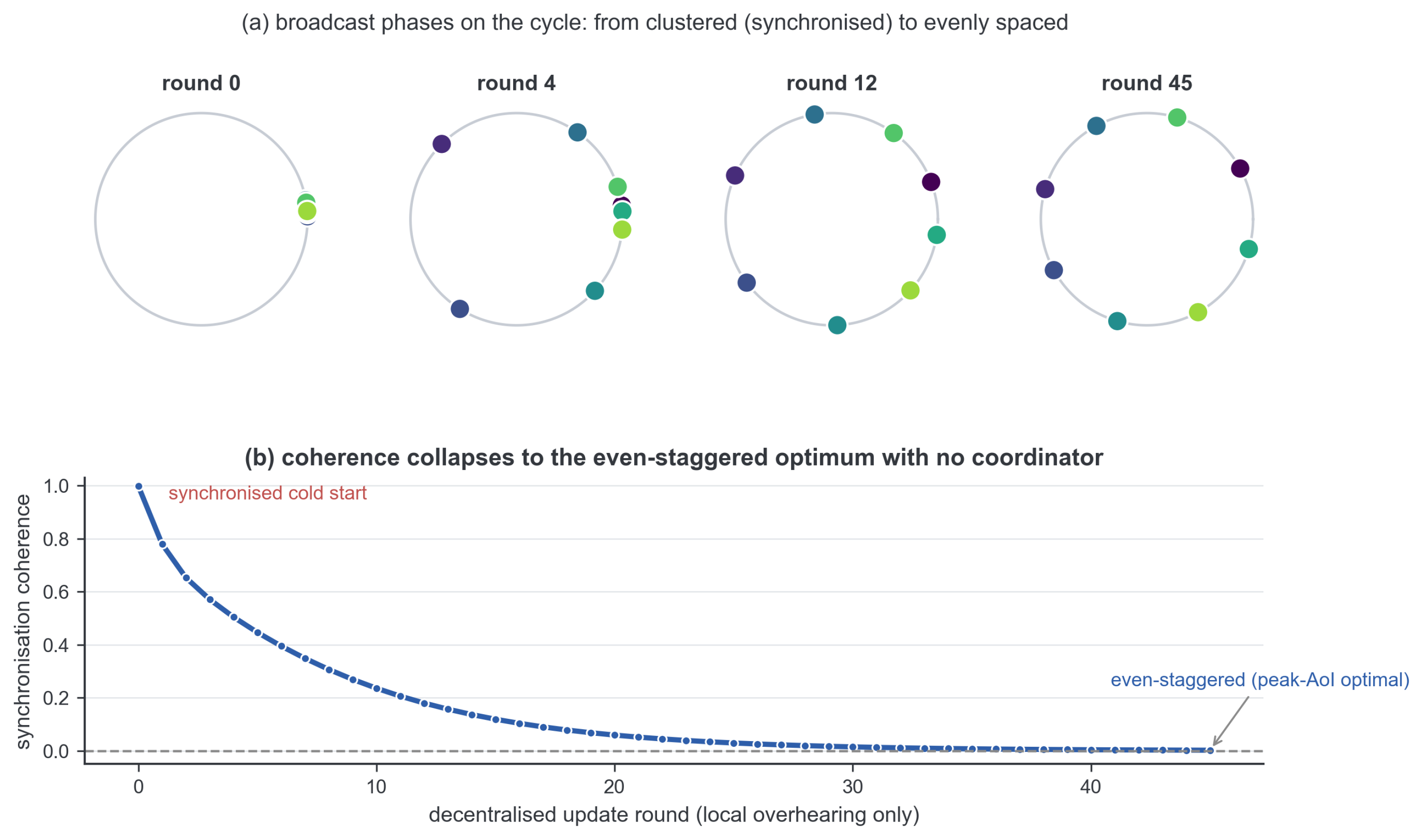
The even-staggered schedule is reachable with no coordinator. Starting from a fully synchronised cold start, a decentralised desynchronisation primitive in which each robot nudges its broadcast phase away from the neighbours it overhears (a) drives the phases to even spacing on the broadcast cycle and (b) collapses the synchronisation coherence to the even-staggered, peak-AoI-optimal configuration, using only local overhearing (). In (a), the eight colours identify the eight robots; in (b), the blue curve is synchronisation coherence and the grey dashed line marks the even-staggered optimum.
Figure 18.
The even-staggered schedule is reachable with no coordinator. Starting from a fully synchronised cold start, a decentralised desynchronisation primitive in which each robot nudges its broadcast phase away from the neighbours it overhears (a) drives the phases to even spacing on the broadcast cycle and (b) collapses the synchronisation coherence to the even-staggered, peak-AoI-optimal configuration, using only local overhearing (). In (a), the eight colours identify the eight robots; in (b), the blue curve is synchronisation coherence and the grey dashed line marks the even-staggered optimum.
Figure 19.
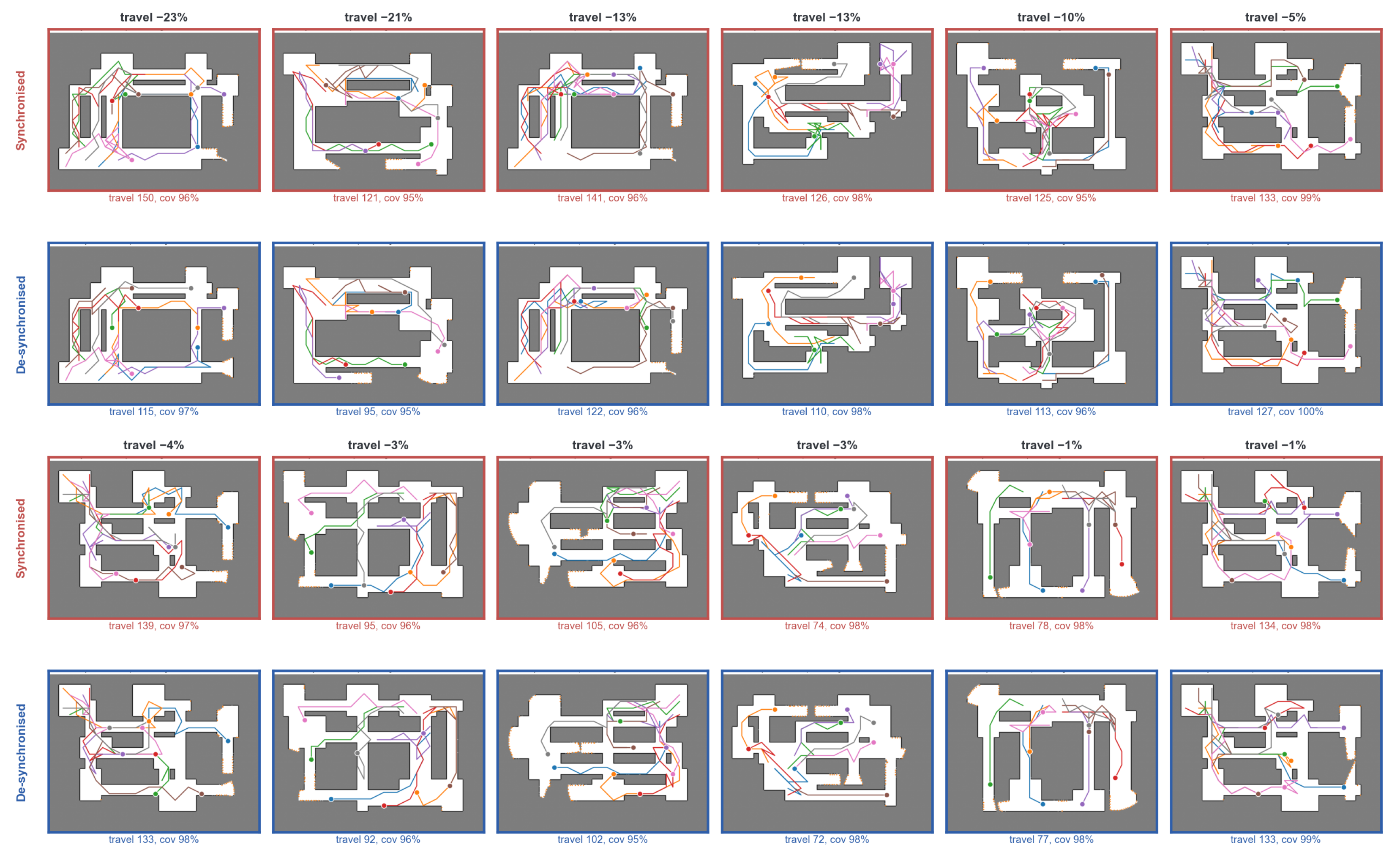
Synchronised (rows 1 and 3, red) vs. desynchronised/even-staggered (rows 2 and 4, blue) exploration at matched bandwidth (, broadcast period ); coloured curves are the eight robot trajectories, and the grey/white background is the occupancy map. Desynchronisation cuts herding and redundant travel; each column is one episode (a map and start-layout seed), ordered by the travel reduction printed above each column ( to ); all reduce travel at essentially unchanged coverage (within percentage points, equal or higher in 8 of 12), selected from a 20-map -seed sweep to illustrate the mechanism; aggregate statistics over all maps and seeds are reported above.
Figure 19.
Synchronised (rows 1 and 3, red) vs. desynchronised/even-staggered (rows 2 and 4, blue) exploration at matched bandwidth (, broadcast period ); coloured curves are the eight robot trajectories, and the grey/white background is the occupancy map. Desynchronisation cuts herding and redundant travel; each column is one episode (a map and start-layout seed), ordered by the travel reduction printed above each column ( to ); all reduce travel at essentially unchanged coverage (within percentage points, equal or higher in 8 of 12), selected from a 20-map -seed sweep to illustrate the mechanism; aggregate statistics over all maps and seeds are reported above.
Figure 20.
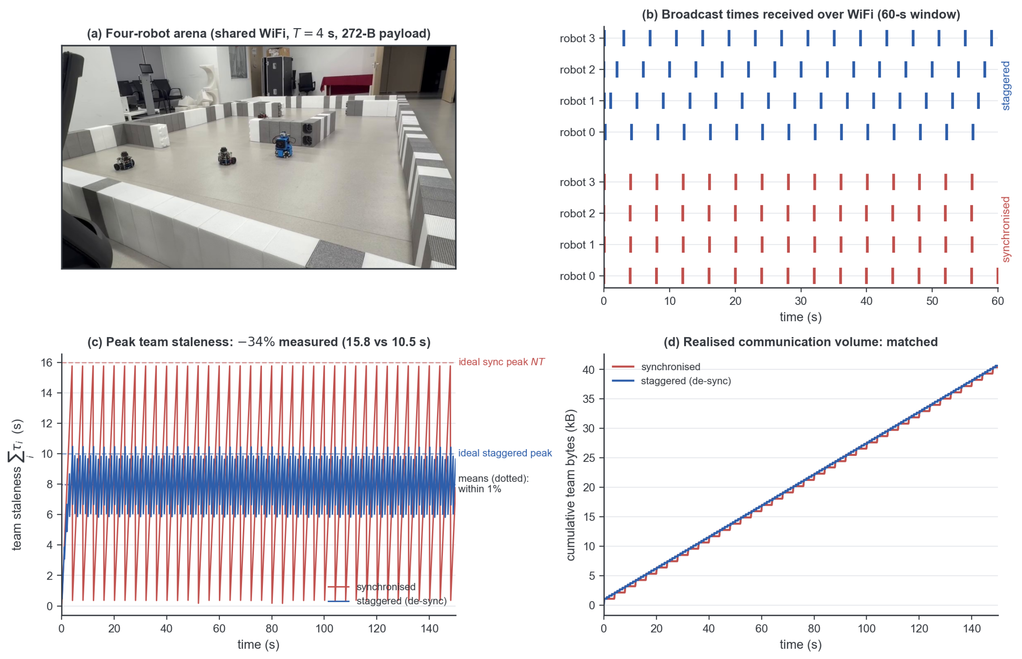
Hardware demonstration of the synchrony-tax mechanism (four robots, real WiFi, one paired trial per condition). (a) The walled arena with the four-robot team. (b) Broadcast times as received at the central monitor: synchronised (red) robots fire in lockstep; staggered (blue) robots realise even offsets one second apart. (c) Team staleness : synchronisation drives the peak to the worst case while staggering holds it near the no-jitter staggered optimum (dashed), the worst-case-versus-optimum ordering that Proposition 3 formalises; the means (dotted) agree to within , so the difference is purely in the peak. (d) Cumulative team communication volume: the two schedules transmit at the same rate with identical payloads, so the curves coincide and the staleness gap is attributable to timing alone.
Figure 20.
Hardware demonstration of the synchrony-tax mechanism (four robots, real WiFi, one paired trial per condition). (a) The walled arena with the four-robot team. (b) Broadcast times as received at the central monitor: synchronised (red) robots fire in lockstep; staggered (blue) robots realise even offsets one second apart. (c) Team staleness : synchronisation drives the peak to the worst case while staggering holds it near the no-jitter staggered optimum (dashed), the worst-case-versus-optimum ordering that Proposition 3 formalises; the means (dotted) agree to within , so the difference is purely in the peak. (d) Cumulative team communication volume: the two schedules transmit at the same rate with identical payloads, so the curves coincide and the staleness gap is attributable to timing alone.
Figure 21.
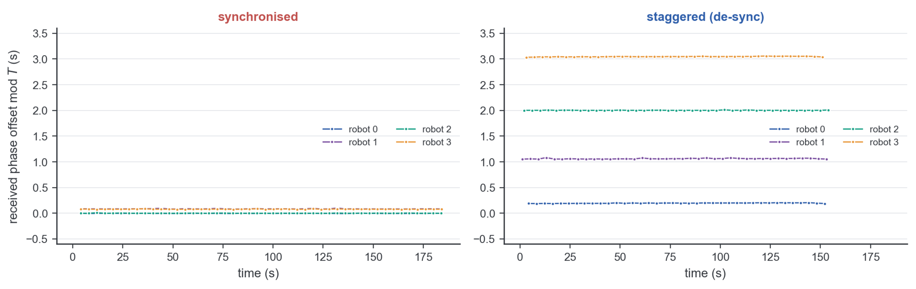
Long-run stability of the hardware schedules: received phase offsets (mod
T) of every broadcast over the full recordings. The synchronised robots stay aligned (
left) and the staggered robots hold their assigned offsets (
right) throughout, with per-robot drift below 5 ms per minute and offset bands within
ms, so asynchronous execution and WiFi jitter did not re-align the schedules over the mission; longer deployments can re-apply the decentralised primitive of
Figure 18 online.
Figure 21.
Long-run stability of the hardware schedules: received phase offsets (mod
T) of every broadcast over the full recordings. The synchronised robots stay aligned (
left) and the staggered robots hold their assigned offsets (
right) throughout, with per-robot drift below 5 ms per minute and offset bands within
ms, so asynchronous execution and WiFi jitter did not re-align the schedules over the mission; longer deployments can re-apply the decentralised primitive of
Figure 18 online.
Figure 22.
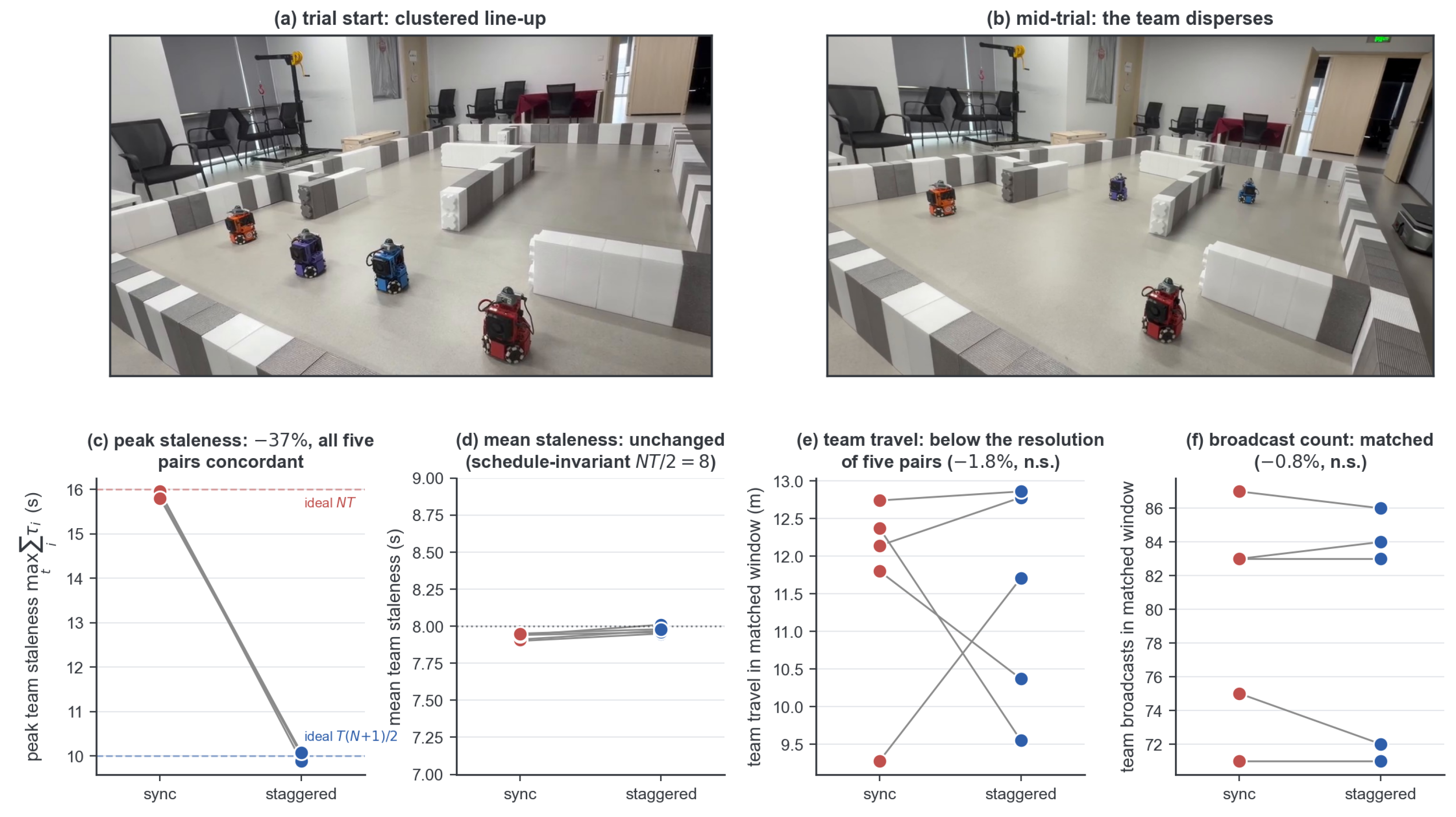
Five repeated paired hardware trials on the second fleet (matched analysis windows). (a) Trial start: the four robots begin in a clustered line-up. (b) Mid-trial: the team disperses through the arena. (c) Peak team staleness: all five pairs fall from the synchronised worst case to the staggered optimum (; dashed lines are the no-jitter ideals and ). (d) Mean team staleness: within s of the schedule-invariant s in every run. (e) Team travel over the matched window: below the resolution of five pairs (, n.s.; the simulation-scale effect needs roughly twenty pairs). (f) Broadcast counts: the matched-rate control holds (, n.s.).
Figure 22.
Five repeated paired hardware trials on the second fleet (matched analysis windows). (a) Trial start: the four robots begin in a clustered line-up. (b) Mid-trial: the team disperses through the arena. (c) Peak team staleness: all five pairs fall from the synchronised worst case to the staggered optimum (; dashed lines are the no-jitter ideals and ). (d) Mean team staleness: within s of the schedule-invariant s in every run. (e) Team travel over the matched window: below the resolution of five pairs (, n.s.; the simulation-scale effect needs roughly twenty pairs). (f) Broadcast counts: the matched-rate control holds (, n.s.).
Table 1.
Broadcast schedulers at a matched scarce budget (, ≈47–50 kB communication). Coverage and communication are matched; the desynchronised and event-triggered schedules cut travel and overlap. Lower travel/overlap/steps are better.
Table 1.
Broadcast schedulers at a matched scarce budget (, ≈47–50 kB communication). Coverage and communication are matched; the desynchronised and event-triggered schedules cut travel and overlap. Lower travel/overlap/steps are better.
| Scheduler | Coverage | Comm (103 B) | Travel | Overlap | Steps |
|---|
| Periodic (synchronised) | 0.966 | 47 | 1231.2 | 0.378 | 17.7 |
| Random (desynchronised) | 0.966 | 48 | 1101.2 | 0.337 | 15.8 |
| Event-triggered | 0.966 | 50 | 1124.1 | 0.340 | 16.2 |
Table 2.
Staggered vs. synchronised periodic at matched per-robot broadcast rate (, paired episodes per period; negative = de-sync better; paired Wilcoxon). The last column gives the Holm-adjusted travel p across the three-period sweep; every period stays significant (), including the marginal period 8. The realised byte volume is not held equal: staggered transmits up to more (column 2), yet travels and overlaps less, so the gain is not a bandwidth saving.
Table 2.
Staggered vs. synchronised periodic at matched per-robot broadcast rate (, paired episodes per period; negative = de-sync better; paired Wilcoxon). The last column gives the Holm-adjusted travel p across the three-period sweep; every period stays significant (), including the marginal period 8. The realised byte volume is not held equal: staggered transmits up to more (column 2), yet travels and overlaps less, so the gain is not a bandwidth saving.
| Period | Comm (kB) Sync → Staggered | Travel | Overlap | p (Travel) | |
|---|
| 5 | | | | | |
| 8 | | | | | |
| 12 | | | | | |
Table 3.
Desynchronisation advantage across team size (phase-only control: staggered vs. synchronised periodic at interval 12, matched per-robot broadcast rate; paired Wilcoxon, negative is better). The travel effect is significant for every .
Table 3.
Desynchronisation advantage across team size (phase-only control: staggered vs. synchronised periodic at interval 12, matched per-robot broadcast rate; paired Wilcoxon, negative is better). The travel effect is significant for every .
| N | Travel | Overlap | p (Travel) | n |
|---|
| 2 | | | | 120 |
| 4 | | | | 120 |
| 6 | | | | 120 |
| 8 | | | | 120 |
| 10 | | | | 120 |
| 12 | | | | 120 |
| 16 | | | | 111 |
| 20 | | | | 102 |
Table 4.
Desynchronisation effect by planner backbone (staggered vs. synchronised periodic, , interval 12; negative travel = de-sync better; paired Wilcoxon, n as shown; DARS and utility from the three-backbone run, nearest-frontier from the deconfliction pilot). The effect tracks how strongly each planner coordinates through the shared teammate belief. n.s. means not significant.
Table 4.
Desynchronisation effect by planner backbone (staggered vs. synchronised periodic, , interval 12; negative travel = de-sync better; paired Wilcoxon, n as shown; DARS and utility from the three-backbone run, nearest-frontier from the deconfliction pilot). The effect tracks how strongly each planner coordinates through the shared teammate belief. n.s. means not significant.
| Planner Backbone | Belief Coupling | Travel | p (Travel) | n |
|---|
| Nearest-frontier (myopic) | Weak | | | 120 |
| Utility-frontier | Moderate | | (n.s.) | 100 |
| DARS (learned graph-attention) | Strong | | | 100 |
Table 5.
The desynchronisation benefit grows with the team’s initial information correlation (, interval 12, staggered vs. synchronised periodic; paired Wilcoxon, ). Clustered spawns start with highly correlated beliefs and sensing footprints, dispersed spawns with weakly correlated ones.
Table 5.
The desynchronisation benefit grows with the team’s initial information correlation (, interval 12, staggered vs. synchronised periodic; paired Wilcoxon, ). Clustered spawns start with highly correlated beliefs and sensing footprints, dispersed spawns with weakly correlated ones.
| Initial Correlation | Travel | Overlap | p (Travel) |
|---|
| Dispersed (low) | | | |
| Clustered (high) | | | < |
Table 6.
OW-Desync on the frozen explorer under a range-limited channel (, heterogeneous sensing, paired over 231–240 map–seed pairs per cell; travel change, paired Wilcoxon; * , ** ); n.s. means not significant. OW-Desync ties even staggering (preserving exploration efficiency) while both desynchronised schedules keep the synchrony-tax advantage over synchronisation.
Table 6.
OW-Desync on the frozen explorer under a range-limited channel (, heterogeneous sensing, paired over 231–240 map–seed pairs per cell; travel change, paired Wilcoxon; * , ** ); n.s. means not significant. OW-Desync ties even staggering (preserving exploration efficiency) while both desynchronised schedules keep the synchrony-tax advantage over synchronisation.
| Comm. Range | OW-Desync vs. Even | Even vs. Sync | OW-Desync vs. Sync |
|---|
| Full mesh | (n.s.) | ** | ** |
| (n.s.) | ** | * |
| (n.s.) | ** | ** |
Table 7.
Hardware demonstration: four robots, one trial per condition, all timing measured at a central monitor over real WiFi. Rates and payloads are matched; only the phase differs. Broadcast counts differ because the staggered recording is 30 s shorter. Ideals are the no-jitter values for , s.
Table 7.
Hardware demonstration: four robots, one trial per condition, all timing measured at a central monitor over real WiFi. Rates and payloads are matched; only the phase differs. Broadcast counts differ because the staggered recording is 30 s shorter. Ideals are the no-jitter values for , s.
| | Synchronised | Staggered (De-Sync) | Ideal |
|---|
| Per-robot period (median) | s | s | s |
| Per-robot fire rate (per tick) | | – | |
| Payload per broadcast | 272 B | 272 B | Equal |
| Broadcasts per robot | 47 | 39–40 | Rate-matched |
| Received phase offsets (mod T) | s | s | s |
| Peak team staleness | s | s () | 16 vs. 10 s |
| Mean team staleness | s | s | s |
Table 8.
Five repeated paired hardware trials on the second fleet (matched analysis window W per pair; peak and mean of the team-staleness sum; broadcasts counted within W). The peak falls by in every pair while the mean and the broadcast count are unchanged. n.s. means not significant.
Table 8.
Five repeated paired hardware trials on the second fleet (matched analysis window W per pair; peak and mean of the team-staleness sum; broadcasts counted within W). The peak falls by in every pair while the mean and the broadcast count are unchanged. n.s. means not significant.
| Pair | W (s) | Peak Sync (s) | Peak Stag. (s) | Mean Sync/Stag. (s) | Broadcasts Sync → Stag. |
|---|
| 1 | 85.6 | 15.84 | 10.02 | 7.94/8.01 | 83 → 84 |
| 2 | 73.5 | 15.93 | 10.03 | 7.90/7.95 | 75 → 72 |
| 3 | 86.7 | 15.94 | 10.06 | 7.91/7.97 | 87 → 86 |
| 4 | 71.7 | 15.95 | 9.89 | 7.94/7.96 | 71 → 71 |
| 5 | 84.2 | 15.80 | 10.08 | 7.95/7.98 | 83 → 83 |