Author Contributions
Conceptualization, W.Z. and H.Z.; methodology, W.Z. and Y.L.; validation, W.Z. and Q.Z.; investigation, W.Z.; resources, K.A. and H.Z.; data curation, W.Z.; writing—original draft preparation, W.Z.; writing—review and editing, Y.L., Q.Z., K.A. and H.Z.; supervision, K.A. and H.Z.; project administration, H.Z.; and funding acquisition, K.A. and H.Z. All authors have read and agreed to the published version of the manuscript.
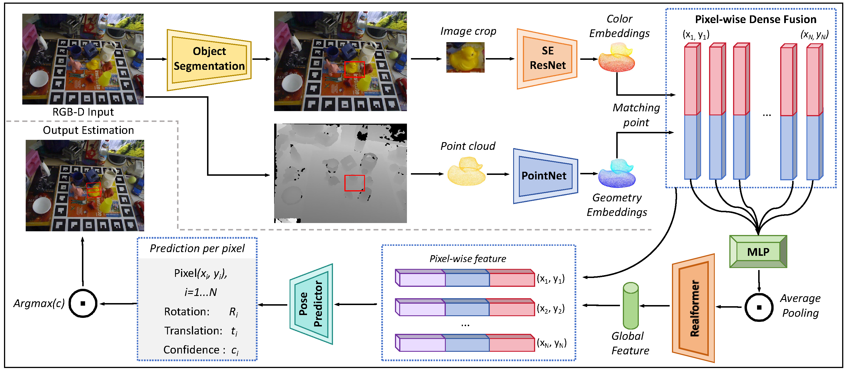
Figure 1.
The overall architecture of the proposed RAFusion network. The pipeline fuses RGB and depth features extracted by an SE-ResNet and a PointNet, respectively. A RealFormer module is inserted between pixel-wise fusion and average pooling; the pooled global context is concatenated with context-enhanced point features for pose and confidence prediction. Red squares mark the corresponding target region in the RGB and depth views, colored feature bars distinguish color and geometry embeddings, and arrows indicate the direction of data flow.
Figure 1.
The overall architecture of the proposed RAFusion network. The pipeline fuses RGB and depth features extracted by an SE-ResNet and a PointNet, respectively. A RealFormer module is inserted between pixel-wise fusion and average pooling; the pooled global context is concatenated with context-enhanced point features for pose and confidence prediction. Red squares mark the corresponding target region in the RGB and depth views, colored feature bars distinguish color and geometry embeddings, and arrows indicate the direction of data flow.
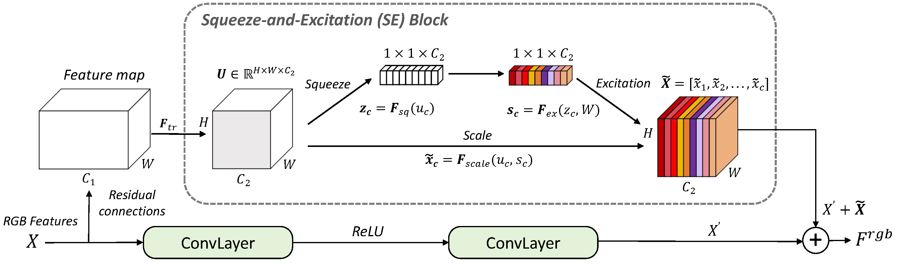
Figure 2.
SE-enhanced residual block for adaptive color feature extraction. In each ResNet-18 residual block, the SE operation is applied after the second convolution and before residual addition. The SE block computes channel-wise weights , and the recalibrated residual features are combined with the skip connection to produce . Colored bars depict channel responses and channel weights, arrows indicate feature flow, and the circled plus sign denotes residual addition.
Figure 2.
SE-enhanced residual block for adaptive color feature extraction. In each ResNet-18 residual block, the SE operation is applied after the second convolution and before residual addition. The SE block computes channel-wise weights , and the recalibrated residual features are combined with the skip connection to produce . Colored bars depict channel responses and channel weights, arrows indicate feature flow, and the circled plus sign denotes residual addition.
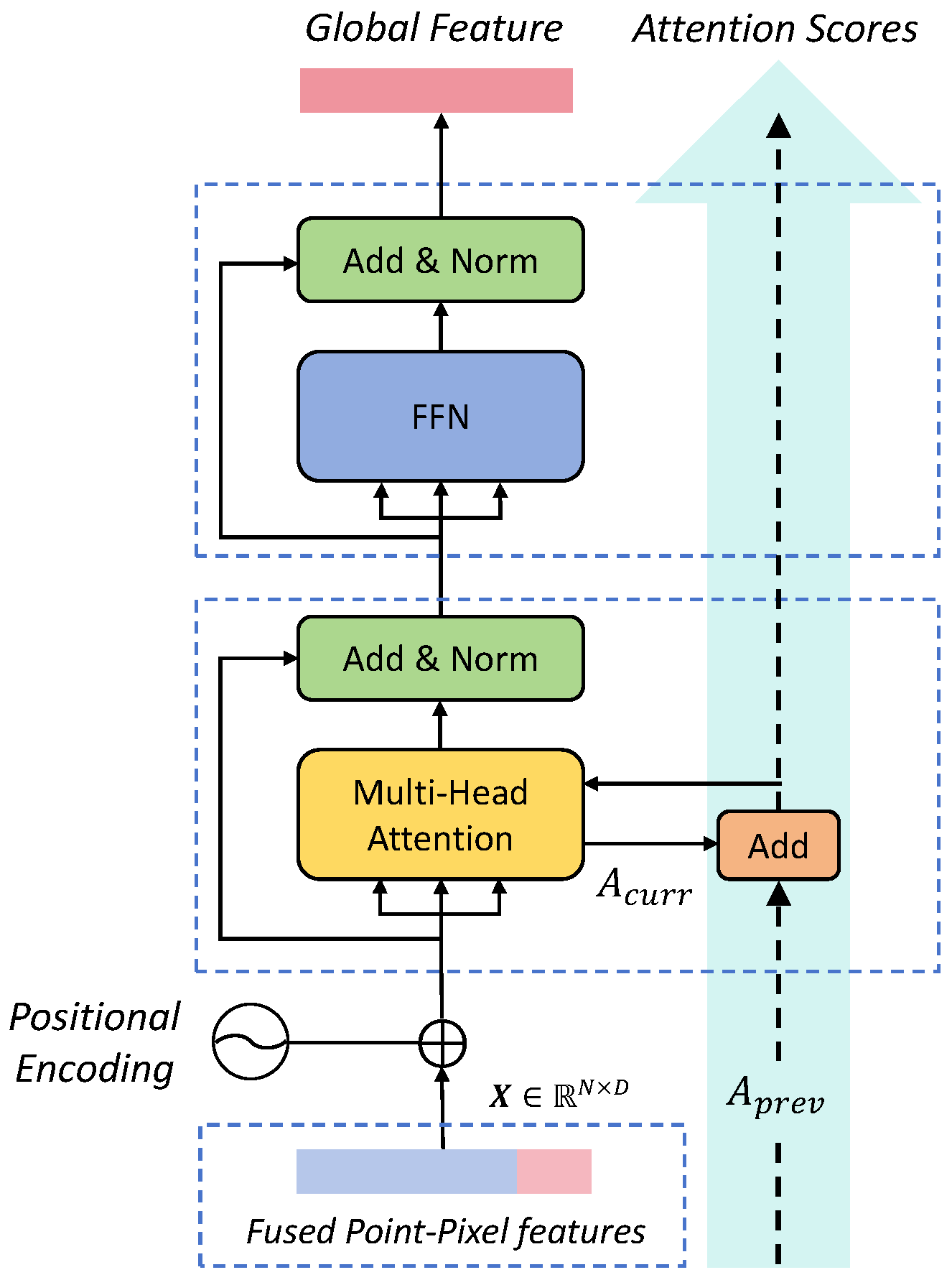
Figure 3.
Structure of the RealFormer-based global fusion module. Positionally encoded features pass through a Transformer layer in which the residual-attention path adds the previous pre-softmax logits to the current logits . The resulting attention weights support the accumulation of global context across layers. Colored boxes denote processing blocks, solid arrows show feature flow, and the vertical dashed arrow indicates the residual attention-score path.
Figure 3.
Structure of the RealFormer-based global fusion module. Positionally encoded features pass through a Transformer layer in which the residual-attention path adds the previous pre-softmax logits to the current logits . The resulting attention weights support the accumulation of global context across layers. Colored boxes denote processing blocks, solid arrows show feature flow, and the vertical dashed arrow indicates the residual attention-score path.
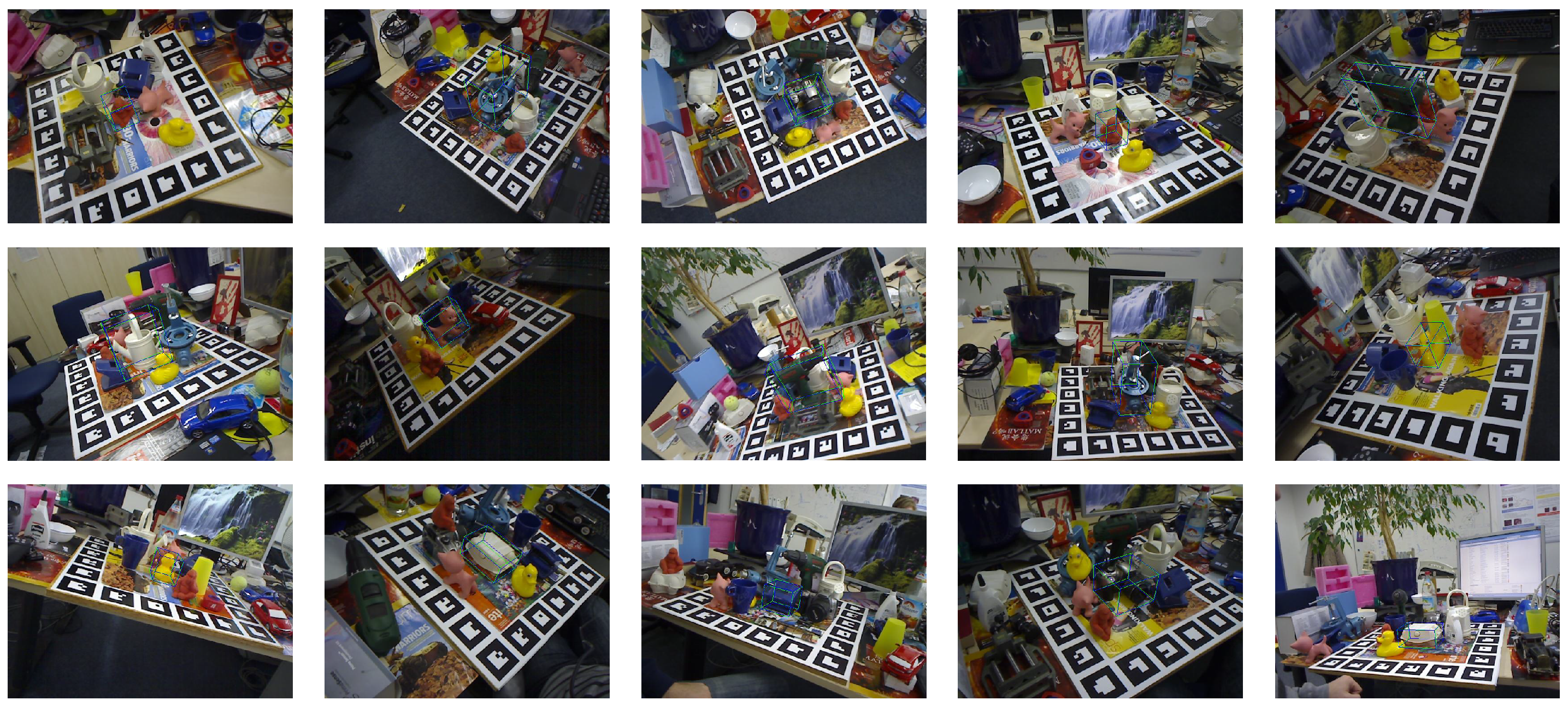
Figure 4.
Qualitative results of RAFusion on the LINEMOD dataset. The predictions show close visual alignment across varying viewpoints and cluttered backgrounds. The green bounding boxes represent the ground truth, while the blue bounding boxes represent the pose predictions output by RAFusion.
Figure 4.
Qualitative results of RAFusion on the LINEMOD dataset. The predictions show close visual alignment across varying viewpoints and cluttered backgrounds. The green bounding boxes represent the ground truth, while the blue bounding boxes represent the pose predictions output by RAFusion.
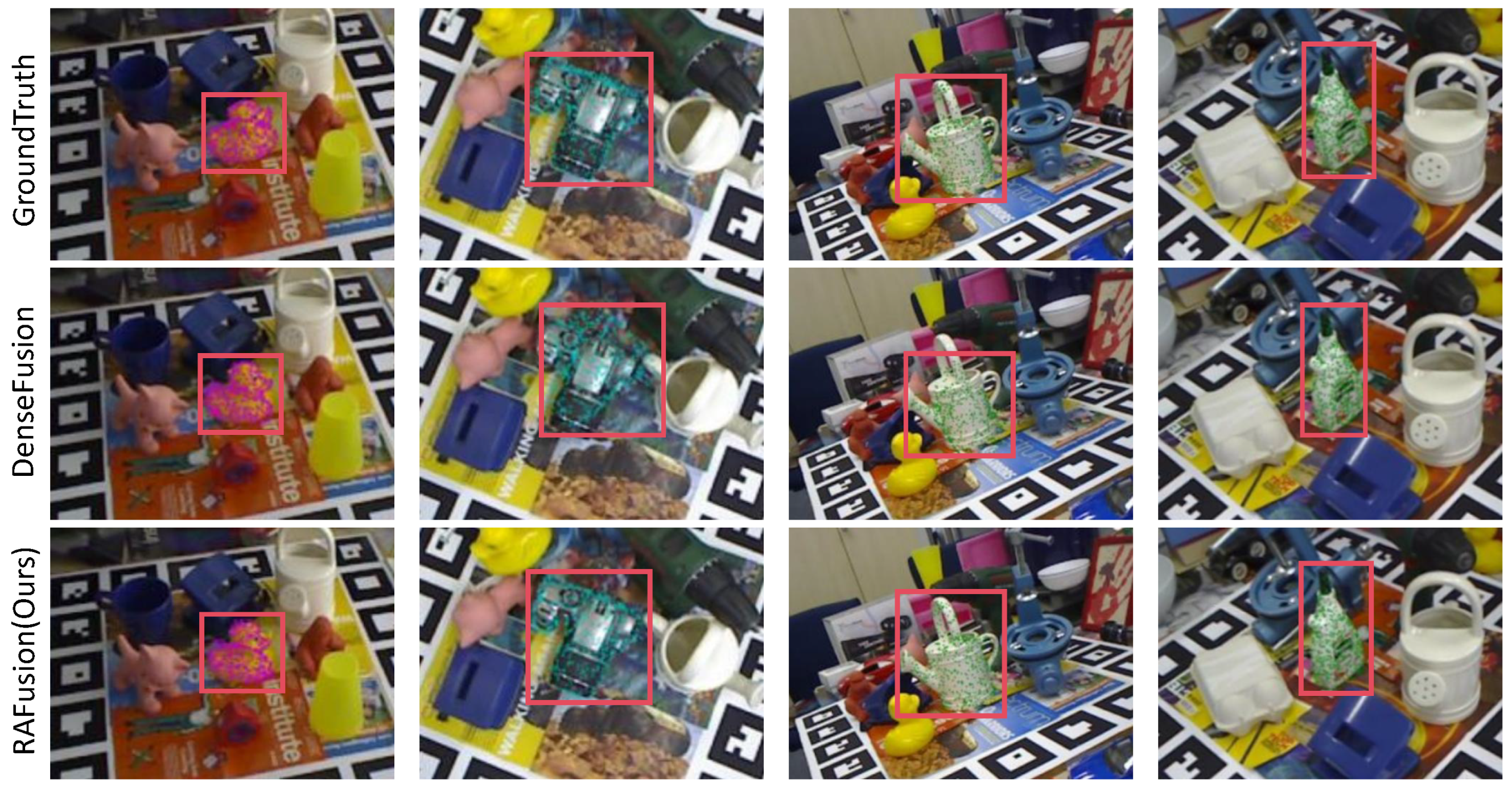
Figure 5.
Qualitative comparison of pose estimation results. Each column shows one test example. The first row is the ground-truth pose, the second row is the DenseFusion prediction, and the third row is the RAFusion prediction. Pose accuracy is visualized via projected bounding boxes.
Figure 5.
Qualitative comparison of pose estimation results. Each column shows one test example. The first row is the ground-truth pose, the second row is the DenseFusion prediction, and the third row is the RAFusion prediction. Pose accuracy is visualized via projected bounding boxes.
Figure 6.
Representative failure cases of RAFusion on Occlusion LINEMOD. The four examples are arranged from left to right. Green and blue boxes denote ground-truth and RAFusion poses, respectively. The cases include severe occlusion and symmetry-induced ambiguity.
Figure 6.
Representative failure cases of RAFusion on Occlusion LINEMOD. The four examples are arranged from left to right. Green and blue boxes denote ground-truth and RAFusion poses, respectively. The cases include severe occlusion and symmetry-induced ambiguity.
Table 1.
Quantitative comparison on the LINEMOD dataset using the ADD-(S) metric (%). RAFusion achieves the highest reported mean accuracy in this table and improves over the DenseFusion baseline.
Table 1.
Quantitative comparison on the LINEMOD dataset using the ADD-(S) metric (%). RAFusion achieves the highest reported mean accuracy in this table and improves over the DenseFusion baseline.
| | RGB-Based Input | RGB-D Input |
|---|
| Object | Trans6D+ [40] | GS-Pose [41] | PoseMatcher [42] | PointFusion [12,43] | PVN3D [11] | DenseFusion [12] | RAFusion (Ours) |
|---|
| ape | 88.3 | 71.0 | 59.2 | 70.4 | 95.5 | 92.3 | 94.1 |
| benchvise | 99.4 | 99.8 | 98.1 | 80.7 | 94.5 | 93.2 | 97.4 |
| cam | 97.8 | 98.2 | 93.4 | 60.8 | 94.2 | 94.4 | 98.7 |
| can | 99.1 | 97.7 | 96.0 | 61.1 | 94.3 | 93.1 | 97.4 |
| cat | 93.2 | 86.7 | 88.0 | 79.1 | 95.5 | 96.5 | 98.0 |
| driller | 99.5 | 96.2 | 98.4 | 47.3 | 93.3 | 87.0 | 95.0 |
| duck | 87.8 | 77.2 | 54.1 | 63.0 | 94.6 | 92.3 | 96.2 |
| eggbox | 100.0 | 99.6 | 97.8 | 99.9 | 100.0 | 99.8 | 100.0 |
| glue | 99.8 | 98.4 | 91.5 | 99.3 | 100.0 | 100.0 | 100.0 |
| holepuncher | 96.7 | 98.8 | 87.9 | 96.3 | 95.1 | 92.1 | 96.7 |
| iron | 99.9 | 99.6 | 94.0 | 97.2 | 96.3 | 97.0 | 99.2 |
| lamp | 99.7 | 98.9 | 98.1 | 62.3 | 93.7 | 95.3 | 98.7 |
| phone | 99.5 | 85.0 | 92.1 | 78.8 | 93.6 | 92.8 | 97.6 |
| Mean | 96.9 | 92.0 | 87.5 | 73.7 | 95.1 | 94.3 | 97.6 |
Table 2.
Quantitative comparison on the LINEMOD dataset using the 2D reprojection metric (%, 5-pixel threshold). RAFusion attains the highest reported mean accuracy among the listed RGB-D methods and improves over the DenseFusion baseline by 4.3 percentage points.
Table 2.
Quantitative comparison on the LINEMOD dataset using the 2D reprojection metric (%, 5-pixel threshold). RAFusion attains the highest reported mean accuracy among the listed RGB-D methods and improves over the DenseFusion baseline by 4.3 percentage points.
| | RGB | RGB-D |
|---|
| Obj. | BB8 [39] | GS-Pose [41] | DIM [7] | DF [12] | RAF |
|---|
| ape | 96.6 | 97.9 | 98.4 | 96.9 | 97.7 |
| benchvise | 90.1 | 98.9 | 97.0 | 88.3 | 94.8 |
| cam | 86.0 | 99.1 | 98.9 | 93.8 | 98.9 |
| can | 91.2 | 97.6 | 99.7 | 96.1 | 98.6 |
| cat | 98.8 | 98.9 | 98.7 | 96.1 | 99.4 |
| driller | 80.9 | 93.7 | 96.1 | 84.8 | 96.8 |
| duck | 92.2 | 97.8 | 98.5 | 98.5 | 98.9 |
| eggbox | 91.0 | 97.1 | 96.2 | 99.3 | 100.0 |
| glue | 92.3 | 97.4 | 98.9 | 95.5 | 99.9 |
| holepuncher | 95.3 | 98.8 | 96.3 | 87.9 | 95.9 |
| iron | 84.8 | 99.6 | 97.2 | 94.0 | 96.3 |
| lamp | 75.8 | 94.2 | 94.2 | 92.3 | 96.9 |
| phone | 85.3 | 93.8 | 97.7 | 93.0 | 98.7 |
| Mean | 89.3 | 97.3 | 97.5 | 93.6 | 97.9 |
Table 3.
Controlled overall comparison on the Occlusion LINEMOD dataset. DenseFusion and RAFusion checkpoints are evaluated on the same 1445 target instances using the same local evaluation protocol.
Table 3.
Controlled overall comparison on the Occlusion LINEMOD dataset. DenseFusion and RAFusion checkpoints are evaluated on the same 1445 target instances using the same local evaluation protocol.
| Model | ADD-(S) (%) | 2D Reprojection (%) | Targets |
|---|
| DenseFusion | 40.14 | 17.85 | 1445 |
| RAFusion (ours) | 57.92 | 28.37 | 1445 |
Table 4.
Sensitivity to stochastic point sampling on Occlusion LINEMOD. Using the same fixed checkpoint, values are reported as mean plus or minus standard deviation over inference sampling seeds 2026, 2027, and 2028.
Table 4.
Sensitivity to stochastic point sampling on Occlusion LINEMOD. Using the same fixed checkpoint, values are reported as mean plus or minus standard deviation over inference sampling seeds 2026, 2027, and 2028.
| Model | ADD-(S) (%) | 2D Reprojection (%) |
|---|
| DenseFusion | | |
| RAFusion (ours) | | |
Table 5.
Computational efficiency comparison. FLOPs and latency correspond to one PoseNet estimator forward pass under the same hardware and input settings.
Table 5.
Computational efficiency comparison. FLOPs and latency correspond to one PoseNet estimator forward pass under the same hardware and input settings.
| Model | Params (M) | FLOPs (G) | Latency (ms) | FPS |
|---|
| DenseFusion baseline | 21.370 | 13.488 | 1.780 | 561.803 |
| DenseFusion + SE | 21.457 | 13.490 | 1.883 | 531.171 |
| DenseFusion + RealFormer | 47.335 | 26.356 | 2.770 | 361.048 |
| RAFusion | 47.422 | 26.358 | 2.900 | 344.861 |
Table 6.
Ablation study of different components on the LINEMOD dataset. The results show that both the SE block and the RealFormer module contribute to the performance improvement, with the full RAFusion model achieving the highest accuracy. A checkmark indicates that the corresponding module is included, whereas – indicates that it is not included.
Table 6.
Ablation study of different components on the LINEMOD dataset. The results show that both the SE block and the RealFormer module contribute to the performance improvement, with the full RAFusion model achieving the highest accuracy. A checkmark indicates that the corresponding module is included, whereas – indicates that it is not included.
| Method | SE | RealFormer | ADD-(S) |
|---|
| Baseline (DenseFusion) | – | – | 94.3% |
| Baseline + SE | ✓ | – | 95.8% |
| Baseline + RealFormer | – | ✓ | 96.5% |
| RAFusion (ours) | ✓ | ✓ | 97.6% |
Table 7.
Hyperparameter sensitivity analysis. Impact of RealFormer depth (L) and SE reduction ratio (r) on accuracy.
Table 7.
Hyperparameter sensitivity analysis. Impact of RealFormer depth (L) and SE reduction ratio (r) on accuracy.
| RealFormer Depth L | SE Reduction Ratio r |
|---|
| Value | ADD-(S) | Value | ADD-(S) |
|---|
| 96.9% | | 97.5% |
| 97.6% | | 97.6% |
| 97.4% | | 97.1% |