Figure 1.
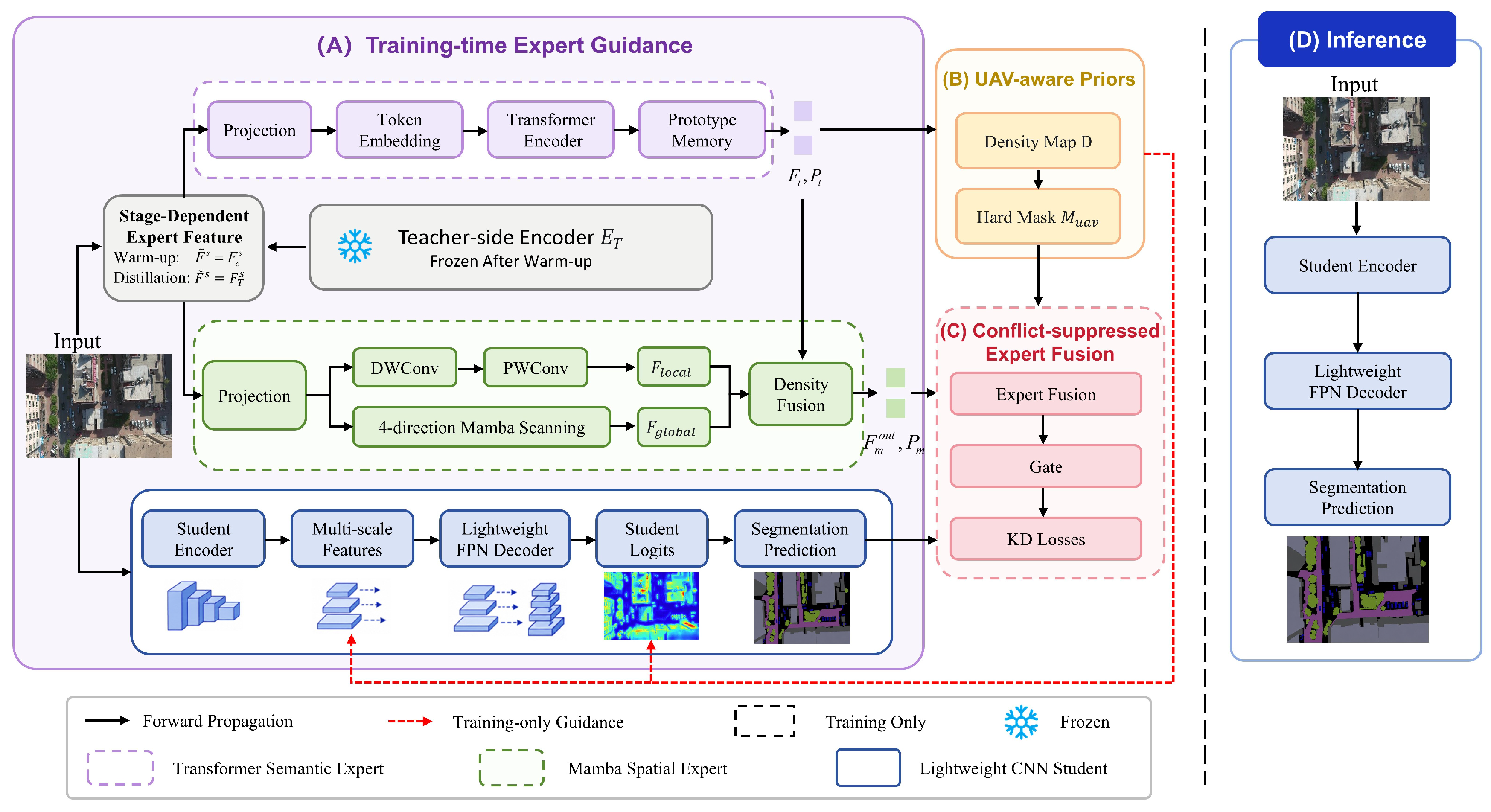
Overall architecture of MEKD-UAVSeg. During training, Transformer and Mamba experts provide complementary semantic and spatial guidance to a lightweight CNN student through UAV-aware priors and conflict-suppressed expert fusion. During inference, all expert branches, prior modules, routing modules, and distillation losses are discarded, leaving only the lightweight CNN student for semantic perception.
Figure 1.
Overall architecture of MEKD-UAVSeg. During training, Transformer and Mamba experts provide complementary semantic and spatial guidance to a lightweight CNN student through UAV-aware priors and conflict-suppressed expert fusion. During inference, all expert branches, prior modules, routing modules, and distillation losses are discarded, leaving only the lightweight CNN student for semantic perception.
Figure 2.
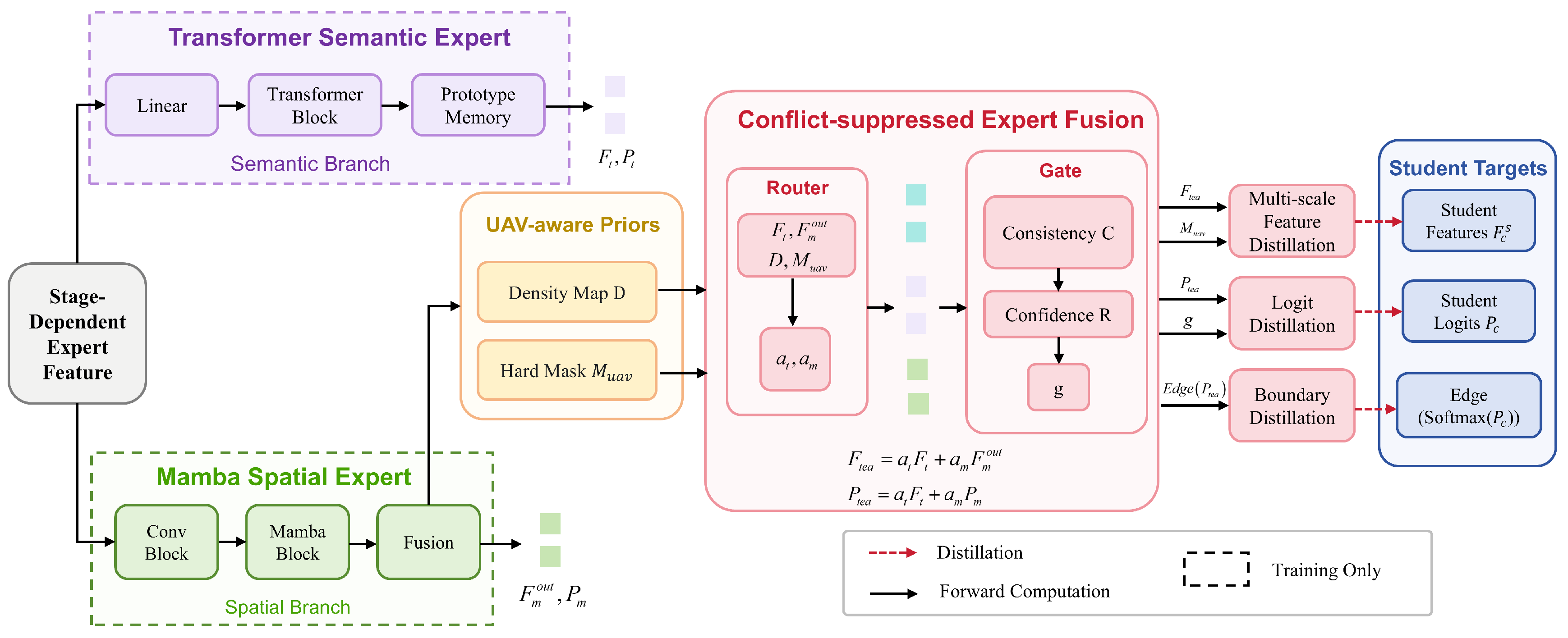
Architecture of the heterogeneous expert fusion and conflict-suppressed distillation module in MEKD-UAVSeg. The figure illustrates the Transformer semantic expert, Mamba spatial expert, UAV-aware priors, expert router, consistency–confidence gate, and student targets, where reliable expert cues are transferred to the student through logit, multi-scale feature, and boundary distillation.
Figure 2.
Architecture of the heterogeneous expert fusion and conflict-suppressed distillation module in MEKD-UAVSeg. The figure illustrates the Transformer semantic expert, Mamba spatial expert, UAV-aware priors, expert router, consistency–confidence gate, and student targets, where reliable expert cues are transferred to the student through logit, multi-scale feature, and boundary distillation.
Figure 3.
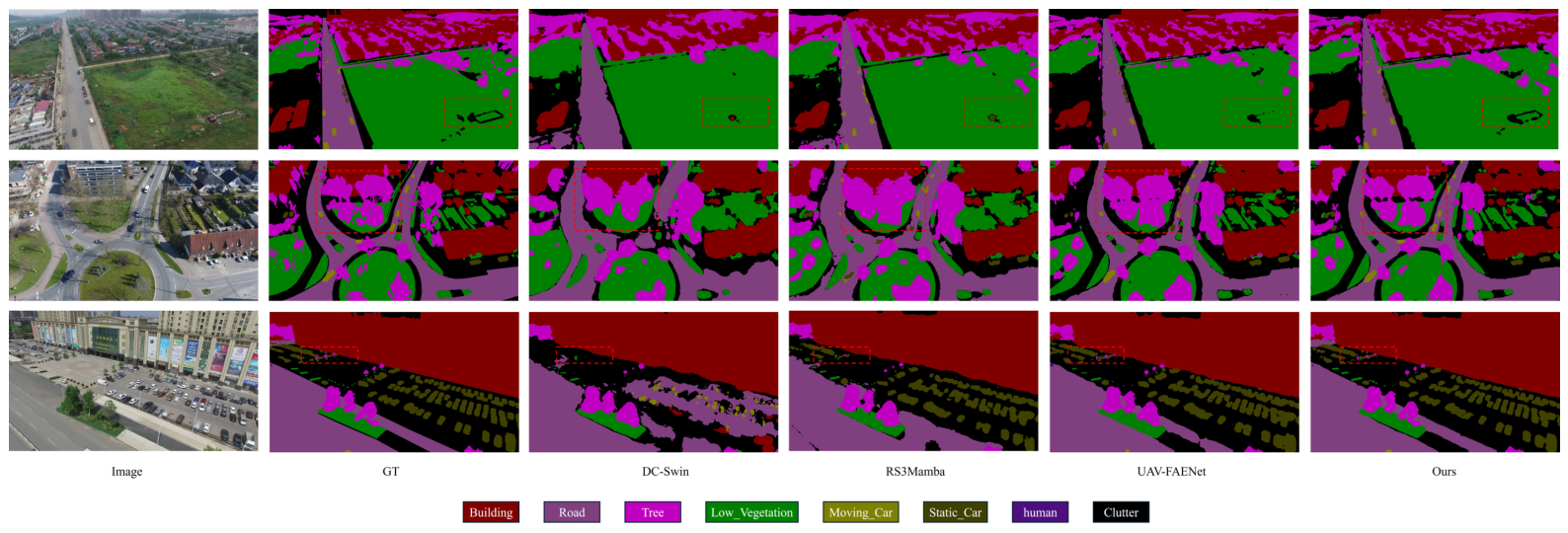
Qualitative comparison on the UAVid dataset. From left to right, each row shows the input image, ground truth, DC-Swin, RS3Mamba, UAV-FAENet, and the proposed MEKD-UAVSeg. The dashed boxes indicate challenging regions where MEKD-UAVSeg better preserves road boundaries, vegetation structures, small vehicles, and cluttered urban details.
Figure 3.
Qualitative comparison on the UAVid dataset. From left to right, each row shows the input image, ground truth, DC-Swin, RS3Mamba, UAV-FAENet, and the proposed MEKD-UAVSeg. The dashed boxes indicate challenging regions where MEKD-UAVSeg better preserves road boundaries, vegetation structures, small vehicles, and cluttered urban details.
Figure 4.
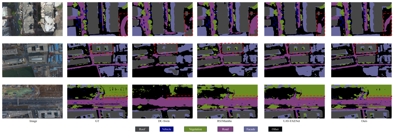
Qualitative comparison on the UDD6 dataset. From left to right, each row shows the input image, ground truth, DC-Swin, RS3Mamba, UAV-FAENet, and the proposed MEKD-UAVSeg. Compared with representative Transformer-, Mamba-, and hybrid-based methods, MEKD-UAVSeg better preserves structural boundaries and local object regions, such as roads, roofs, vehicles, vegetation, and facades. Red dashed boxes indicate challenging regions with small objects, ambiguous appearances, or complex spatial layouts.
Figure 4.
Qualitative comparison on the UDD6 dataset. From left to right, each row shows the input image, ground truth, DC-Swin, RS3Mamba, UAV-FAENet, and the proposed MEKD-UAVSeg. Compared with representative Transformer-, Mamba-, and hybrid-based methods, MEKD-UAVSeg better preserves structural boundaries and local object regions, such as roads, roofs, vehicles, vegetation, and facades. Red dashed boxes indicate challenging regions with small objects, ambiguous appearances, or complex spatial layouts.
Figure 5.
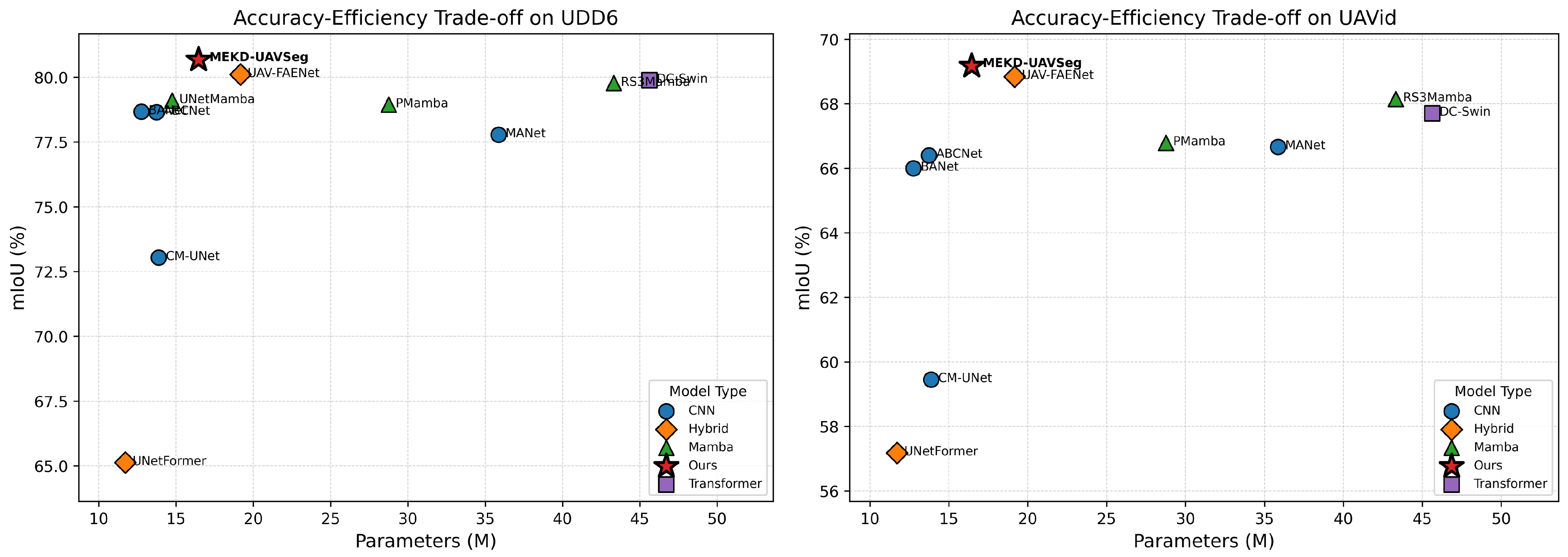
Accuracy–efficiency trade-off on UDD6 and UAVid. The horizontal axis denotes the number of inference-stage parameters, and the vertical axis denotes mean Intersection over Union (mIoU). Each point represents a segmentation method. MEKD-UAVSeg achieves higher segmentation accuracy with a compact inference model because the Transformer and Mamba experts are used only during training and removed after distillation.
Figure 5.
Accuracy–efficiency trade-off on UDD6 and UAVid. The horizontal axis denotes the number of inference-stage parameters, and the vertical axis denotes mean Intersection over Union (mIoU). Each point represents a segmentation method. MEKD-UAVSeg achieves higher segmentation accuracy with a compact inference model because the Transformer and Mamba experts are used only during training and removed after distillation.
Table 1.
Quantitative comparison of different methods on the UAVid dataset. For the proposed method, we report the mean and standard deviation over multiple runs. For competing methods, we report reproduced or officially reported results under the same evaluation protocol. The best and second-best segmentation results are highlighted in bold and underlined, respectively.
Table 1.
Quantitative comparison of different methods on the UAVid dataset. For the proposed method, we report the mean and standard deviation over multiple runs. For competing methods, we report reproduced or officially reported results under the same evaluation protocol. The best and second-best segmentation results are highlighted in bold and underlined, respectively.
| Method | Type | IoU (%) | mIoU (%) | mF1 (%) | OA (%) | Param (M) |
|---|
|
Building
|
Road
|
Tree
|
LowVeg
|
MovingCar
|
StaticCar
|
Human
|
Clutter
|
|---|
| ABCNet [7] | CNN | 85.77 | 80.92 | 77.88 | 62.46 | 74.12 | 53.33 | 29.29 | 66.14 | 66.40 | 78.13 | 85.48 | 13.74 |
| BANet [45] | CNN | 83.90 | 81.48 | 78.51 | 62.18 | 77.44 | 52.01 | 29.51 | 64.58 | 66.00 | 77.86 | 84.99 | 12.76 |
| MANet [46] | CNN | 84.42 | 80.17 | 78.75 | 62.39 | 68.73 | 62.73 | 29.40 | 66.17 | 66.66 | 78.50 | 85.19 | 35.86 |
| DC-Swin [47] | Transformer | 87.64 | 82.49 | 79.78 | 64.64 | 76.02 | 53.62 | 29.72 | 68.43 | 67.70 | 79.01 | 86.58 | 45.63 |
| UNetFormer [8] | Hybrid | 75.38 | 75.36 | 72.11 | 56.95 | 64.57 | 35.89 | 20.03 | 55.86 | 57.18 | 70.42 | 79.75 | 11.72 |
| CM-UNet [48] | CNN | 79.05 | 78.71 | 73.55 | 56.85 | 69.71 | 33.64 | 24.64 | 59.30 | 59.45 | 72.24 | 81.59 | 13.88 |
| RS3Mamba [39] | Mamba | 86.54 | 81.83 | 79.03 | 63.10 | 75.79 | 60.42 | 30.36 | 67.22 | 68.15 | 79.51 | 86.01 | 43.32 |
| PMamba [49] | Mamba | 85.93 | 81.20 | 78.66 | 62.38 | 73.95 | 56.45 | 28.96 | 66.48 | 66.79 | 78.43 | 85.59 | 28.76 |
| UAV-FAENet [31] | Hybrid | 87.37 | 83.20 | 79.26 | 63.54 | 78.02 | 59.53 | 30.98 | 68.25 | 68.84 | 79.97 | 86.48 | 19.17 |
| MEKD-UAVSeg (Ours) | Hybrid | 87.92 | 83.05 | 79.41 | 65.10 | 77.85 | 61.28 | 30.65 | 68.10 | | | | 16.45 |
Table 2.
Quantitative comparison results on the UDD6 dataset. For the proposed method, we report the mean and standard deviation over multiple runs. For competing methods, we report reproduced or officially reported results under the same evaluation protocol. The best and second-best segmentation results are highlighted in bold and underlined, respectively.
Table 2.
Quantitative comparison results on the UDD6 dataset. For the proposed method, we report the mean and standard deviation over multiple runs. For competing methods, we report reproduced or officially reported results under the same evaluation protocol. The best and second-best segmentation results are highlighted in bold and underlined, respectively.
| Methods | Type | IoU (%) | mIoU (%) | mF1 (%) | OA (%) | Param (M) |
|---|
| Facade | Road | Vegetation | Vehicle | Roof | Other |
|---|
| ABCNet [7] | CNN | 73.10 | 70.05 | 89.79 | 71.64 | 88.68 | 63.27 | 78.65 | 87.76 | 88.13 | 13.74 |
| BANet [45] | CNN | 73.72 | 70.59 | 89.52 | 71.75 | 87.77 | 62.96 | 78.67 | 87.83 | 88.03 | 12.76 |
| MANet [46] | CNN | 72.53 | 68.84 | 89.49 | 70.37 | 87.64 | 62.58 | 77.78 | 87.22 | 87.58 | 35.86 |
| DC-Swin [47] | Transformer | 75.50 | 73.03 | 89.72 | 72.08 | 89.14 | 64.95 | 79.89 | 88.61 | 88.95 | 45.63 |
| UNetFormer [8] | Hybrid | 55.87 | 58.40 | 87.16 | 48.16 | 76.08 | 50.20 | 65.13 | 78.00 | 80.39 | 11.72 |
| CM-UNet [48] | CNN | 64.76 | 66.26 | 88.88 | 60.38 | 84.94 | 55.71 | 73.04 | 83.91 | 85.06 | 13.88 |
| RS3Mamba [39] | Mamba | 75.46 | 72.14 | 89.68 | 72.01 | 89.57 | 64.44 | 79.77 | 88.52 | 88.87 | 43.32 |
| PMamba [49] | Mamba | 74.30 | 71.04 | 89.31 | 70.97 | 89.06 | 63.79 | 78.94 | 87.98 | 88.38 | 28.76 |
| UNetMamba [41] | Mamba | 73.52 | 71.17 | 89.33 | 72.71 | 88.78 | 63.22 | 79.10 | 88.10 | 88.19 | 14.75 |
| UAV-FAENet [31] | Hybrid | 75.39 | 72.43 | 89.58 | 73.27 | 89.89 | 63.78 | 80.11 | 88.74 | 88.80 | 19.17 |
| MEKD-UAVSeg (Ours) | Hybrid | 76.52 | 73.85 | 89.60 | 73.60 | 89.85 | 64.90 | | | | 16.45 |
Table 3.
Comparison with existing distillation strategies on UAVid and UDD6. All methods use the same STDC2-FPN student for inference. The best and second-best results are highlighted in bold and underlined, respectively.
Table 3.
Comparison with existing distillation strategies on UAVid and UDD6. All methods use the same STDC2-FPN student for inference. The best and second-best results are highlighted in bold and underlined, respectively.
| Method | UAVid | UDD6 |
|---|
| mIoU | mF1 | OA | mIoU | mF1 | OA |
|---|
| Student only | 66.45 | 77.82 | 84.90 | 77.50 | 87.10 | 87.20 |
| Vanilla KD [50] | 67.15 | 78.40 | 85.35 | 78.30 | 87.65 | 87.75 |
| CWD [15] | 67.68 | 78.95 | 85.70 | 78.90 | 88.05 | 88.25 |
| CIRKD [16] | 67.42 | 78.70 | 85.55 | 78.65 | 87.85 | 88.00 |
| BPKD [22] | 68.35 | 79.50 | 86.05 | 79.85 | 88.50 | 88.65 |
| BRD [23] | 68.05 | 79.25 | 85.90 | 79.50 | 88.30 | 88.45 |
| MEKD-UAVSeg (Ours) | 69.17 | 80.35 | 86.62 | 80.68 | 88.95 | 89.12 |
Table 4.
Efficiency comparison on the UAVid dataset. FPS, GFLOPs, latency, parameters, mIoU, and mF1 are reported to evaluate the accuracy–efficiency trade-off of different methods. All efficiency results are measured under the same GPU, input resolution, batch size, precision setting, warm-up protocol, and repeated forward-pass protocol. For the proposed framework, all training-only expert branches and distillation modules are removed during measurement, and only the deployed CNN student is retained.
Table 4.
Efficiency comparison on the UAVid dataset. FPS, GFLOPs, latency, parameters, mIoU, and mF1 are reported to evaluate the accuracy–efficiency trade-off of different methods. All efficiency results are measured under the same GPU, input resolution, batch size, precision setting, warm-up protocol, and repeated forward-pass protocol. For the proposed framework, all training-only expert branches and distillation modules are removed during measurement, and only the deployed CNN student is retained.
| Method | FPS ↑ | GFLOPs ↓ | Latency (ms) ↓ | Param (M) ↓ | mIoU ↑ | mF1 ↑ |
|---|
| ABCNet [7] | 102.2 | 62.9 | 9.8 | 13.74 | 66.40 | 78.13 |
| BANet [45] | 37.3 | 107.2 | 26.8 | 12.76 | 66.00 | 77.86 |
| MANet [46] | 75.6 | 51.7 | 13.2 | 35.86 | 66.66 | 78.50 |
| DC-Swin [47] | 23.5 | 170.3 | 42.6 | 45.63 | 67.70 | 79.01 |
| UNetFormer [8] | 115.6 | 46.9 | 8.7 | 11.72 | 57.18 | 70.42 |
| CM-UNet [48] | 47.7 | 83.8 | 21.0 | 13.88 | 59.45 | 72.24 |
| RS3Mamba [39] | 17.7 | 226.0 | 56.5 | 43.32 | 68.15 | 79.51 |
| PMamba [49] | 49.9 | 80.2 | 20.0 | 28.76 | 66.79 | 78.43 |
| UAV-FAENet [31] | 52.0 | 76.9 | 19.2 | 19.17 | 68.84 | 79.97 |
| MEKD-UAVSeg (Ours) | 68.5 | 58.4 | 14.6 | 16.45 | 69.17 | 80.35 |
Table 5.
Hard-region evaluation on UAVid and UDD6. Small-object mIoU, rare-class mIoU, and boundary F-score are reported to evaluate the effectiveness of the proposed framework in difficult UAV regions. For UAVid, small-object mIoU is computed over MovingCar, StaticCar, and Human, while rare-class mIoU is computed over StaticCar, Human, and Clutter. Bold and underlined values indicate the best and second-best results, respectively.
Table 5.
Hard-region evaluation on UAVid and UDD6. Small-object mIoU, rare-class mIoU, and boundary F-score are reported to evaluate the effectiveness of the proposed framework in difficult UAV regions. For UAVid, small-object mIoU is computed over MovingCar, StaticCar, and Human, while rare-class mIoU is computed over StaticCar, Human, and Clutter. Bold and underlined values indicate the best and second-best results, respectively.
| Method | UAVid | UDD6 |
|---|
|
Small-Object mIoU
|
Rare-Class mIoU
|
Boundary F-Score
|
Vehicle IoU
|
Boundary F-Score
|
Foreground mIoU
|
|---|
| Student only | 51.20 | 48.35 | 63.40 | 68.20 | 70.55 | 77.50 |
| UAV-FAENet [31] | 56.18 | 52.92 | 68.85 | 73.27 | 74.60 | 80.11 |
| RS3Mamba [39] | 55.52 | 52.67 | 68.20 | 72.01 | 73.85 | 79.77 |
| MEKD-UAVSeg | 56.59 | 53.34 | 70.15 | 73.60 | 75.42 | 80.68 |
Table 6.
Component ablation of MEKD-UAVSeg on UAVid and UDD6. All variants use the same STDC2-FPN student during inference. Bold values indicate the best results.
Table 6.
Component ablation of MEKD-UAVSeg on UAVid and UDD6. All variants use the same STDC2-FPN student during inference. Bold values indicate the best results.
| Configuration | UAVid | UDD6 |
|---|
|
mIoU
|
mF1
|
OA
|
mIoU
|
mF1
|
OA
|
|---|
| STDC2-FPN student | 66.45 | 77.82 | 84.90 | 77.50 | 87.10 | 87.20 |
| + Heterogeneous Transformer–Mamba experts | 67.12 | 78.45 | 85.35 | 78.35 | 87.65 | 87.75 |
| + Multi-scale cross-branch distillation | 67.68 | 78.90 | 85.62 | 79.05 | 88.10 | 88.20 |
| + UAV-aware density and hard-region priors | 68.15 | 79.35 | 85.90 | 79.52 | 88.42 | 88.55 |
| + Conflict-suppressed reliability routing | 68.54 | 79.72 | 86.15 | 80.05 | 88.68 | 88.80 |
| + Consistency and confidence gates | 68.92 | 80.08 | 86.40 | 80.40 | 88.82 | 88.98 |
| MEKD-UAVSeg (Full) | 69.17 | 80.35 | 86.62 | 80.68 | 88.95 | 89.12 |
Table 7.
Ablation on expert configurations. All variants use the same CNN student and training setting. For dual-expert variants, the fusion and distillation design is kept identical, and only the expert architecture is changed. Bold values indicate the best results.
Table 7.
Ablation on expert configurations. All variants use the same CNN student and training setting. For dual-expert variants, the fusion and distillation design is kept identical, and only the expert architecture is changed. Bold values indicate the best results.
| Expert Configuration | UAVid | UDD6 |
|---|
|
mIoU
|
mF1
|
OA
|
mIoU
|
mF1
|
OA
|
|---|
| Student only | 66.45 | 77.82 | 84.90 | 77.50 | 87.10 | 87.20 |
| Single Transformer expert | 66.98 | 78.30 | 85.25 | 78.10 | 87.50 | 87.60 |
| Single Mamba expert | 66.85 | 78.15 | 85.10 | 78.25 | 87.62 | 87.70 |
| Dual Transformer experts | 67.45 | 78.75 | 85.55 | 78.60 | 87.95 | 87.95 |
| Dual Mamba experts | 67.30 | 78.60 | 85.40 | 78.75 | 88.05 | 88.10 |
| Transformer + Mamba experts | 67.82 | 79.05 | 85.80 | 79.15 | 88.35 | 88.40 |
Table 8.
Comparison of different spatial expert designs. All variants use the same Transformer semantic expert, the same CNN student, and the same distillation setting. Only the spatial expert branch is changed, and all expert branches are removed during inference. Bold values indicate the best results.
Table 8.
Comparison of different spatial expert designs. All variants use the same Transformer semantic expert, the same CNN student, and the same distillation setting. Only the spatial expert branch is changed, and all expert branches are removed during inference. Bold values indicate the best results.
| Spatial Expert Design | UAVid | UDD6 |
|---|
|
mIoU
|
mF1
|
mIoU
|
mF1
|
|---|
| Dilated CNN expert | 68.86 | 80.05 | 80.36 | 88.73 |
| Lightweight attention expert | 68.97 | 80.14 | 80.45 | 88.80 |
| Mamba spatial expert | 69.17 | 80.35 | 80.68 | 88.95 |
Table 9.
Ablation study of different training protocols. All variants use the same model components and the same STDC2-FPN student for inference. Bold values indicate the best results.
Table 9.
Ablation study of different training protocols. All variants use the same model components and the same STDC2-FPN student for inference. Bold values indicate the best results.
| Training Protocol | Warm-Up | Expert KD | Frozen Source | UAVid | UDD6 |
|---|
| mIoU | mF1 | OA | mIoU | mF1 | OA |
|---|
| Student only | × | × | × | 66.45 | 77.82 | 84.90 | 77.50 | 87.10 | 87.20 |
| Direct KD | × | ✓ | × | 67.52 | 78.85 | 85.70 | 79.20 | 88.40 | 88.45 |
| Warm-up only | ✓ | × | × | 66.85 | 78.15 | 85.15 | 78.10 | 87.55 | 87.65 |
| Warm-up + online KD | ✓ | ✓ | × | 68.45 | 79.60 | 86.15 | 80.05 | 88.75 | 88.85 |
| Proposed two-stage KD | ✓ | ✓ | ✓ | 69.17 | 80.35 | 86.62 | 80.68 | 88.95 | 89.12 |
Table 10.
Feature-stability analysis of different training protocols. Cosine similarity is computed between teacher-side and student features at the last high-level feature stage during the distillation stage. Higher mean similarity and lower fluctuation indicate more stable teacher–student feature alignment. Bold values indicate the best results.
Table 10.
Feature-stability analysis of different training protocols. Cosine similarity is computed between teacher-side and student features at the last high-level feature stage during the distillation stage. Higher mean similarity and lower fluctuation indicate more stable teacher–student feature alignment. Bold values indicate the best results.
| Training Protocol | Feature Similarity ↑ | Similarity Std. ↓ | UAVid mIoU ↑ |
|---|
| Warm-up + online KD | 0.742 | 0.031 | 68.45 |
| Proposed two-stage KD | 0.816 | 0.018 | 69.17 |
Table 11.
Sensitivity analysis of the uncertainty-mask activation epoch . The uncertainty mask is disabled before and activated afterwards. Bold values indicate the best results.
Table 11.
Sensitivity analysis of the uncertainty-mask activation epoch . The uncertainty mask is disabled before and activated afterwards. Bold values indicate the best results.
| UAVid | UDD6 |
|---|
| mIoU | mF1 | mIoU | mF1 |
|---|
| 0 | 68.79 | 79.98 | 80.21 | 88.70 |
| 5 | 69.03 | 80.23 | 80.52 | 88.86 |
| 10 | 69.17 | 80.35 | 80.68 | 88.95 |
| 15 | 69.05 | 80.22 | 80.55 | 88.84 |
| 20 | 68.91 | 80.08 | 80.38 | 88.76 |
Table 12.
Sensitivity analysis of the consistency and confidence gate temperatures. Bold values indicate the best results.
Table 12.
Sensitivity analysis of the consistency and confidence gate temperatures. Bold values indicate the best results.
| | UAVid | UDD6 |
|---|
| mIoU | mF1 | mIoU | mF1 |
|---|
| 0.1 | 0.1 | 68.92 | 80.10 | 80.41 | 88.76 |
| 0.2 | 0.2 | 69.17 | 80.35 | 80.68 | 88.95 |
| 0.3 | 0.3 | 69.00 | 80.17 | 80.46 | 88.82 |
| 0.2 | 0.1 | 69.05 | 80.22 | 80.53 | 88.85 |
| 0.1 | 0.2 | 69.08 | 80.25 | 80.57 | 88.87 |
Table 13.
Sensitivity analysis of the Dice loss weight . Bold values indicate the best results.
Table 13.
Sensitivity analysis of the Dice loss weight . Bold values indicate the best results.
| UAVid | UDD6 |
|---|
| mIoU | mF1 | mIoU | mF1 |
|---|
| 0.25 | 69.02 | 80.18 | 80.49 | 88.82 |
| 0.50 | 69.17 | 80.35 | 80.68 | 88.95 |
| 1.00 | 68.96 | 80.12 | 80.43 | 88.78 |