Figure 1.
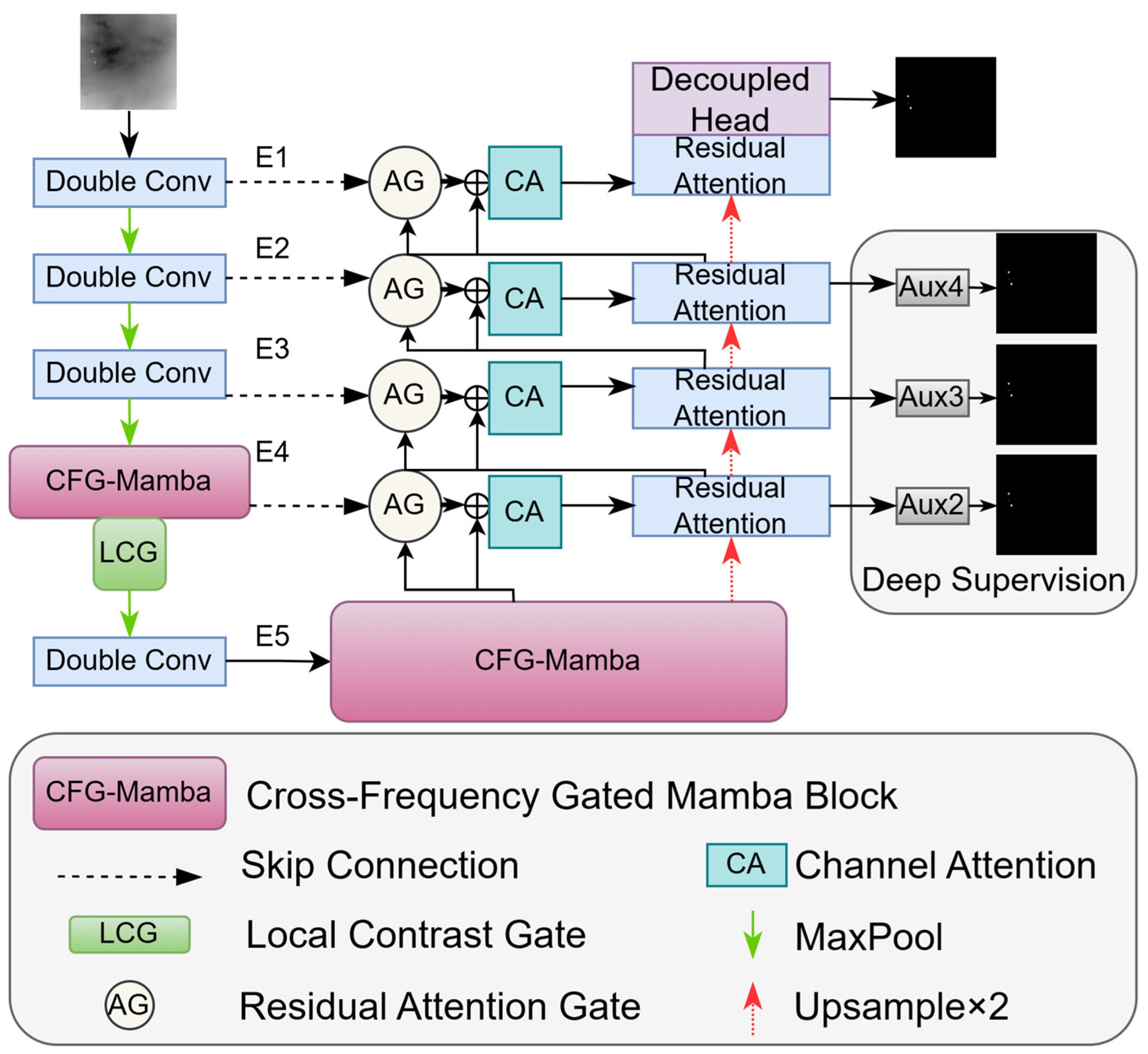
Overall architecture of the proposed CFGMNet. The network consists of a multi-scale encoder, two CFG-Mamba modules, a Local Contrast Gate, a residual attention decoder, and a decoupled prediction head. All components are trained from scratch without pre-trained weights or frozen layers.
Figure 1.
Overall architecture of the proposed CFGMNet. The network consists of a multi-scale encoder, two CFG-Mamba modules, a Local Contrast Gate, a residual attention decoder, and a decoupled prediction head. All components are trained from scratch without pre-trained weights or frozen layers.
Figure 2.
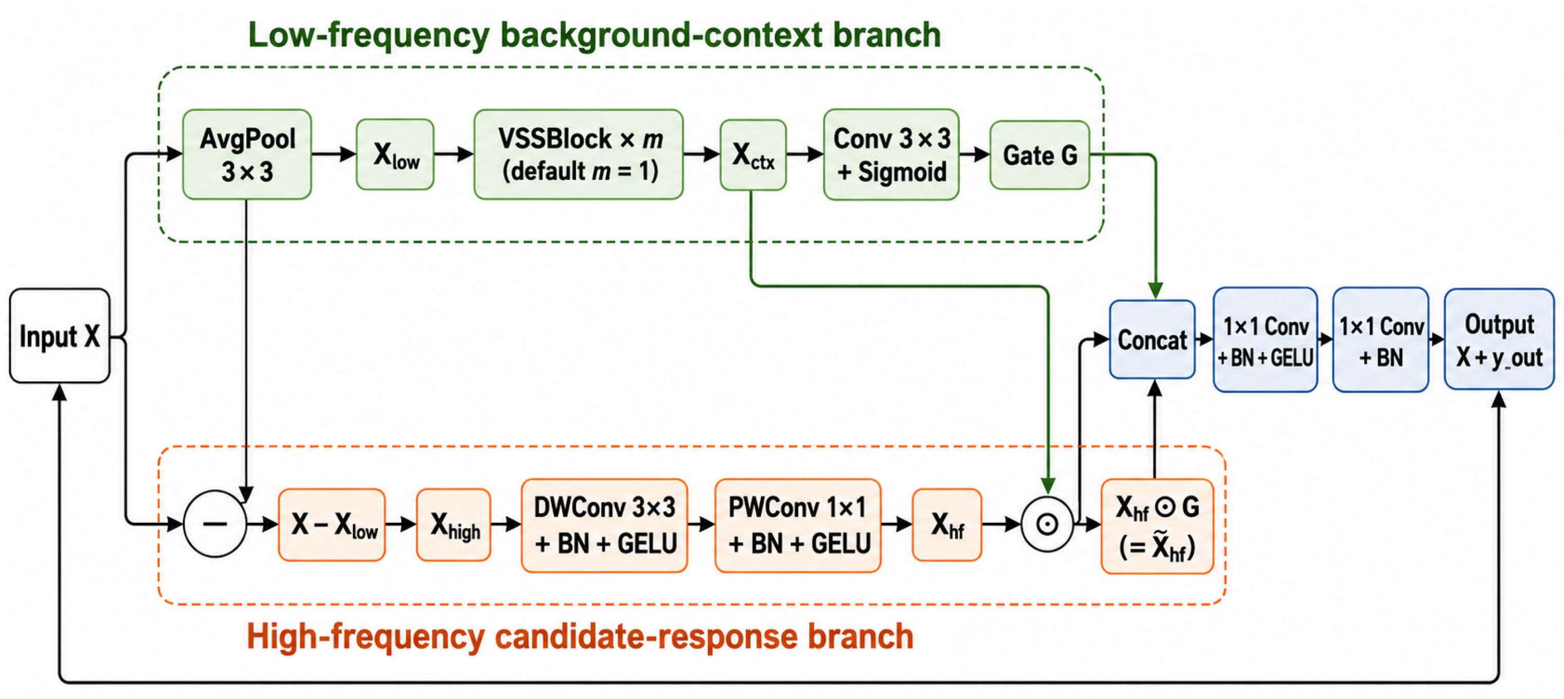
Structure of the Cross-Frequency Gated Mamba module. The input feature is decomposed into low-frequency background context and high-frequency candidate responses. The low-frequency branch generates a spatial gate to selectively verify high-frequency target-like responses.
Figure 2.
Structure of the Cross-Frequency Gated Mamba module. The input feature is decomposed into low-frequency background context and high-frequency candidate responses. The low-frequency branch generates a spatial gate to selectively verify high-frequency target-like responses.
Figure 3.
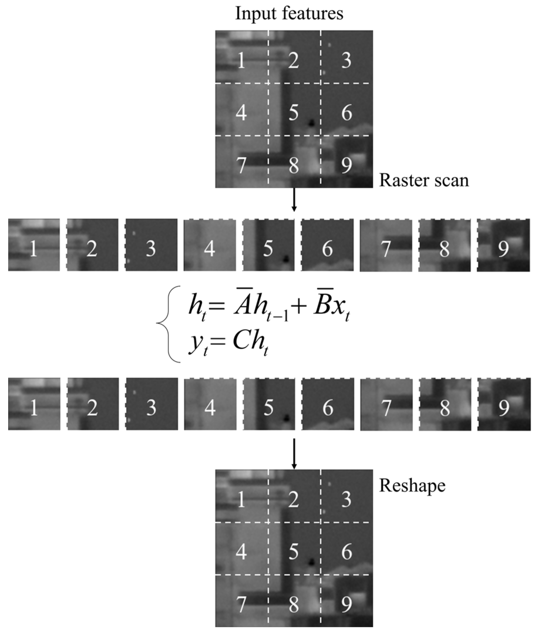
Sequence modeling process of the VSSBlock. The low-frequency feature map is serialized in row-major order, processed by LayerNorm and Mamba, and then reshaped back into a two-dimensional contextual feature map.
Figure 3.
Sequence modeling process of the VSSBlock. The low-frequency feature map is serialized in row-major order, processed by LayerNorm and Mamba, and then reshaped back into a two-dimensional contextual feature map.
Figure 4.
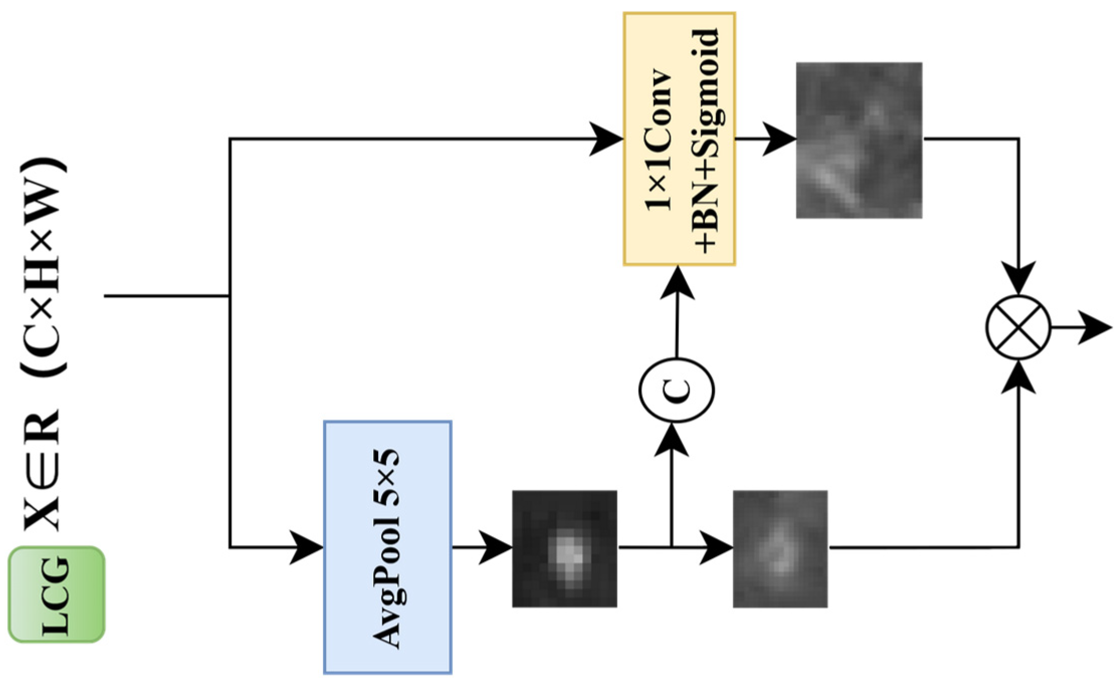
Structure of the Local Contrast Gate module. The module estimates local background responses and generates a contrast-aware spatial gate to suppress isolated background noise while preserving salient target candidates.
Figure 4.
Structure of the Local Contrast Gate module. The module estimates local background responses and generates a contrast-aware spatial gate to suppress isolated background noise while preserving salient target candidates.
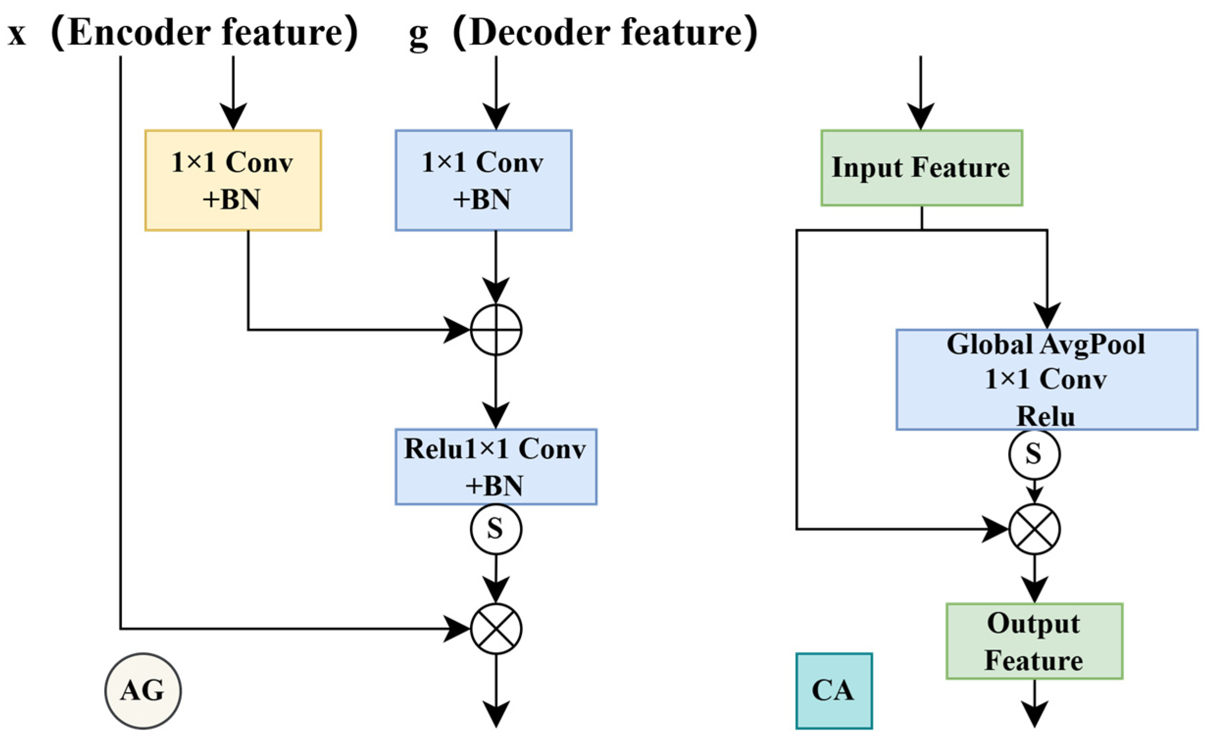
Figure 5.
Structure of the residual attention decoder. Decoder features guide the filtering of encoder skip-connection features, and residual channel attention further recalibrates the fused features to reduce background clutter.
Figure 5.
Structure of the residual attention decoder. Decoder features guide the filtering of encoder skip-connection features, and residual channel attention further recalibrates the fused features to reduce background clutter.
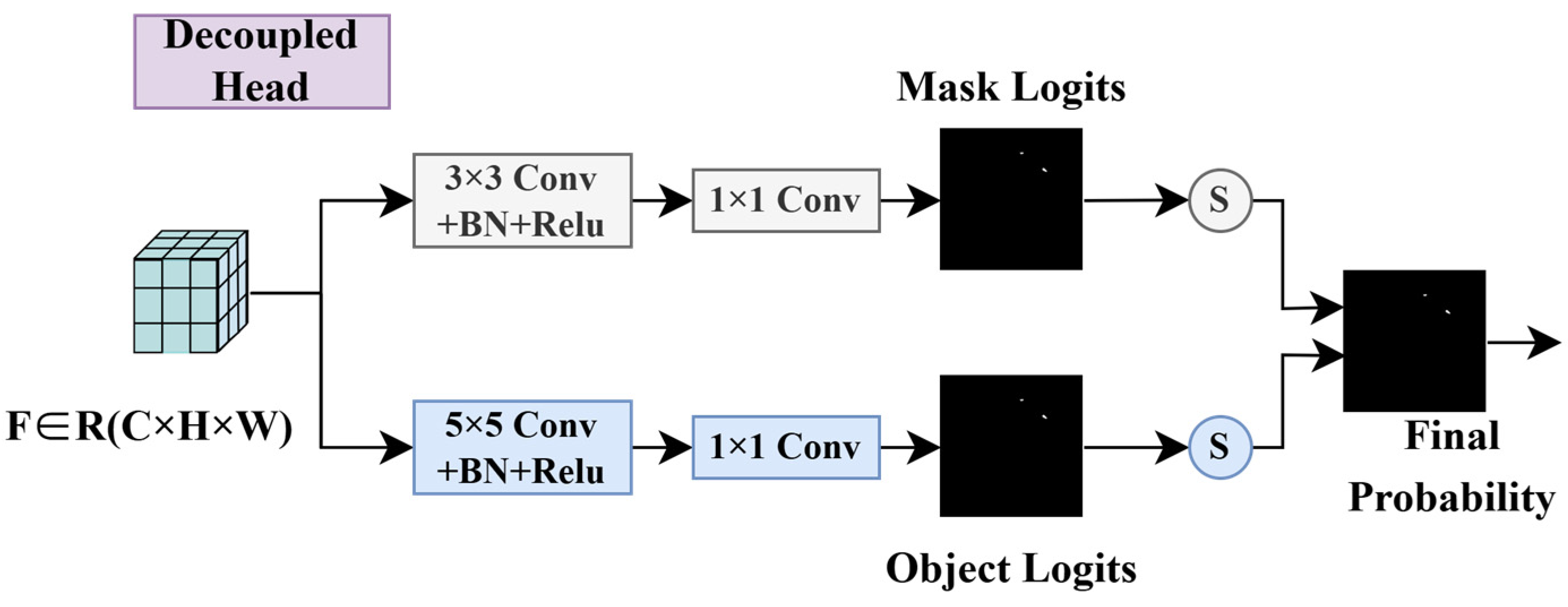
Figure 6.
Structure of the decoupled prediction head. The Mask branch predicts pixel-level target regions, while the Object branch verifies target presence. Their Sigmoid outputs are multiplied during inference to suppress isolated false responses.
Figure 6.
Structure of the decoupled prediction head. The Mask branch predicts pixel-level target regions, while the Object branch verifies target presence. Their Sigmoid outputs are multiplied during inference to suppress isolated false responses.
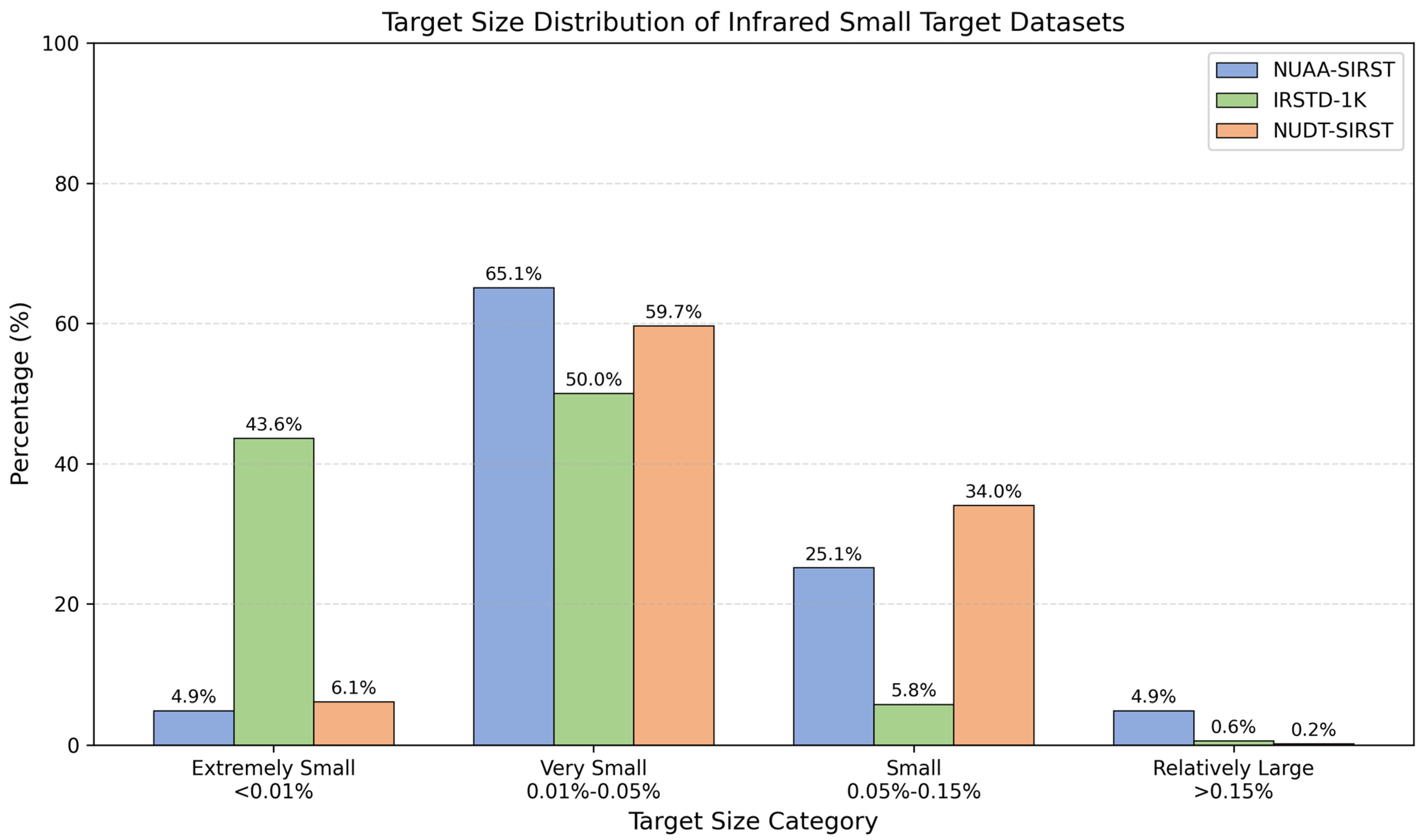
Figure 7.
Relative target-size distribution of the three IRSTD datasets. Target size is measured as the ratio between target area and image area, reflecting the scale differences among NUAA-SIRST, NUDT-SIRST, and IRSTD-1K.
Figure 7.
Relative target-size distribution of the three IRSTD datasets. Target size is measured as the ratio between target area and image area, reflecting the scale differences among NUAA-SIRST, NUDT-SIRST, and IRSTD-1K.
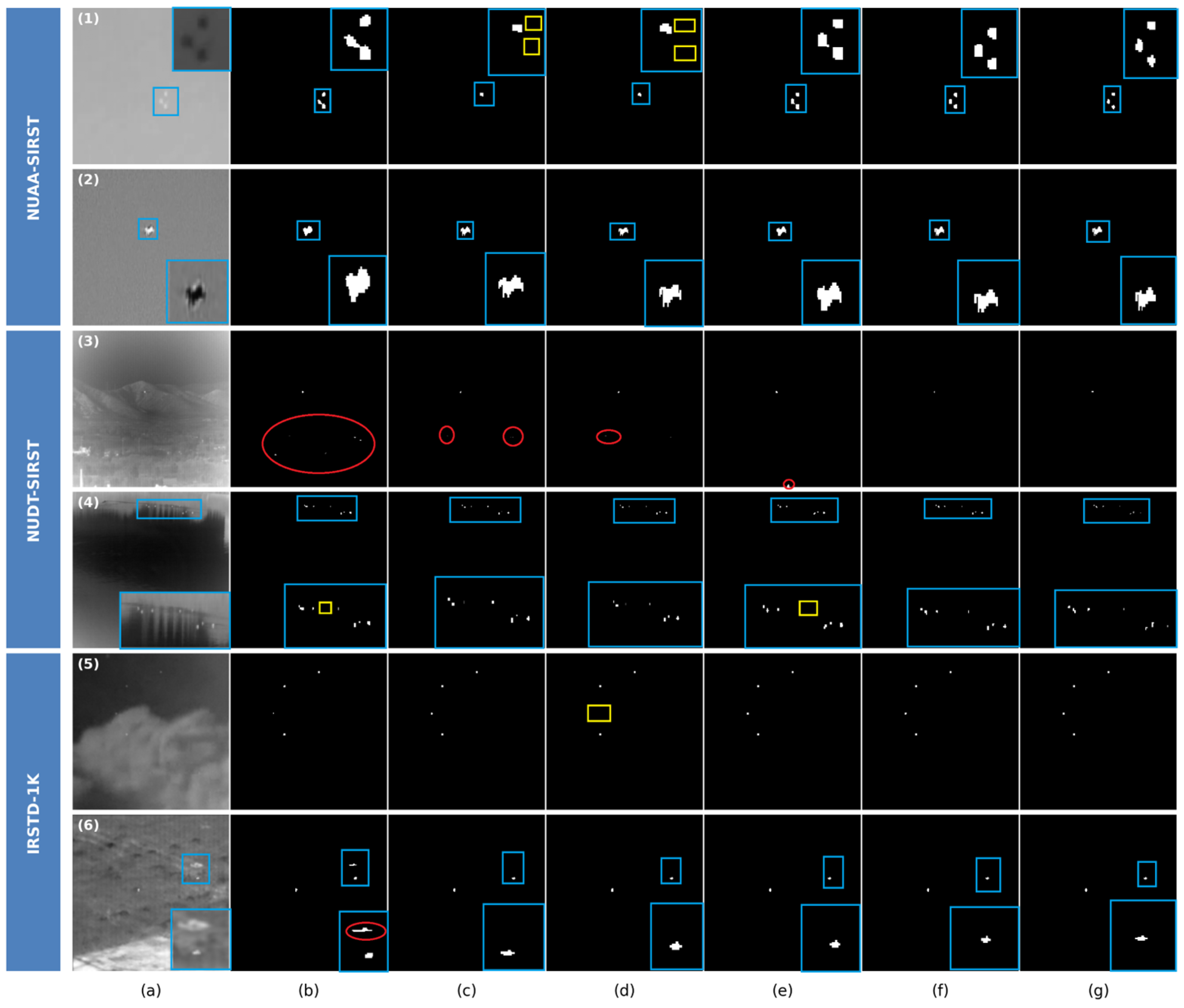
Figure 8.
Visual results obtained using different IRSTD methods on the NUAA-SIRST, NUDT-SIRST, and IRSTD-1K datasets. Blue, yellow, and red represent correctly detected targets, missed detections, and false positives, respectively. (a) Input. (b) ACMNet. (c) DNANet. (d) UIU-Net. (e) SCTransNet. (f) CFGMNet. (g) GT, ground truth.
Figure 8.
Visual results obtained using different IRSTD methods on the NUAA-SIRST, NUDT-SIRST, and IRSTD-1K datasets. Blue, yellow, and red represent correctly detected targets, missed detections, and false positives, respectively. (a) Input. (b) ACMNet. (c) DNANet. (d) UIU-Net. (e) SCTransNet. (f) CFGMNet. (g) GT, ground truth.
Figure 9.
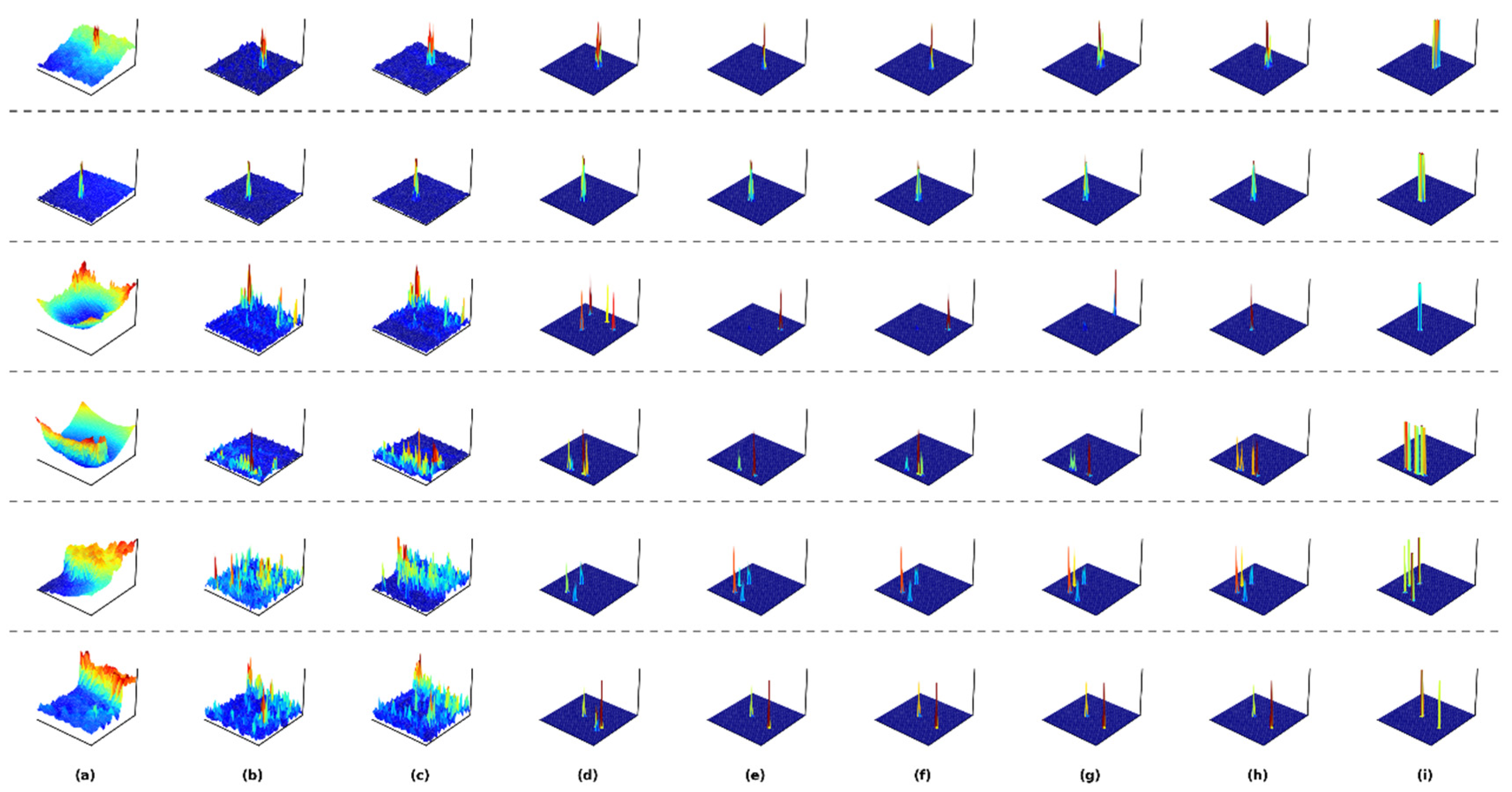
3D visualization of saliency maps generated by different methods on six test images. (a) Input. (b) Top-Hat. (c) TLLCM. (d) ACM. (e) DNANet. (f) UIU-Net. (g) SCTransNet. (h) CFGMNet. (i) GT, ground truth.
Figure 9.
3D visualization of saliency maps generated by different methods on six test images. (a) Input. (b) Top-Hat. (c) TLLCM. (d) ACM. (e) DNANet. (f) UIU-Net. (g) SCTransNet. (h) CFGMNet. (i) GT, ground truth.
Figure 10.
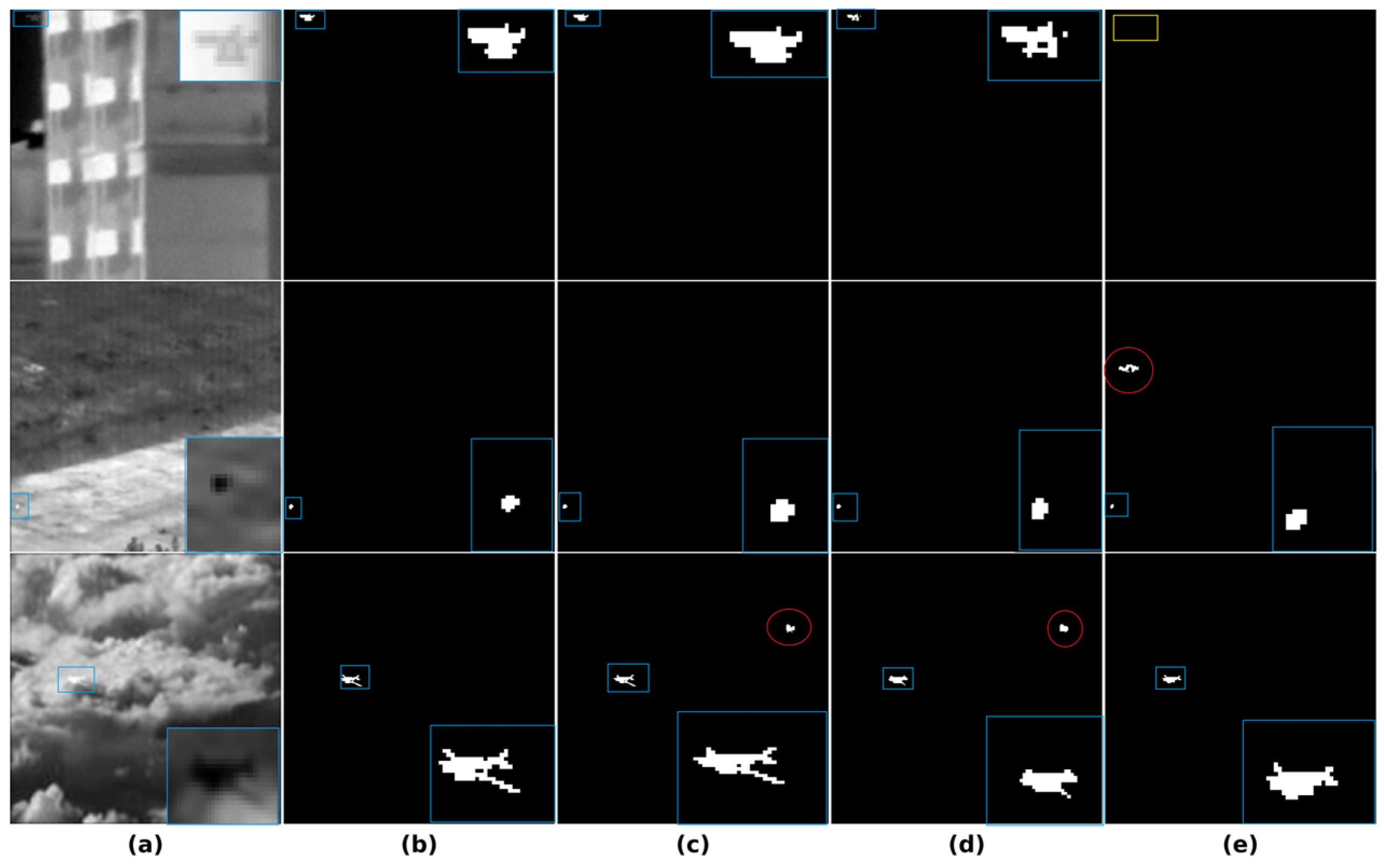
Representative failure cases on the NUDT-SIRST dataset, including blurred target boundaries, substantial target-scale variation, and weak target–background frequency differences. (a) Input image. (b) Ground truth. (c) SCTransNet. (d) UIU-Net. (e) CFGMNet.
Figure 10.
Representative failure cases on the NUDT-SIRST dataset, including blurred target boundaries, substantial target-scale variation, and weak target–background frequency differences. (a) Input image. (b) Ground truth. (c) SCTransNet. (d) UIU-Net. (e) CFGMNet.
Figure 11.
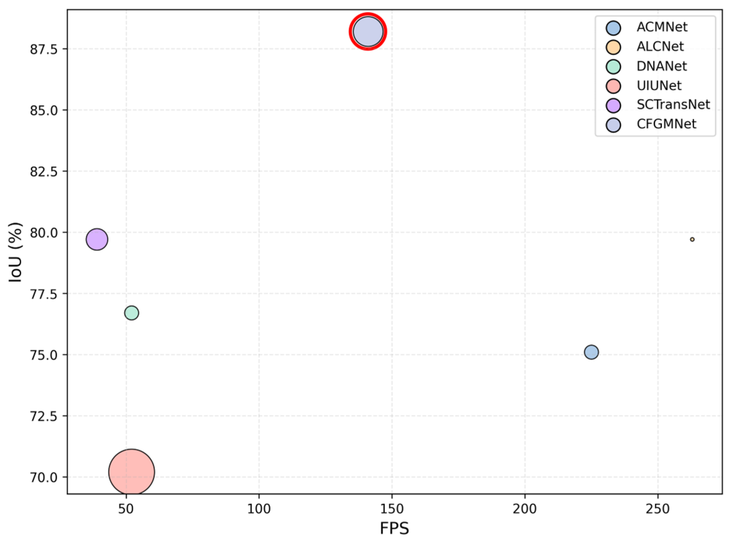
Comparison of the accuracy-speed trade-off among different methods. The red square represents the proposed CFGMNet, which achieves a favorable balance between detection accuracy and inference speed.
Figure 11.
Comparison of the accuracy-speed trade-off among different methods. The red square represents the proposed CFGMNet, which achieves a favorable balance between detection accuracy and inference speed.
Figure 12.
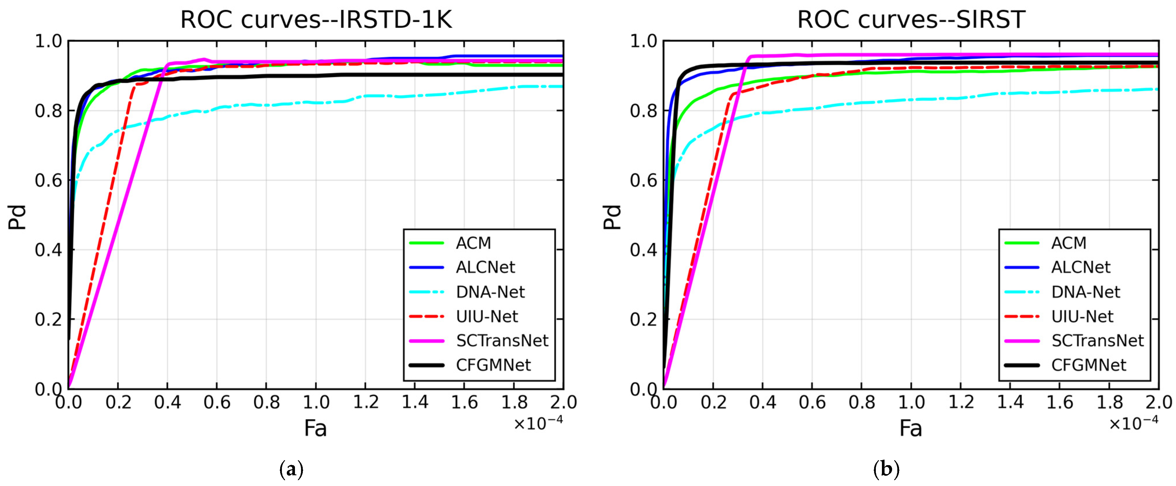
ROC curves of all compared methods on two infrared small target detection datasets. (a) ROC curves on the IRSTD-1K dataset, which compares the detection probability (Pd) against false alarm rate (Fa) across different methods; (b) ROC curves on the SIRST-3 dataset, presenting the corresponding Pd-Fa performance comparison of all involved algorithms.
Figure 12.
ROC curves of all compared methods on two infrared small target detection datasets. (a) ROC curves on the IRSTD-1K dataset, which compares the detection probability (Pd) against false alarm rate (Fa) across different methods; (b) ROC curves on the SIRST-3 dataset, presenting the corresponding Pd-Fa performance comparison of all involved algorithms.
Figure 13.
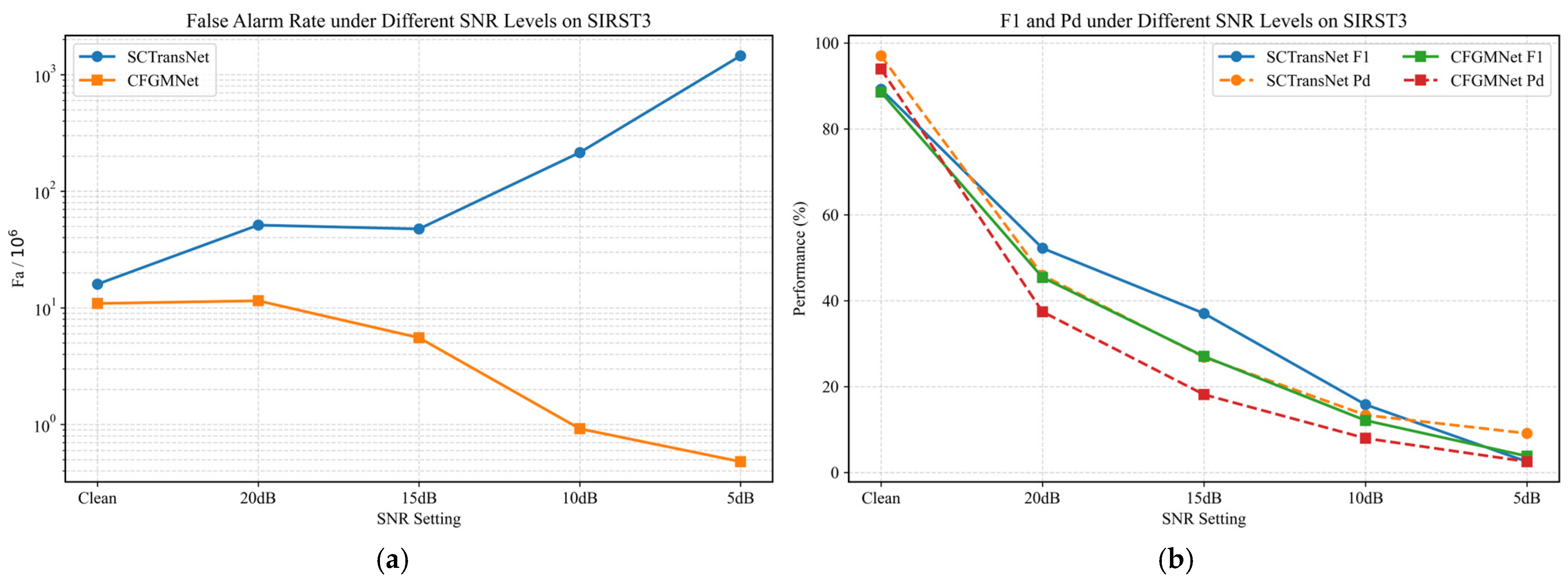
Robustness analysis under different SNR conditions on the SIRST3 dataset. (a) Trends of F1 and Pd. (b) Trend of Fa. Since Fa values vary greatly across different noise levels, the vertical axis in (b) is shown on a logarithmic scale.
Figure 13.
Robustness analysis under different SNR conditions on the SIRST3 dataset. (a) Trends of F1 and Pd. (b) Trend of Fa. Since Fa values vary greatly across different noise levels, the vertical axis in (b) is shown on a logarithmic scale.
Figure 14.
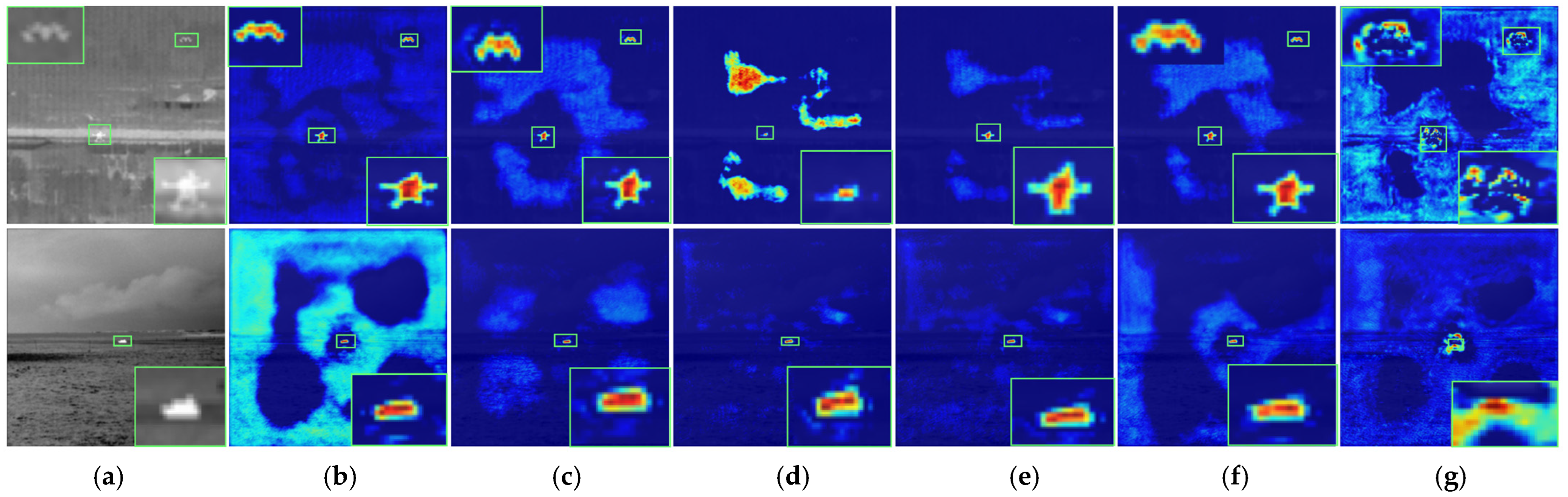
Visualization of the mid-layer feature responses for different ablation variants (a) shows the original image; (b) shows the full CFGMNet; (c–g) show the response results after removing the bottleneck layer CFG, X4CFG, LCG, AG + CA, and DH, respectively.
Figure 14.
Visualization of the mid-layer feature responses for different ablation variants (a) shows the original image; (b) shows the full CFGMNet; (c–g) show the response results after removing the bottleneck layer CFG, X4CFG, LCG, AG + CA, and DH, respectively.
Table 1.
Conceptual comparison between CFGMNet and representative IRSTD methods. The comparison focuses on backbone type, core idea, and the key methodological difference from CFGMNet.
Table 1.
Conceptual comparison between CFGMNet and representative IRSTD methods. The comparison focuses on backbone type, core idea, and the key methodological difference from CFGMNet.
| Method | Backbone Type | Core Idea | Key Difference from CFGMNet |
|---|
| SCTransNet | Transformer | Spatial–channel attention | No explicit frequency decomposition |
| MiM-ISTD | Mamba | Global–local Mamba modeling | Lacks background-constrained verification |
| IRMamba | Mamba | Difference-enhanced Mamba | No structured frequency gating |
| SAMamba | Mamba | Hierarchical state-space fusion | No low/high-frequency separation |
| EAMNet | Mamba-based | Feature enhancement | Weak false-alarm suppression |
| CFGMNet | Mamba-CNN hybrid | Frequency-guided modeling with background-aware gating | Explicit low–high frequency decomposition with background-aware gated verification |
Table 2.
Quantitative comparison with representative IRSTD methods on three benchmark datasets. Pd, F1, mIoU, and nIoU are reported in %, while Fa is reported in ×10−6. ↑/↓ indicates that higher/lower values are better. Bold and underline denote the best and second-best results, respectively.
Table 2.
Quantitative comparison with representative IRSTD methods on three benchmark datasets. Pd, F1, mIoU, and nIoU are reported in %, while Fa is reported in ×10−6. ↑/↓ indicates that higher/lower values are better. Bold and underline denote the best and second-best results, respectively.
| Method | NUAA-SIRST | NUDT-SIRST | IRSTD-1K |
|---|
| Pd ↑ | Fa ↓ | F1 ↑ | mIoU | nIoU | Pd ↑ | Fa ↓ | F1 | mIoU | nIoU | Pd ↑ | Fa ↓ | F1 ↑ | mIoU | nIoU |
|---|
| Top-Hat [6] | 79.84 | 1012 | 14.63 | 7.14 | 18.27 | 78.41 | 166.7 | 33.52 | 20.72 | 28.98 | 75.11 | 1432 | 16.02 | 10.06 | 7.438 |
| TLLCM [7] | 79.09 | 5899 | 5.00 | 1.03 | 4.10 | 62.01 | 1608 | 7.23 | 2.18 | 4.32 | 77.39 | 6738 | 2.19 | 3.31 | 0.78 |
| Max-Median [10] | 69.20 | 55.33 | 10.67 | 4.17 | 12.31 | 58.41 | 36.89 | 7.64 | 4.20 | 3.67 | 65.21 | 59.73 | 8.15 | 7.00 | 3.05 |
| WSLCM [8] | 77.95 | 5446 | 4.81 | 1.16 | 6.84 | 56.82 | 1309 | 5.99 | 2.28 | 3.87 | 72.44 | 6619 | 2.13 | 3.45 | 0.68 |
| ACM [12] | 90.63 | 16.23 | 80.87 | 68.02 | 68.67 | 91.64 | 58.71 | 76.40 | 61.81 | 66.25 | 92.49 | 56.07 | 74.25 | 62.17 | 58.18 |
| ALCNet [15] | 93.20 | 39.15 | 83.92 | 71.53 | 70.25 | 93.35 | 37.42 | 79.60 | 65.83 | 69.20 | 92.25 | 59.80 | 75.75 | 61.28 | 56.14 |
| DNANet [13] | 94.50 | 9.78 | 86.83 | 76.73 | 80.52 | 96.61 | 9.87 | 92.14 | 87.74 | 89.74 | 90.92 | 13.72 | 78.62 | 63.42 | 65.71 |
| UIU-Net [14] | 95.74 | 15.86 | 86.93 | 76.58 | 78.93 | 98.79 | 10.79 | 96.29 | 93.84 | 93.81 | 93.23 | 22.70 | 76.67 | 64.99 | 65.81 |
| SCTransNet [4] | 97.24 | 14.67 | 89.10 | 80.32 | 83.60 | 98.51 | 4.29 | 96.95 | 94.21 | 94.23 | 92.27 | 10.74 | 79.72 | 66.30 | 66.39 |
| EAMNet [27] | 96.25 | 4.94 | 83.69 | 76.28 | 74.59 | 90.62 | 26.14 | 79.52 | 65.32 | 70.28 | 90.91 | 27.05 | 75.36 | 63.28 | 57.13 |
| CFGMNet | 99.08 | 5.98 | 93.77 | 85.27 | 86.09 | 95.87 | 9.32 | 94.29 | 89.18 | 90.02 | 88.89 | 9.11 | 79.83 | 66.62 | 67.02 |
Table 3.
Statistical stability analysis of CFGMNet under different random seeds. Results are reported as mean ± standard deviation over three independent runs with seeds 42, 123, and 456. Best results are not cherry-picked. All experiments follow identical training settings. ↑ and ↓ indicate that higher values and lower values are better, respectively.
Table 3.
Statistical stability analysis of CFGMNet under different random seeds. Results are reported as mean ± standard deviation over three independent runs with seeds 42, 123, and 456. Best results are not cherry-picked. All experiments follow identical training settings. ↑ and ↓ indicate that higher values and lower values are better, respectively.
| Metric | SIRST3 | NUAA-SIRST | NUDT-SIRST | IRSTD-1K |
|---|
| mIoU (%) ↑ | 79.38 ± 0.22 | 85.25 ± 0.90 | 89.23 ± 0.06 | 66.48 ± 0.12 |
| nIoU (%) ↑ | 82.64 ± 0.19 | 86.37 ± 1.14 | 90.02 ± 0.08 | 67.39 ± 0.50 |
| Pd (%) ↑ | 94.48 ± 0.47 | 99.69 ± 0.53 | 95.94 ± 0.42 | 90.69 ± 1.59 |
| Fa (×10−6) ↓ | 11.86 ± 0.82 | 5.86 ± 0.20 | 9.49 ± 0.15 | 9.14 ± 1.22 |
| F1 (%) ↑ | 88.52 ± 0.14 | 93.19 ± 0.53 | 94.12 ± 0.29 | 79.34 ± 0.42 |
Table 4.
Comparison of model complexity, accuracy, and inference speed on NUAA-SIRST. Parameters are reported in M, FLOPs in G, mIoU in %, and FPS under the same forward-pass-only evaluation protocol.
Table 4.
Comparison of model complexity, accuracy, and inference speed on NUAA-SIRST. Parameters are reported in M, FLOPs in G, mIoU in %, and FPS under the same forward-pass-only evaluation protocol.
| Method | Type | Param (M) | FLOPs (G) | mIoU | FPS |
|---|
| ACMNet | CNN | 0.52 | 1.01 | 68.02 | 232 |
| DNANet | CNN | 4.7 | 28.56 | 76.73 | 16 |
| ABCNet | CNN + ViT | 106.99 | 166.27 | 81.01 | 18 |
| SCTransNet | CNN + ViT | 11.19 | 10.17 | 80.32 | 39 |
| CFGMNet | CNN + Mamba | 21.4 | 36.5 | 85.27 | 141 |
Table 5.
Robustness comparison under different SNR conditions on SIRST3. Clean denotes original test images without added Gaussian noise. F1 and Pd are reported in %, while Fa is reported in ×10−6.
Table 5.
Robustness comparison under different SNR conditions on SIRST3. Clean denotes original test images without added Gaussian noise. F1 and Pd are reported in %, while Fa is reported in ×10−6.
| Model | Setting | F1 | Pd | Fa |
|---|
| SCTransNet | Clean | 89.21 | 97.01 | 15.98 |
| CFGMNet | Clean | 88.57 | 93.95 | 10.91 |
| SCTransNet | 20 dB | 52.21 | 45.91 | 51.28 |
| CFGMNet | 20 dB | 45.41 | 37.41 | 11.51 |
| SCTransNet | 15 dB | 37.03 | 26.84 | 47.52 |
| CFGMNet | 15 dB | 27.02 | 18.14 | 5.55 |
| SCTransNet | 10 dB | 15.80 | 13.36 | 214.94 |
| CFGMNet | 10 dB | 12.12 | 7.97 | 0.92 |
| SCTransNet | 5 dB | 2.51 | 9.10 | 1451.77 |
| CFGMNet | 5 dB | 3.80 | 2.52 | 0.48 |
Table 6.
Structural ablation study. CFG denotes the CFG-Mamba module at the bottleneck stage, X4CFG denotes the CFG-Mamba module inserted after the fourth encoder stage, LCG denotes the Local Contrast Gate, AG denotes the spatial attention gate, CA denotes channel attention, and DH denotes the decoupled prediction head. ✔ denotes the module is adopted, and × denotes the module is removed.
Table 6.
Structural ablation study. CFG denotes the CFG-Mamba module at the bottleneck stage, X4CFG denotes the CFG-Mamba module inserted after the fourth encoder stage, LCG denotes the Local Contrast Gate, AG denotes the spatial attention gate, CA denotes channel attention, and DH denotes the decoupled prediction head. ✔ denotes the module is adopted, and × denotes the module is removed.
| Method | CFG | X4CFG | LCG | AG | CA | DH | mIoU | nIoU | Pd | Fa |
|---|
| Baseline | × | × | × | × | × | × | 69.34 | 69.17 | 96.33 | 32.08 |
| I | ✔ | × | × | × | × | × | 75.30 | 77.26 | 97.25 | 15.03 |
| II | ✔ | ✔ | × | × | × | × | 78.46 | 79.17 | 97.25 | 13.95 |
| III | ✔ | ✔ | ✔ | × | × | × | 79.28 | 82.24 | 99.08 | 10.29 |
| IV | ✔ | ✔ | ✔ | ✔ | ✔ | × | 82.53 | 84.25 | 99.08 | 7.62 |
| Full model | ✔ | ✔ | ✔ | ✔ | ✔ | ✔ | 85.27 | 86.09 | 99.08 | 5.98 |
Table 7.
Loss function ablation study. ✔ denotes the module is adopted, and × denotes the module is removed. Bold values indicate the best results, and underlined values indicate the second-best results.
Table 7.
Loss function ablation study. ✔ denotes the module is adopted, and × denotes the module is removed. Bold values indicate the best results, and underlined values indicate the second-best results.
| BCE | Dice | OHEM | Focal | Pd | Fa | mIoU |
|---|
| ✔ | × | × | × | 98.17 | 5.11 | 74.08 |
| ✔ | ✔ | × | × | 99.08 | 7.33 | 82.95 |
| ✔ | ✔ | ✔ | × | 99.08 | 6.82 | 84.07 |
| ✔ | ✔ | ✔ | ✔ | 99.08 | 5.98 | 85.27 |
Table 8.
Ablation study of LCG module with different receptive field sizes. Bold values indicate the best results, and underlined values indicate the second-best results.
Table 8.
Ablation study of LCG module with different receptive field sizes. Bold values indicate the best results, and underlined values indicate the second-best results.
| Method | Pd | Fa | mIoU |
|---|
| 3 × 3-LCG | 93.40 | 12.12 | 78.63 |
| 5 × 5-LCG | 93.95 | 10.35 | 79.48 |
| 7 × 7-LCG | 92.78 | 9.98 | 77.82 |
| Without LCG | 91.96 | 12.29 | 76.79 |
Table 9.
Performance comparison of different frequency decomposition strategies on the SIRST3 dataset. ↑ and ↓ indicate that higher values and lower values are better, respectively.
Table 9.
Performance comparison of different frequency decomposition strategies on the SIRST3 dataset. ↑ and ↓ indicate that higher values and lower values are better, respectively.
| Method | Pd ↑ | Fa ↓ | mIoU ↑ | F1 ↑ |
|---|
| 3 × 3 AvgPool | 93.95 | 10.35 | 79.43 | 88.57 |
| 5 × 5 AvgPool | 94.15 | 11.75 | 78.88 | 88.19 |
| 7 × 7 AvgPool | 93.89 | 12.51 | 78.88 | 88.19 |
| Gaussian (σ = 1.0) | 94.68 | 13.01 | 78.95 | 88.24 |
| Haar-LL | 93.36 | 12.52 | 78.04 | 87.67 |