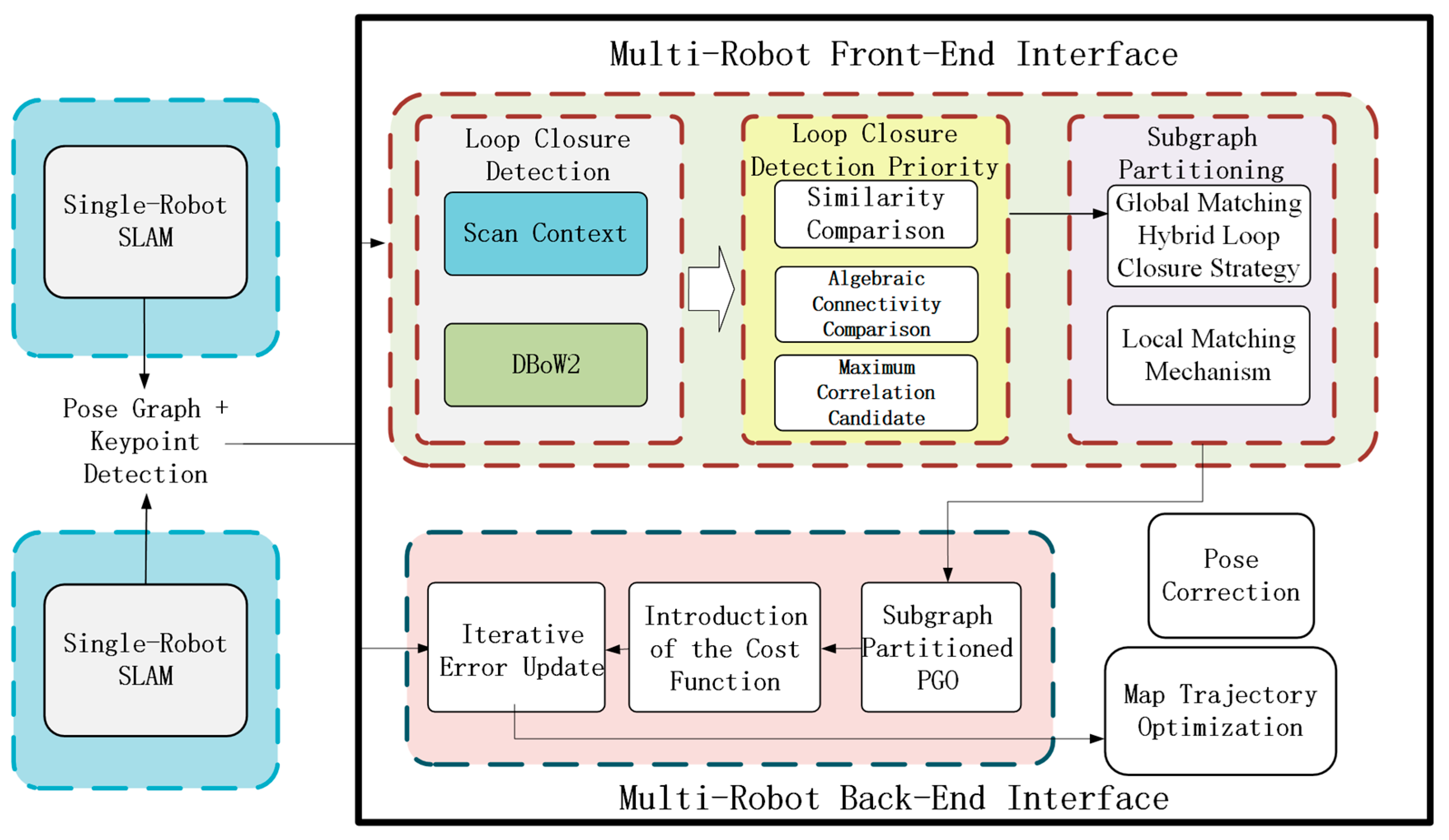
In the front-end of multi-robot collaborative SLAM systems, robots rely on transmitting keyframes to obtain relative poses. However, when computing loop closures, incorrect or loosely correlated loop frames are often introduced. This not only leads to the accumulation of errors in the robot’s pose estimation, causing the constructed map to deviate from the actual environment and impacting the system’s reliability and usability, but also consumes limited communication and computational resources. Therefore, this section proposes a loop closure detection algorithm under communication constraints based on maximizing algebraic connectivity. The algorithm utilizes the Laplacian matrix to select loop closures and applies a reasonable strategy to filter out correct loop closure edges while avoiding the processing of large amounts of redundant measurements. Additionally, subgraph partitioning is used to select the most connected loop closures for the robots, laying the foundation for multi-robot back-end pose graph optimization. The proposed algorithm integrates laser point clouds and visual features to perform cross-robot loop closure detection. The laser point cloud detection utilizes lidar to capture point cloud data, analyzing its features to identify environmental characteristics that assist in loop closure detection. The visual feature detection uses the camera to extract image feature points, representing them with descriptors and comparing the descriptors of image feature points at different times to detect loop closures. This multi-sensor fusion approach leverages the strengths of both lidar and cameras to enhance the accuracy of loop closure detection.
3.1.1. Global Matching Hybrid Loop Closure Strategy
In traditional global matching, greedy algorithms [
22] simply select the top A candidates with the highest similarity scores, where A is predefined by the user based on the robot’s communication and computational capacity. However, this approach may lead to candidate selections that are overly concentrated in high-similarity regions, resulting in redundancy. To address this issue, this section incorporates the concept of pose graph sparsification into the candidate prioritization process. By ranking candidate loop closure edges based on priority, the algorithm selects a subset of candidates that maximizes algebraic connectivity. This method ensures that the selected candidates are more evenly distributed across the pose graph, effectively reducing redundancy.
The multi-robot pose graph is defined to model the spatial relationships and measurement data among robots, and it is expressed as:
where
represents the set of vertices, with
denoting the number of robots.
corresponds to the set of pose vertices for the
th robot, where each vertex represents the robot’s pose at a specific time. These vertices encapsulate the observation information of robots at different time instances and serve as fundamental elements in constructing the pose graph. The set of edges
consists of two types of edges. The local edge set
represents intra-robot pose constraints, including odometry measurements and robot-specific loop closures. These edges capture the relative pose changes during a robot’s motion and its internal loop closures, which are crucial for maintaining the accuracy of local robot poses. The global edge set
consists of inter-robot loop closure candidate edges, representing potential loop closures between different robot poses. These edges are the primary focus of subsequent optimization.
To evaluate the algebraic connectivity of the pose graph, the rotated weighted Laplacian matrix is introduced as , where is the degree matrix and is the adjacency matrix. In multi-robot pose graph optimization, the adjacency matrix represents the direct connectivity relationships between robot poses, while the degree matrix reflects the connectivity degree of each robot pose. The Laplacian matrix integrates both pieces of information and is used to analyze the overall structure and stability of the pose graph.
The degree matrix
is an
diagonal matrix, where each diagonal element
represents the degree of vertex
, defined as the number of edges connected to vertex
. It is expressed as:
In the multi-robot pose graph, represents the number of relative pose constraints between robot and the poses of other robots. A larger indicates that the robot has interactions with a greater number of other robots within the multi-robot system.
The adjacency matrix
is also an
matrix used to describe the connectivity relationships between vertices in the graph:
Specifically, when , , indicating that a robot’s pose does not form a relative pose constraint with itself. When , if there is an edge connecting vertices and , then , meaning that a relative pose constraint exists between the poses of robot and robot in the multi-robot pose graph. Conversely, if there is no edge between vertices and , then , indicating that there is no direct relative pose constraint between the poses of robot and robot in the current graph representation.
The definition of the Laplacian matrix
is closely related to the structure of the pose graph. Its elements
are defined based on the vertices and edges in the pose graph as follows:
When , the Laplacian matrix element is defined as , where represents the set of edges connected to vertex . In the multi-robot pose graph, vertex corresponds to a robot’s pose at a specific time. This equation indicates that the diagonal elements of the Laplacian matrix are the sum of the weights of all edges connected to vertex .
When , the Laplacian matrix element is defined as , where indicates that there is an edge between vertices and , and represents the weight of this edge. In the multi-robot pose graph, edges represent relationships between robot poses. For example, if loop closure detection identifies an association between the poses of two robots at different locations, an edge is added between the corresponding vertices.
When , the Laplacian matrix element is defined as , indicating that there is no direct edge between vertices and . In the multi-robot pose graph, if loop closure is not detected between the poses of two robots, the corresponding element in the Laplacian matrix remains zero, signifying the absence of a direct connection.
Next, we determine the edge weights. For , the weight is set to 1. This is because these edges represent fixed measurement constraints within a single robot, where the constraints between adjacent poses are relatively certain. Assigning a fixed weight to these edges is crucial for maintaining the fundamental structure and connectivity of the pose graph, helping to stabilize its foundational framework.
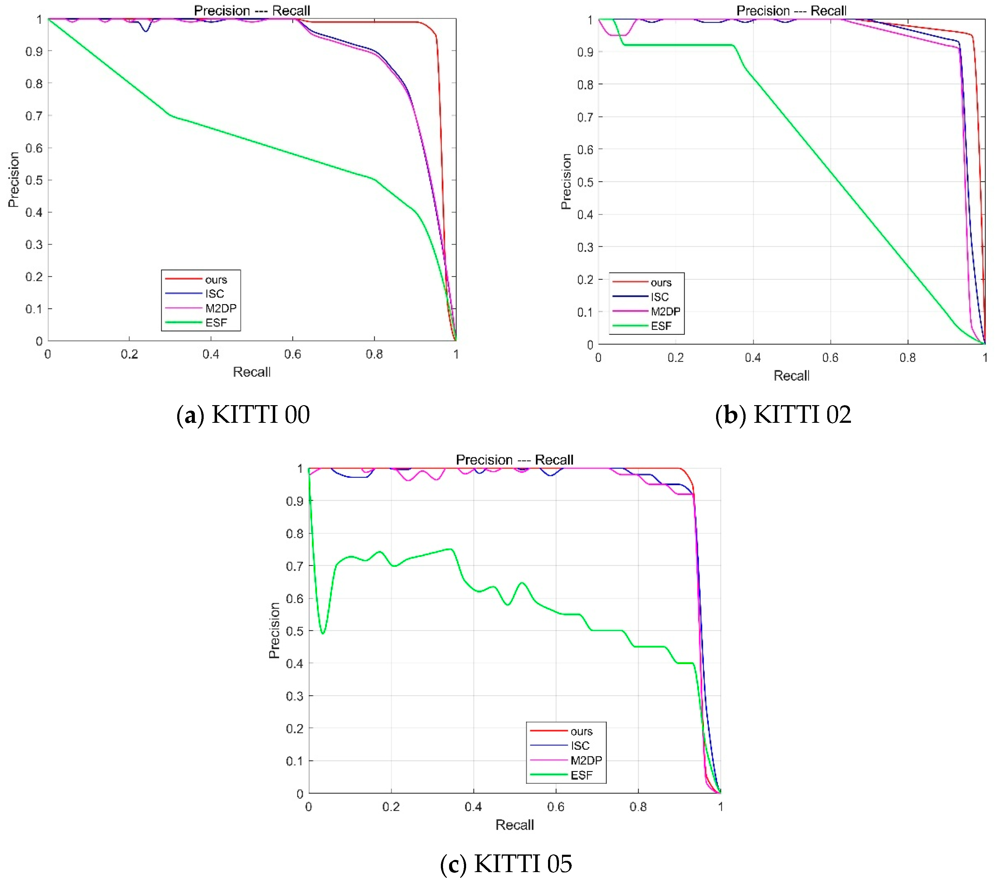
For
, the similarity between edges is computed using the Scan Context [
28] LiDAR loop closure detection algorithm, and the bags of binary words for fast place recognition in image sequences (DBoW2) [
29] visual loop closure detection algorithm. Equations (5) and (6), respectively, represent the similarity calculation formulas for LiDAR-based and vision-based loop closure detection:
In this formula,
and
represent two different LiDAR scan frames, while
denotes the number of angular bins used to partition the scan data for statistical analysis and computation. The feature value in the
-th angular bin of the query scan
is represented by
, whereas
corresponds to the feature value in the same angular bin of the reference scan
. The norms
and
are used for vector normalization. This formula quantifies the similarity between two scan frames by assessing the differences in their feature values across corresponding angular bins. If the comparison score is less than the set threshold
(which is 0.1 in this paper), a loop closure is detected, and its similarity is recorded for subsequent weight calculation. If the comparison score exceeds the set threshold, it is treated as a false loop closure.
Here, and represent two different visual word vectors, while and denote the weight of the -th visual word in image A and image B, respectively. The similarity between the two images is computed by comparing the differences in the intensity of their features. By finding the combination where the difference between the vector and is minimized, if the comparison score is less than the set threshold (0.25 in this paper), a loop closure is detected. The similarity is recorded for subsequent weight calculation, and if the comparison score exceeds the set threshold, it is treated as a false loop closure.
That is, the similarity obtained from LiDAR and visual loop closure is used to determine the edge weight , where , indicating that the weight of candidate loop closure edges is determined based on the global matching similarity score, which falls within the range of . For example, if the similarity score of the LiDAR or visual data scanned by two robots is 0.65, then is set to 0.65. This is because the reliability of candidate inter-robot loop closures largely depends on the degree of global matching similarity; the higher the similarity, the greater its potential value in constructing an accurate pose graph. By incorporating feature matching information into the pose graph structure evaluation, the system effectively enhances the accuracy of multi-robot localization and mapping.
Next, the enhanced pose graph Laplacian matrix is constructed:
where
is a binary variable used to determine the priority of candidate edge
. When
, it indicates that the candidate edge is selected for algebraic connectivity computation, meaning that the edge is considered to positively contribute to improving the overall quality of the pose graph. When
, the edge is excluded.
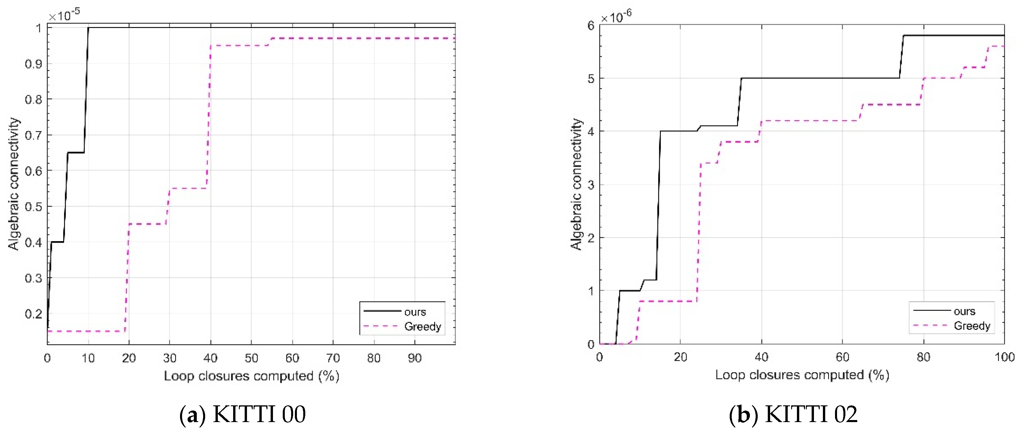
Finally, the algebraic connectivity of the pose graph is measured by computing the second smallest eigenvalue
of the rotationally weighted Laplacian matrix. The candidate subset is selected with the objective of maximizing
:
Through the above-mentioned algebraic connectivity-based filtering method, compared to selecting candidate edges solely based on similarity, the overall structure of the pose graph is considered more comprehensively. This effectively avoids selecting loop closure edges that, despite having high similarity, do not substantially contribute to the overall pose graph optimization and may even lead to incorrect closures. This ensures that the selected candidate edges are more aligned with the actual loop closure situations.
3.1.2. Local Matching Mechanism
Once the loop closure candidates are found, the system uses local features from sensors to accurately calculate the 3D relative position and orientation based on the type of sensor. Once the loop closure candidates are identified, the system uses local features obtained from sensors to calculate the 3D relative pose measurements based on the sensor type. To prevent redundant computations for the same loop closure and reduce communication overhead during geometric verification, a vertex coverage strategy is introduced. In situations where multiple robots are working together, if several loop closure candidates use the same vertex, only the necessary information about that shared vertex is sent, allowing for the quick calculations of all related position measurements.
Given
loop closure candidates with the corresponding vertex set
and edge set
, where an edge
represents a loop closure relationship connecting two vertices. The binary variable
is introduced, where
indicates that vertex
is selected for transmission, and
indicates that it is not transmitted. The objective is to minimize the number of selected vertices for transmission, which can be formulated as:
At the same time, the following constraint must be satisfied: for each edge
, at least one of the vertices must be selected for transmission, i.e.,
By solving this integer programming problem, the optimal vertex transmission scheme can be obtained. Using algorithms [
28,
29] to compute relative pose measurements, the results of different candidate edges based on common vertices are compared. If the relative pose differences calculated from multiple candidate edges are too large, it indicates that there may be erroneous loop closure edges among them. Through this vertex covering strategy, during multi-robot collaborative exploration in complex environments, data transmission can be significantly reduced, while effectively verifying the correctness of candidate loop closure edges.
By solving this integer programming problem, the optimal vertex transmission scheme can be obtained. This vertex coverage strategy significantly reduces data transmission volume when multiple robots collaborate to explore complex environments.
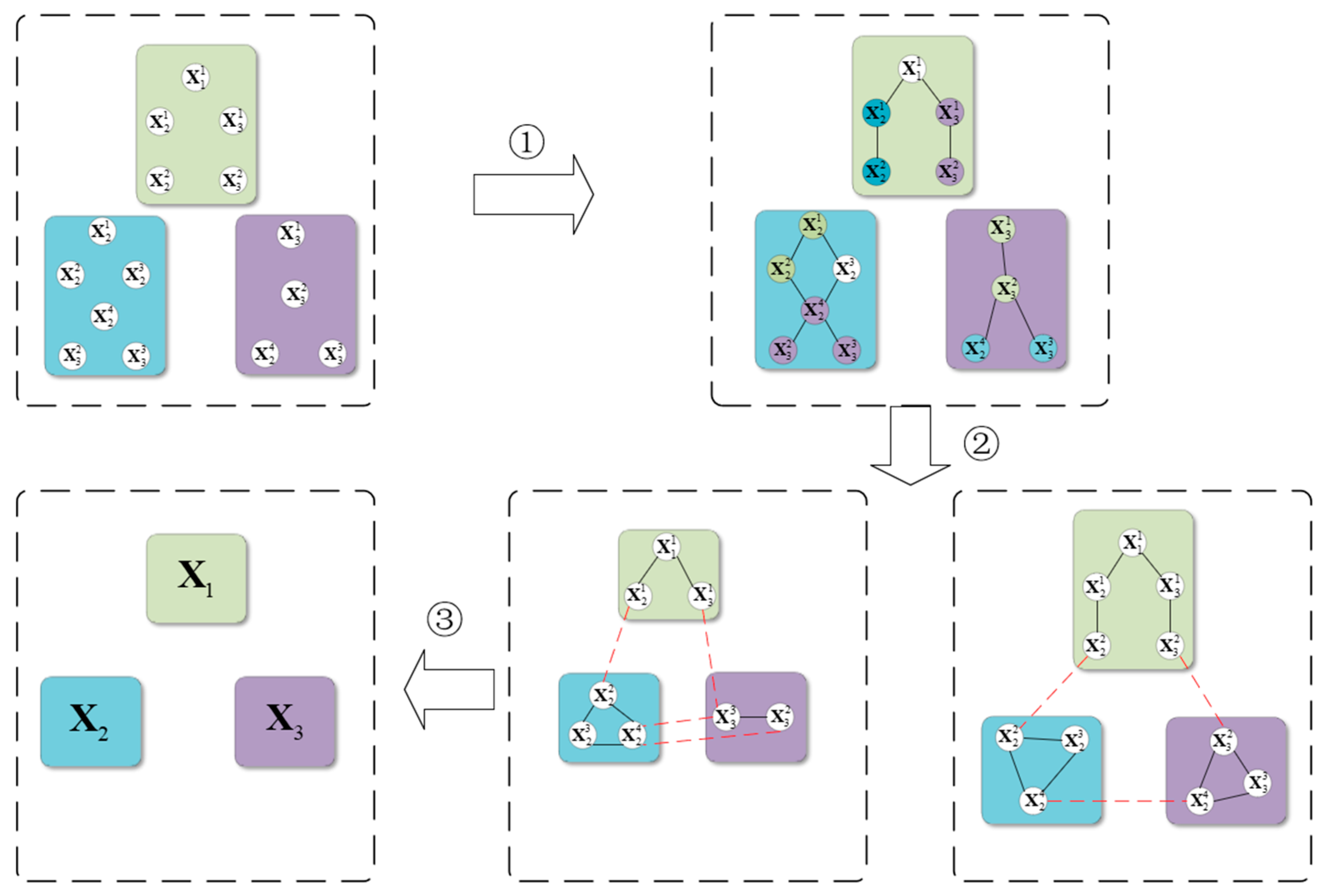
At the same time, the segmented subgraphs often exhibit imbalances, leading to excessive workloads for some robots while others remain underutilized. To address this issue, the subgraphs need to be fine-tuned by adjusting their scale to ensure a balanced distribution of variables and computational complexity. This process reduces cross-connections and redundancy within subgraphs, ultimately improving computational efficiency.
Let the segmented subgraphs be
, with the number of nodes in each subgraph represented as
. The mean and variance of the number of nodes in the subgraphs are computed as follows:
When balancing the subgraph partitioning, the criterion is the balance of the number of nodes and edges in each subgraph. Specifically, the variance of the number of nodes in each subgraph should not exceed 5% of the total number of nodes across all subgraphs. By continuously adjusting the subgraph partitioning scheme, nodes are moved from subgraphs with a larger number of nodes to those with fewer nodes, ensuring that the size of each subgraph becomes more balanced.


