Performance Evaluation and Calibration of Electromagnetic Field (EMF) Area Monitors Using a Multi-Wire Transverse Electromagnetic (MWTEM) Transmission Line

Abstract

The exposure levels generated by environmental electromagnetic field (EMF) sources can be measured and monitored by employing EMF area monitors. The operating spectrum of environmental EMF sources is not limited to high frequencies (f > 30 MHz) but also extends to low frequencies (f < 30 MHz), where sources associated, for example, with radio transmitters typically generate non-negligible field contributions. For this reason, professional EMF area monitors can be equipped with different field sensors, properly calibrated according to standardized procedures. Because low-frequency electric fields are very sensitive to environmental boundary conditions, equipping an EMF area monitor with electric field sensors, previously calibrated as stand-alone devices, can lead to measurement errors due to field perturbations introduced by the physical structure of the area monitor itself. This paper describes the activities carried out to assess the performance of an EMF area monitor in simulated realistic conditions and calibrate it in the 300 kHz–20 MHz frequency band. The activities were conducted using a multi-wire transverse electromagnetic (MWTEM) transmission line as a controlled electric field source, with dimensions suitable for exposure of the entire structure of the EMF area monitor. In view of using this approach to calibrate the area monitors as a whole instead of the individual sensors, the uniformity of the electric field generated by the available MWTEM transmission line was analyzed in detail both numerically and experimentally. Finally, the results of the evaluation and calibration of an area monitor are reported and discussed.

1. Introduction

The rapid and continuous growth of wireless communications and data transmissions requires a great number of stations that generate non-negligible environmental electromagnetic fields. This significantly increases the density of radiating sources while at the same time increasing public concerns about exposure levels to the electromagnetic fields generated by the necessary systems. Similarly, the massive use of wireless technologies in a great variety of equipment and the pervasive distribution of electrical power networks implies a large number of intentional and non-intentional sources of electromagnetic energy being distributed in the environment and operating in a very wide frequency range, ranging from tens of Hz to tens of GHz. In this highly complex electromagnetic scenario, exposure to electromagnetic fields is a topic of great importance, especially for people living near infrastructures recognized as EMF sources. Local authorities and government agencies have an interest in the real-time, continuous monitoring of the exposure levels generated by different sources to ensure that nearby areas comply with applicable national or international standards [1,2,3,4]. Typical areas of concern are schools, hospitals, and residential and public areas, not to mention exposure in the workplace. Classical electromagnetic field measurement instruments, despite their optimized performance and accuracy, are not suitable for this kind of task as they generally require the presence of an operator; in addition, due to limited autonomous power supplies and a lack of weatherproofing, they are not suitable for long-term or continuous unattended outdoor monitoring. These limitations have led to the development of EMF area monitors, i.e., electromagnetic field measurement systems that can autonomously measure field levels and record and transmit data. EMF area monitors are typically battery-operated and equipped with solar panels for an independent power supply. In general, an EMF area monitor can be fitted with a set of field probes covering all parts of the spectrum of interest for a particular site to be monitored. An example of an EMF area monitor in a real application scenario is shown in Figure 1.

By using an EMF area monitor, the measurements taken with a certain time step can be read remotely at any time or automatically sent at preset intervals to a remote PC or a data server via the mobile network. Alarms can be automatically sent to selected recipients if preset limits are exceeded. When measurements are required from several positions, an effective solution is to implement a geographically distributed network of EMF area monitors that can continuously detect exposure levels, present the results to the public in an easily accessible format, and compare the results with the applicable standards [1,2,3,4]. Several researchers, from both academia and industry, have investigated ways of satisfying the requirements set by the International Telecommunication Union (ITU) [5] for the monitoring of environmental electromagnetic fields. Various studies based on the integration of field probes with wireless sensor networks (WSNs) [6,7,8] or with radio interfaces based on the GSM/GPRS standard [9,10,11,12,13,14] can be found in the literature. Recently, as described in [15], extensive geographical monitoring has been experimented by integrating an area monitor inside a car. The constant and current interest in the topic is demonstrated by the publication of scientific and technical papers, even in recent years [16,17,18,19,20]. In this framework, considering that an EMF area monitor is a more complex measuring system than a classical EMF probe and considering that it can operate in scenarios with different electrical boundary conditions (e.g., with or without cabling and a power supply unit for connection to the mains), researchers have studied the device’s behavior in different simulated environments [21].

In this paper, a description of the architecture of a typical EMF area monitor is followed by a presentation of the activities carried out in order to calibrate it as a whole system and validate its behavior. To this end, the electric field generated by a multi-wire TEM (MWTEM) transmission line was analyzed in detail both numerically and experimentally in order to evaluate its capability to generate controlled electric field distributions that are sufficiently uniform for the exposure of the entire structure of the EMF area monitor for frequencies up to 30 MHz.

In most cases, sources capable of generating non-negligible field contributions are associated with mobile phone systems or radio transmitters operating at frequencies higher than 30 MHz. However, in certain cases—often involving high emission levels—high-power RF sources operating at frequencies below 30 MHz are used for long-distance communication transmitters (e.g., for naval or military communications) or for industrial, scientific, and medical (ISM) applications, authorized by the ITU, such as dielectric heating, plastic welding, food processing, and short-wave diathermy.

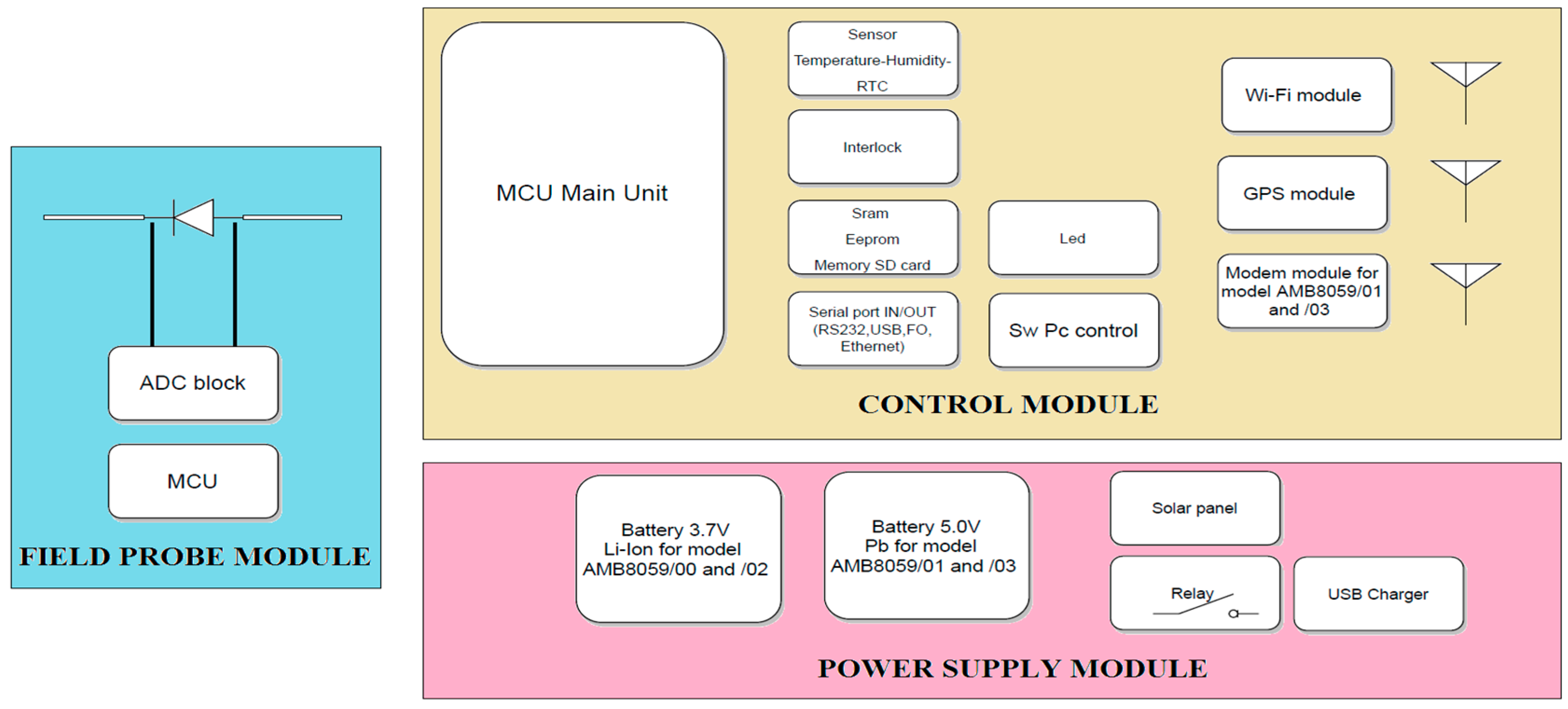
2. The Structure of an EMF Area Monitor

Figure 2 presents the general structure of the AMB-8059 area monitor. Three orthogonal broadband probes in the field probe module measure the field amplitude, and the resulting signal is converted by the analog to digital converter (ADC) and sent to the micro-controller unit (MCU). The area monitor, managed by the control module, is able to autonomously perform, acquire, memorize, and transmit measurements. The area monitor is equipped with a set of radio interfaces (Wi-Fi, GSM/GPRS, LTE) necessary for remote control and data exchange. The power supply module optimizes power consumption for long-time autonomous operation by managing battery use and charging via solar panel or, if available, via a power supply unit connected to the mains. Due to its non-negligible structure and the use of cables, the presence of an area monitor can modify the field under measurement, causing errors in the measurement results. This issue is magnified for frequencies below 30 MHz, as analyzed in [22] for electric field measurement with a rod antenna. To solve this kind of problem, the AMB-8059 is equipped with a relay that automatically disconnects the electrical connection when not needed. For the same reason, to improve measurement accuracy, the calibration of the area monitor has to be reconsidered as a whole system, as typically the field probes are calibrated as stand-alone devices and the effects of integrating them within the area monitor have to be evaluated and, if necessary, taken into account.

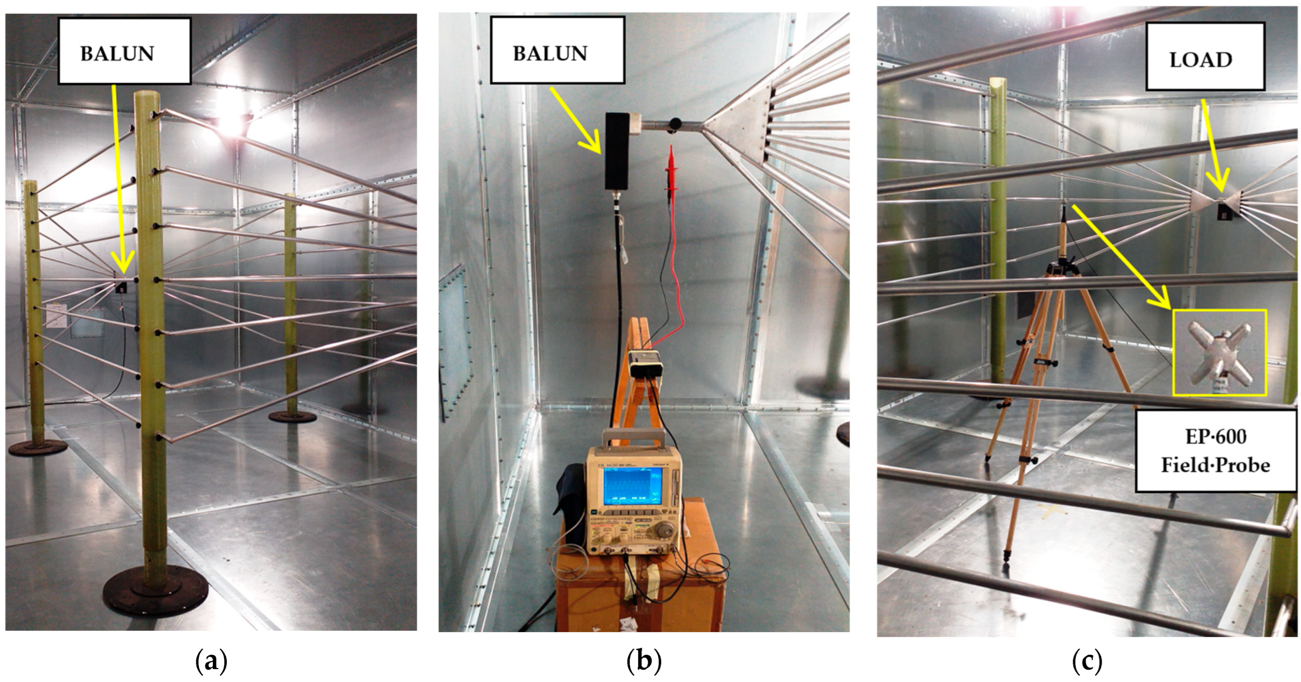
3. Experimental Setup

To calibrate and evaluate the performance of an area monitor as a whole system, we need to generate a controlled and sufficiently uniform electric field in a volume suitable for hosting the entire structure of the device under calibration. At higher frequencies (f > 30 MHz), this is easily accomplished by means of standard radiating devices like simple dipoles, biconical, log-periodic, and horn antennas. The same approach cannot be used at lower frequencies (f < 30 MHz), as in this frequency range, the physical size of dipolar antennas becomes impractical, and in order to operate under realistic electromagnetic field conditions, it is necessary to stay far from the antenna itself. This implies an overly challenging test setup while requiring the generation of intense electromagnetic fields over a large area.

A possible approach for the generation of high field levels in a confined region while avoiding conventional antennas is based on the use of transverse electromagnetic (TEM) transmission lines that in the enclosed volume support a uniform and linearly polarized plane wave [23,24,25].

Each transmission line composed of two separate conductors for f < f_C1 can support the propagation of the TEM field configuration, while for f > f_C1, other field configurations associated with high-order modes (f_C1 being the cut-off frequency of the first high-order mode) can occur and heavily modify the field configuration. The main properties of a TEM wave are that the electric and magnetic fields are perpendicular to each other and both are transverse to the wave direction of propagation. This type of wave, known as a plane wave, is also present in the far field of an antenna radiating in free space. Coaxial lines, parallel plate lines, TEM cells, and similar structures (all characterized by the presence of two separate conductors or groups of conductors) can support this field configuration. For this reason, they are widely used to generate uniform fields for electromagnetic compatibility testing [26,27] and calibration. Wire array cells belong to this category, and thus, the multi-wire TEM line has been evaluated and validated for calibration activities.

Because classical TEM cells generally have small dimensions and a closed structure, it is very difficult to insert an entire area monitor inside their useful volume. They are therefore a good solution for calibrating smaller instruments like classical field probes, but impractical for equipment as large as an area monitor.

An adequately sized alternative structure, composed of wire arrays and capable of supporting a TEM mode, is the multi-wire TEM (MWTEM) transmission line [28]. This device is less popular than TEM cells and, to the best of the authors’ knowledge, has never been used for the calibration and validation of field probes. The structure of the MWTEM line used for the activities described in this paper is shown in Figure 3, where three different sections can be observed: a central uniform multi-conductor transmission line enclosing the volume used for testing, and two lateral tapered transmission lines. At one end (the input port), the MWTEM line is equipped with a balun/matching network (50 Ω/200 Ω) and at the other end with a 200 Ω dummy load. The balun is necessary as no metallic element of the line supporting the TEM wave is connected to a constant potential (the device operates in balanced mode). The MWTEM line is equipped with a nominal 200 Ω load as this matches its characteristic impedance; according to transmission line theory, this is the optimal choice for minimizing reflections from the load and reducing standing wave phenomena along the line in the higher frequency band.

As shown in Figure 3, instead of metallic plates (as in classical TEM structures, e.g., the parallel plate line [26]), the two halves of the line are composed of an array of seven aluminum pipes (2 cm in diameter). These pipes are parallel in the central section and taper between the central section and the two ends. The MWTEM line used for experiments is pictured in Figure 4. In particular, Figure 4b,c show the two ends of the line with the balun and the load, respectively.

The use of a TEM cell composed of wire arrays instead of planar elements greatly complexifies the electromagnetic problem to be solved in order to find the electrical parameters of the device and accurately analyze the uniformity of the generated electric field. Because no analytical formula is available for the field values and characteristic impedance, a simulation software has been used to obtain a detailed and accurate characterization of the device. The results of the characterization by numerical simulation are reported and discussed in Section 4.

An outline of the theory of MWTEM cells is reported in Appendix A. Starting from the description of the TEM mode field components existing in the basic structure of the parallel plate line, an approximated theory of the TEM mode valid for an MWTEM in a quasi-static condition is reported. The relationships obtained according to the quasi-static model can be profitably employed for the design of a generic N-wire MWTEM line in terms of transversal electric field components and line impedance.

The MWTEM transmission line is an open structure, so when driven by radiofrequency power, it can radiate non-negligible fields in the surrounding area. During the experimental activities, it was driven using a 75 W power amplifier, then placed inside a shielded chamber to minimize interference with sensitive equipment in the nearby area. The technical characteristics of all equipment used during the experiments are summarized in

Table 1. Characteristics of equipment used for the experimental activities.

Equipment	Manufacturer	Model	Characteristics
Shielded Chamber	Beltech	-	Dimensions: 6.1 × 4.9 × 3.6 m
MWTEM	Comtest	-	7 + 7 wires balanced transm. line, 4.5 × 2.3 × 1.5 m, Z0 = 200 Ω, fmax = 20 MHz
MWTEM Balun	Comtest	-	Impedances levels: 50 Ω /200 Ω
MWTEM Load	Comtest	-	Impedance: 200 Ω (nominal value)
RF Signal Generator	Hewlett Packard	E4400B	Freq. band: 250 kHz–1 GHz
Power Amplifier	Amplifier Research	75A250	Freq. band: 10 kHz–250 MHz, Pmax = 75 W
Digital Oscilloscope	Yokogawa	DL1620	fmax = 200 MHz
High Voltage Diff. Probe	Sapphire Instruments	SI-9010	Vmax = ±7000 V, fmax = 70 MHz
Electric Field Probe	Narda STS	EP600	Freq. band: 100 kHz–9.25 GHz, 0.14–140 V/m
Network Analyzer	Agilent	E5061B	Freq. band: 5 Hz–3 GHz

.

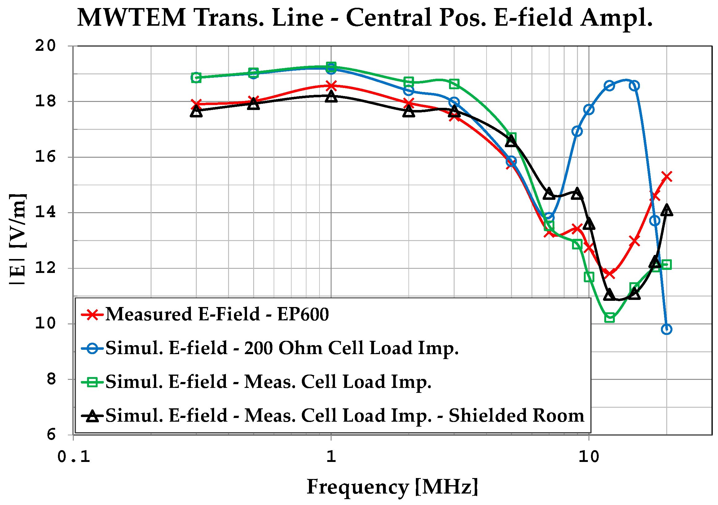
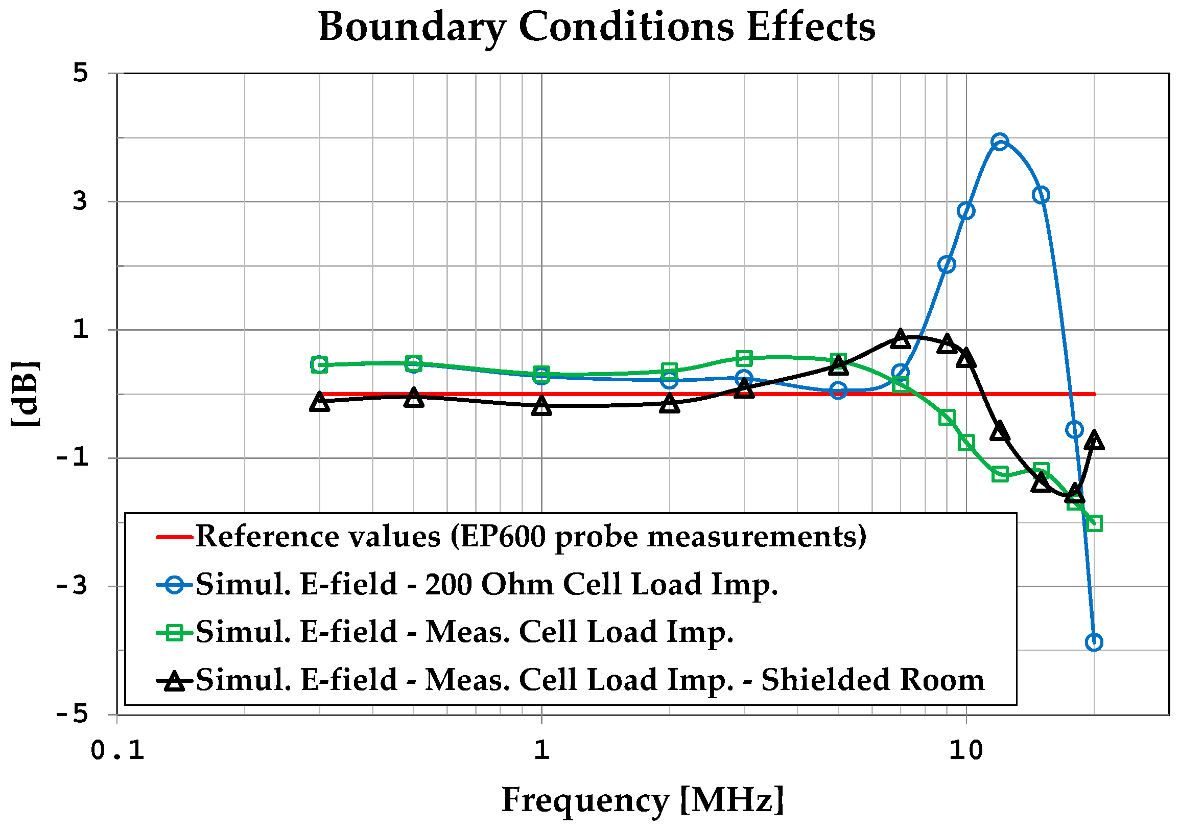
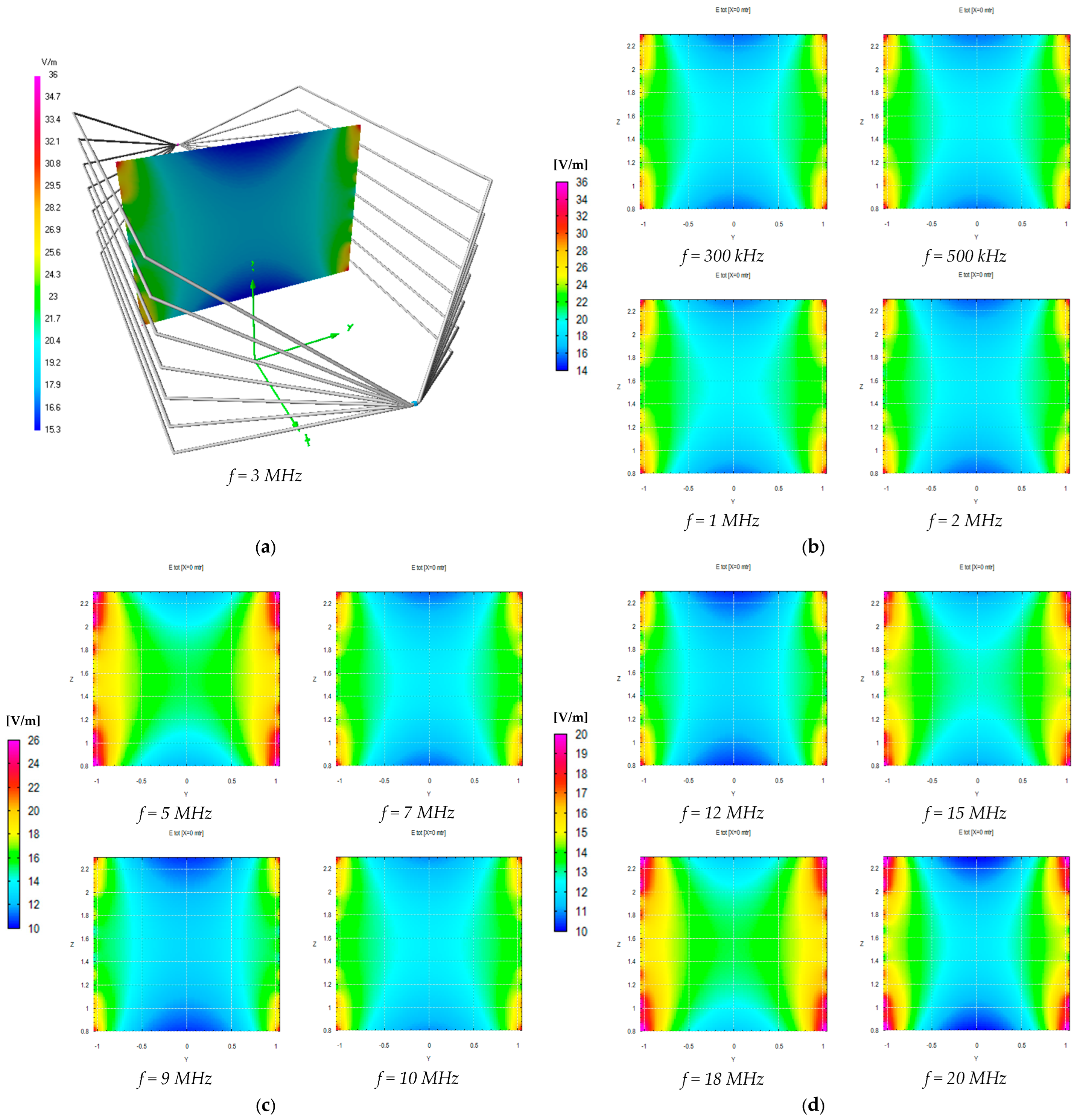
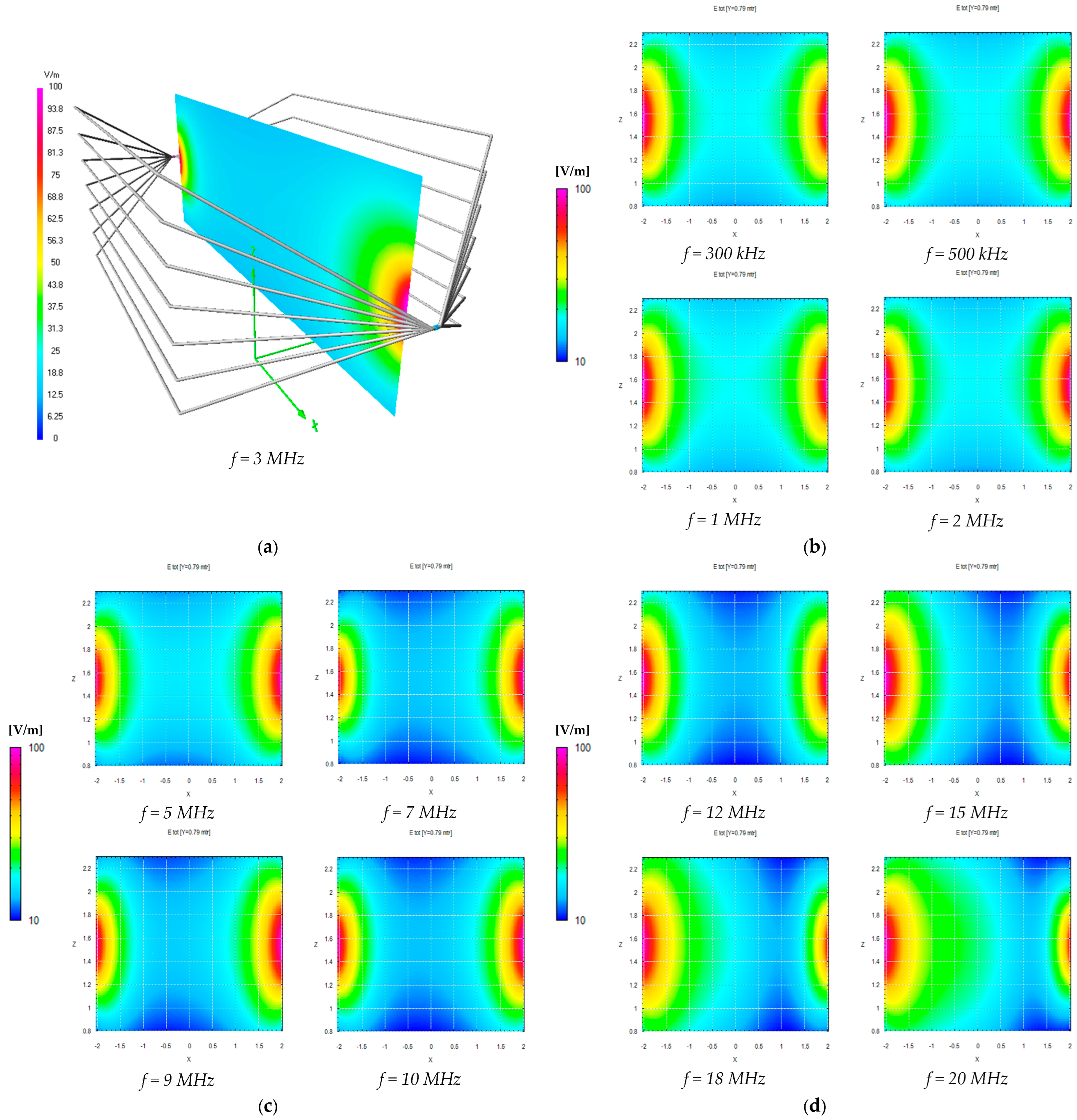
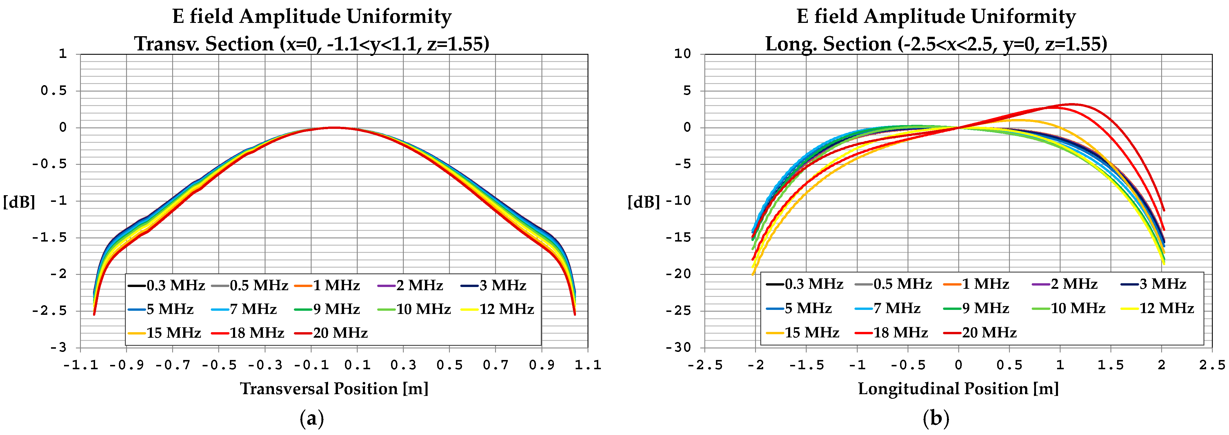
4. Numerical and Experimental Assessment of the Electric Field Generated by the MWTEM Transmission Line

Due to the absence of detailed technical documentation about the spatial distribution of the field generated by the MWTEM transmission line, before its use for area monitor calibration and evaluation, the distribution and uniformity of the electric field generated inside its useful volume was analyzed by means of both numerical simulations and measurements. For simulations, at the input port of the line (between the balun and the tapered section), the same set of applied peak-to-peak voltage amplitudes V_p-p used during the experimental activities was considered. As shown in Figure 4b, the voltages were detected by means of a suitable differential probe connected to the balanced input port of the MWTEM transmission line and with the help of a digital oscilloscope. The numerical simulations were performed with a method of moment (MoM) algorithm by using a model of the MWTEM transmission line developed according to the guidelines of the employed software, i.e., the Numerical Electromagnetics Code (NEC). As described in detail in [29,30,31], NEC uses both an electric field integral equation (EFIE) and a magnetic field integral equation (MFIE) to model the electromagnetic response of systems composed of conductive wires and surfaces. Each formulation has advantages for specific cases: EFIE is well suited for small-volume thin-wire structures, while MFIE works well for large surfaces. Assuming a time-harmonic dependance $e^{j\omega t}$, under the assumption of thin wires, the electric field integral equation (EFIE) can be written as [29,30,31]:

$$-\widehat{n}\left(\overrightarrow{r}\right)\times {\overrightarrow{E}}^I\left(\overrightarrow{r}\right)=-{\displaystyle \frac{j\eta }{4\pi k}}\widehat{n}\left(\overrightarrow{r}\right)\times {\int }_{L}I\left(s^{\prime }\right)\left(k^2{\widehat{s}}^{\prime }-\nabla {\displaystyle \frac{\partial }{\partial s^{\prime }}}\right)g\left(\overrightarrow{r},\overrightarrow{r}\prime \right)ds\prime$$

(1)

where:

$$g\left(\overrightarrow{r},\overrightarrow{r}\prime \right)={\displaystyle \raisebox{1ex}{$e^{-jk\left|\overrightarrow{r}-\overrightarrow{r}\prime \right|}$}\!\left/ \!\raisebox{-1ex}{$\left|\overrightarrow{r}-\overrightarrow{r}\prime \right|$}\right.}$$

${\overrightarrow{E}}^I$ is an incident electric field;

$k=\omega \sqrt{{\mu }_0{\epsilon }_0}$, $\eta =\sqrt{{\mu }_0/{\epsilon }_0}$;

$\overrightarrow{r}$ is the observation point;

$\widehat{n}\left(\overrightarrow{r}\right)$ is the unit normal vector of the surface at $\overrightarrow{r}$;

$I$ is the current flowing in the wire having length L;

$s$ is the distance parameter along a wire axis;

$\widehat{s}$ is the unit vector tangent to wire axis.

The magnetic field integral equation (MFIE) can be written as:

$$-\widehat{n}\left({\overrightarrow{r}}_0\right)\times {\overrightarrow{H}}^I\left({\overrightarrow{r}}_0\right)=-{\displaystyle \frac{1}{2}}{\overrightarrow{J}}_s\left({\overrightarrow{r}}_0\right)+{\displaystyle \frac{1}{4\pi }}{\int }_S\widehat{n}\left({\overrightarrow{r}}_0\right)\times \left[{\overrightarrow{J}}_s\left(\overrightarrow{r}\prime \right)\times \nabla \prime g\left({\overrightarrow{r}}_0,\overrightarrow{r}\prime \right)\right]dA\prime$$

(2)

where:

${\overrightarrow{H}}^I$ is an incident magnetic field;

${\overrightarrow{J}}_S$ is a surface current density induced on a surface S;

${\overrightarrow{r}}_0$ is a surface point;

$\widehat{n}\left({\overrightarrow{r}}_0\right)$ is the unit vector normal to S at ${\overrightarrow{r}}_0$.

The integral Equations (1) and (2) are solved numerically in NEC by the method of moments (MoM) [32]. A brief review of this method is provided in Appendix B.

The ${\overrightarrow{E}}_{tot}$ amplitudes were calculated for a discrete set of frequencies using the NEC implementation available in the 4NEC2 (V. 5.9.3) software package [31], considering a plane transversal to the line axis (x-axis) being placed in the center of the length of line (x = 0 m) and a plane parallel to the line axis (x-axis) and orthogonal to the y-axis (i.e., a longitudinal plane). The geometry of the MWTEM transmission line and the axes of the coordinate system are shown in Figure 3. The main parameters of the simulations and the results obtained in the central position of the transversal and longitudinal sections (x = 0, y = 0, z = 1.55 m) are summarized in

Table 2. MWTEM transmission line—simulation parameters and results.

Freq. [MHz]	Applied Voltage [Vp-p]	EP600 Meas. [V/m]	$\left|{\overrightarrow{\mathit{E}}}_{\mathit{t}\mathit{o}\mathit{t}}\right|$ calc. 1 [V/m]	$\left|{\overrightarrow{\mathit{E}}}_{\mathit{t}\mathit{o}\mathit{t}}\right|$ Simul. (Znom = 200 Ω) [V/m]
0.3	162.5	17.93	24.52	18.86
0.5	162.5	18.02	24.74	19.01
1	164.5	18.57	24.91	19.17
2	158.3	17.95	23.83	18.40
3	153.1	17.48	23.18	17.97
5	133.3	15.75	20.17	15.85
7	113.3	13.30	17.37	13.82
9	139.5	13.42	21.25	16.93
10	145.8	12.75	22.37	17.71
12	160.4	11.81	24.26	18.57
15	176.1	12.99	26.81	18.58
18	150.0	14.62	22.50	13.71
20	114.5	15.31	17.37	9.80

¹ Value calculated with the formula $\left|\overrightarrow{E}\right|={\displaystyle \raisebox{1ex}{$V_{rms}$}\!\left/ \!\raisebox{-1ex}{$d$}\right.}$, where d = 2.32 m.

and

Table 3. MWTEM transmission line—effects of measured load impedance values and of a shielded chamber.

Freq. [MHz]	Zmeas. [Ω]	$\left|{\overrightarrow{\mathit{E}}}_{\mathit{t}\mathit{o}\mathit{t}}\right|$ Simul. [V/m]	$\left|{\overrightarrow{\mathit{E}}}_{\mathit{t}\mathit{o}\mathit{t}}\right|$ Simul. (with Shield) [V/m]
0.3	201-j5	18.86	17.67
0.5	201-j8	19.04	17.93
1	200-j15	19.25	18.20
2	196-j30	18.71	17.63
3	189-j43	18.64	17.67
5	171-j58	16.71	16.59
7	153-j72	13.53	14.70
9	133-j79	12.87	14.74
10	124-j80	11.69	13.62
12	107-j80	10.23	11.07
15	86-j74	11.32	11.10
18	68-j64	12.04	12.25
20	58-j51	12.14	14.11

. In Table 2, for each frequency value considered, the following data are reported: the peak-to-peak voltage values V_p-p applied at the balanced input port of the MWTEM line, the electric field amplitudes measured with an EP600 field probe, the field value calculated with the formula $\left|\overrightarrow{E}\right|={\displaystyle \raisebox{1ex}{$V_{rms}$}\!\left/ \!\raisebox{-1ex}{$d$}\right.}$ (where d = 2.32 m is the distance between the two halves of the MWTEM line in the central section), and the simulated field values obtained assuming a constant 200 Ω load.

For a more accurate characterization of the device, the complex values of the load impedance (composed of non-inductive high-power resistances) were measured with a network analyzer, because, as expected, they differed markedly from the nominal value (200 Ω) because of the non-ideal behavior of the lumped components making up the load. Table 3 reports, for each frequency, the measured complex load impedance values and the simulated electric field amplitudes (obtained with the measured load impedances). To evaluate the effects and take them into account, simulations were also performed with the MWTEM line being placed inside a shielded chamber having the characteristics reported in Table 1 and pictured in Figure 4.

An initial observation from Table 2 is that the formula $\left|\overrightarrow{E}\right|={\displaystyle \raisebox{1ex}{$V_{rms}$}\!\left/ \!\raisebox{-1ex}{$d$}\right.}$ always overestimates the actual field values. In Figure 5, the results obtained with the MoM algorithm are graphed and compared with the measured values. By analyzing the plots in Figure 5, we can observe that the simulations assuming a constant resistive load (200 Ω) provide a good representation of the field amplitude up to about 7 MHz, while for higher frequencies, it is necessary to use the actual load impedance.

We can also observe good accordance between measurements and simulations, in particular between the values measured with the EP600 probe and those obtained by simulations considering the measured load impedances and the effects of the shielded chamber. These results confirm the effectiveness of the model used for the simulations, in particular for the field uniformity analysis. The measurements taken with the EP600 probe can be assumed to be reliable as this device is very small, battery-operated, and connected to a PC with control software through a fiber optic cable, allowing for high measurement accuracy. Taking the field amplitude measured with the EP600 probe as a reference, Figure 6 shows the deviations observed with three different boundary conditions assumed during the simulations: the MWTEM line with the nominal load impedance (200 Ω), MWTEM line with the measured load impedance, and MWTEM line with the measured load impedance inside the shielded chamber. The plots in Figure 6 confirm the important role of the load and indicate that the use of the effective impedance values of the load greatly increases the accuracy of the calculated field values; in addition, the shielded chamber appears to have had an appreciable but limited effect. Excluding the configuration with nominal load impedance, the effects of the boundary conditions are evident for frequencies higher than about 8 MHz, where deviations of about 2 dB can be observed. For lower frequencies, the deviations are very small (about ± 0.5 dB); the limited effect of the shielding chamber confirms that the electric field is mainly confined within the useful volume of the MWTEM line, as occurs in static conditions. To evaluate the uniformity of the electric field generated by the MWTEM line, the results obtained in the two orthogonal planes were analyzed in detail. Figure 7b–d presents the plots of simulated $\left|{\overrightarrow{E}}_{tot}\right|$ values in the transversal plane, while the corresponding plots in the longitudinal plane can be observed in Figure 8b–d. The simulations were performed for the same set of frequency values considered during the experimental activities, listed in Table 2, with a step of 1.5 cm (along x, y and z) for the electric field calculation in both the transversal and the longitudinal planes. As can be observed in Figure 7 and Figure 8, in the central volume of the MWTEM transmission line, the electric field amplitude is sufficiently uniform. In more detail, the plots in Figure 9 show the difference (in dB) between the field amplitude in the central position (x = 0, y = 0, z = 1.55 m) and the values calculated moving along the y-direction (−1.1 < y < 1.1 m, Figure 9a) and along the x-direction (−2.5 < x < 2.5 m, Figure 9b).

By analyzing these data, it can be observed that the field in the central zone shows small and regular variations: about 1.5 dB for a position variation of ±0.9 m in the transversal plane and about 2 dB for a position variation of ±0.5 m in the longitudinal plane. Taking into account that in a TEM structure the electric field is almost transversal, its proper use is to host the area monitor with the axis lying in the transversal plane, where the electric field amplitude is sufficiently uniform in a spatial interval adequate to host the device under testing. The electric field generated for the area monitor calibration is in practice in the near-field region with respect to the field sources; then, to verify the existence in the volume formed by the MWTEM transmission line of a TEM field configuration, a detailed numerical analysis of the field components was also carried out. The analysis was performed on a transversal and a longitudinal cross-section, having the dimensions 1 × 1 m. The results, reported in detail in Appendix C, allowed us to verify that, according to the TEM configuration definition, the longitudinal components of both the electric field vector and the magnetic field vector are negligible if compared with the transversal components. In addition, it was also possible to confirm that the electric field vector is mainly directed along the transversal y-direction and the magnetic field along the transversal z-direction (i.e. the electric and the magnetic fields are mutually orthogonal).

The models of the experimental setup, in free space and inside the shielded chamber, followed the modeling guidelines of the NEC software [31]. The metallic enclosure of the shielded chamber was formed with wire grids according to the modelling concepts given in [33,34,35] for conductive surfaces. The use of the discretization criteria given in [31] (expressed in terms of the length of the segments composing the wires of the MWTEM structure, normalized to the wavelength) guarantees the high accuracy of the results. Some details about the models and the computational effort are summarized in

Table 4. NEC model parameters and simulation effort details.

NEC Model	Number of Segments	Simulation Time 1 [s]
MWTEM in free space	2100	30
MWTEM inside shielded chamber	9062	1743

¹ Simulation time necessary for each frequency value.

. All of the simulations were carried out on a personal computer equipped with an Intel Core i7 CPU 2.10 GHz and with 8 GB of RAM.

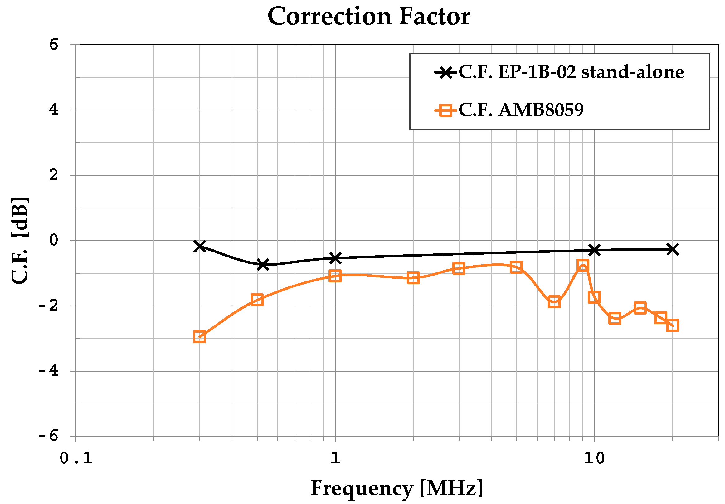
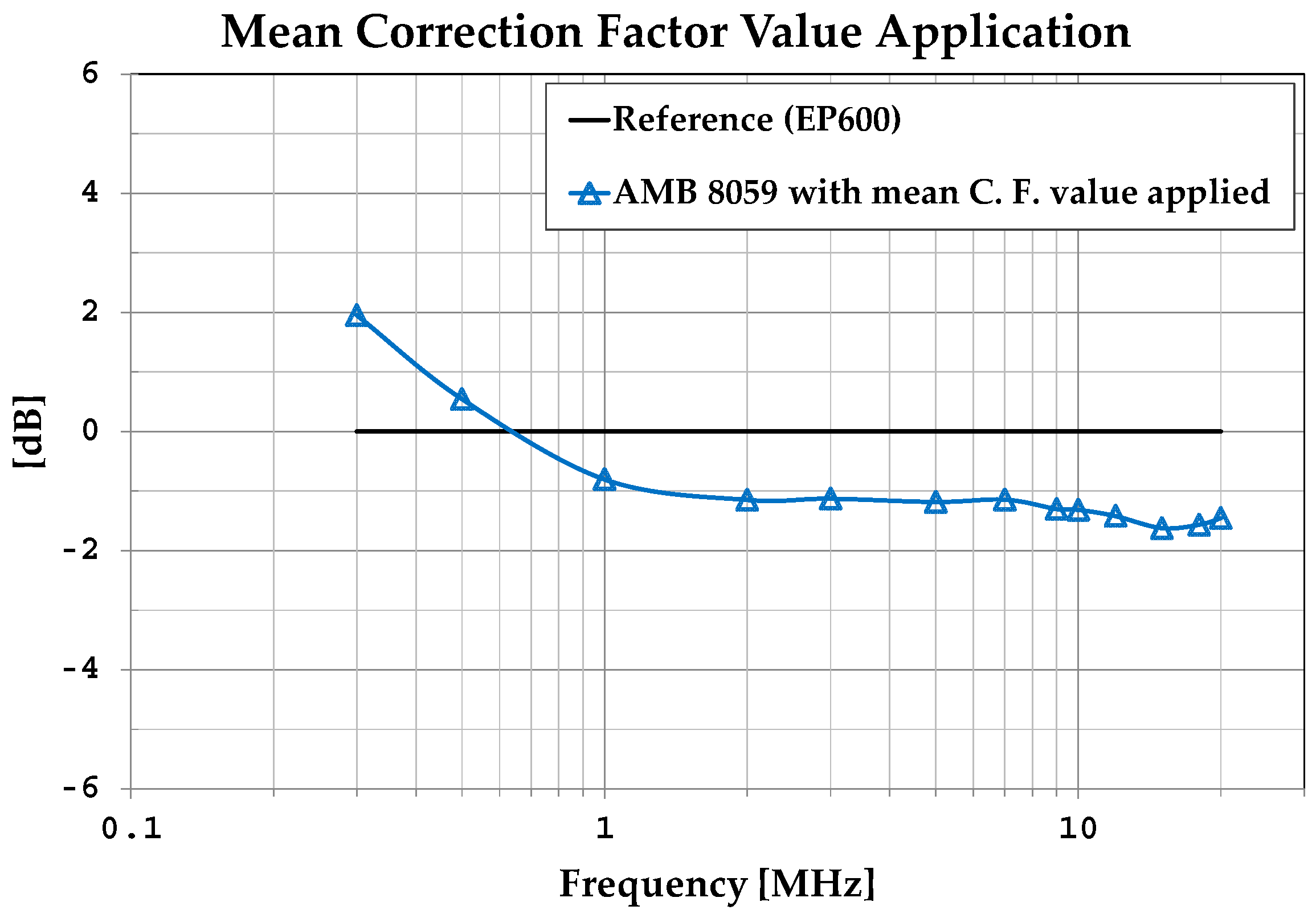
5. Experimental Evaluation and Calibration of the EMF Area Monitor

After completing the assessment of the uniformity of the electric field generated in the central volume of the MWTEM transmission line using an EP600 field probe as a reference, the field generated by the MWTEM line was employed to evaluate and calibrate the AMB-8059 area monitor (provided by NARDA STS S.r.l., Cisano sul Neva, Savona, Italy) equipped with a solar panel and an EP-1B-02 wideband probe (frequency band 0.1–3000 MHz, amplitude range 0.2–200 V/m). This made it possible to evaluate the frequency behavior of the area monitor (equipped with the EP-1B-02 probe as a unique field sensor) and determine its correction factor (C.F.), defined, as in (3), at a given frequency and with a fixed electric field amplitude, as the ratio of the simulated electric field amplitude in the central position of the MWTEM line (assumed as the reference field level $E_{REF.}$) to the measurement ($E_{MEAS.}$) obtained with the area monitor placed with the EP-1B-02 probe in the same position:

$$C.F. \left[dB\right]=20{Log}_{10}\left({\displaystyle \frac{E_{REF.}}{E_{MEAS.}}}\right)$$

(3)

In practice, during real on-site measurement activities, the correction factor has to be applied to the measured field to obtain the effective value of the field under measurement. This is performed manually, or automatically if the C.F. is stored in the area monitor’s control module. In Figure 10, the C.F. obtained for the area monitor as a whole instrument is compared with the correction factor of the EP-1B-02 probe calibrated as a stand-alone device. As expected, the frequency response of the field probe integrated into the area monitor is not the same as that of the probe alone; when integrated within the area monitor, the probe shows a less uniform frequency behavior and also proves to be a bit more sensitive (differences vary between 0.5 dB and 2.7 dB).

Knowing the C.F. makes it possible to improve measurement accuracy when a source with a known spectrum position is under measurement; the availability of a correction factor is of paramount importance in several practical cases where the area monitor is placed in the proximity of a known source deemed to be continuously monitored. When the spectral position of the source is known, the use of the precise C.F.—valid for the emission frequency of the source—allows for the optimum improvement of measurement accuracy, especially if the C.F. is available with a sufficiently small frequency step. In addition, when electromagnetic pollution is generated by unknown sources, the frequency behavior of the correction factor can be used to define a mean value to be applied to measurements in order to reduce uncertainty. Regarding different types of sources, we assume a source to be known if its emission frequency band is identified. For example, a source is considered to be known if it generates an exposure level at a site and is associated with a broadcasting system whose emission frequency is known either from the system owner or from preliminary spectral narrow-band measurements. Conversely, a source is considered unknown at a site where no information on its emission spectrum is available from the owner or from narrow-band measurements. In addition, knowing the emission frequency bands of multiple sources is ineffective if they all contribute to a non-negligible exposure level at the same site. In such cases, it is impossible to apply different C.F.s to measurements taken with wideband probes (such as those integrated into the area monitor) as they provide only a single measurement value, representing the combined effects of all sources. Therefore, when dealing with unknown sources, using a single C.F. value—such as the mean C.F.—is likely the best approach.

To verify the effectiveness of using the mean C.F. value, an electric field was generated in the MWTEM line and measured in its central position with the area monitor at the same frequencies considered for the calibration. The deviations of the measurements taken with the area monitor after the application of the mean C.F. value from the measurements taken under the same conditions with the EP600 probe (assumed as references) are shown in Figure 11. We can observe that the application of a mean constant C.F. for frequencies higher than 1 MHz makes the sensor’s frequency response uniform and implies errors of about 1 dB; for frequencies lower than 1 MHz, it implies higher yet still limited errors of around 2 dB.

Future activities will investigate the feasibility of specific correction factors associated with different ambient area configurations, e.g., those equipped with devices and cables for specific applications. Further analysis will also be performed to evaluate the uncertainty associated with the correction factor measurement procedure.

6. Conclusions

The electric field generated by an MWTEM transmission line was analyzed in detail, both numerically and experimentally, to evaluate its capability to generate for f < 30 MHz a controlled electric field sufficiently uniform for the exposure of the entire structure of an EMF area monitor. Typically, the field probe integrated in an area monitor is calibrated as a stand-alone device without taking into account possible effects on the probe response due to electromagnetic interaction with the area monitor structure and materials. To avoid such problems and improve measurement accuracy, the ambient area monitor was calibrated by exposing the whole structure of the device to the electric field generated by the previously characterized MWTEM line. A frequency-varying correction factor (C.F.) to be applied in the case of known field sources was determined, and the effectiveness of using a mean (constant) C.F. value in the case of unknown sources was evaluated.

References

1. International Commission on Non-Ionizing Radiation Protection. Guidelines for limiting exposure to time-varying electric and magnetic fields (1Hz–100 kHz). Health Phys. 2010, 99, 818–836. [Google Scholar] [CrossRef] [PubMed]
2. International Commission on Non-Ionizing Radiation Protection. Guidelines for limiting exposure to electromagnetic fields (100 kHz to 300 GHz). Health Phys. 2020, 118, 483–524. [Google Scholar] [CrossRef] [PubMed]
3. European Union. Directive 2013/35/EU on the Minimum Health and Safety Requirements Regarding the Exposure of Workers to the Risks Arising from Physical Agents (Electromagnetic Fields) and Repealing Directive 2004/40/EC; Council of the European Union: Brussels, Belgium, 2013. [Google Scholar]
4. European Union (UE) Council Recommendation. Council Recommendation of 12 July 1999 on the Limitation of Exposure of the General Public to Electromagnetic Fields (0 Hz to 300 GHz)—(1999/519/EC); Council of the European Union: Brussels, Belgium, 1999. [Google Scholar]
5. International Telecommunication Union (ITU). Recommendation ITU-T K.83—Monitoring Electromagnetic Field; International Telecommunication Union (ITU): Geneva, Switzerland, 2011. [Google Scholar]
6. Ioriatti, L.; Martinelli, M.; Viani, F.; Benedetti, M.; Massa, A. Real-time distributed monitoring of electromagnetic pollution in urban environments. In Proceedings of the IEEE Geoscience and Remote Sensing Symposium (IGARSS 2009), Cape Town, South Africa, 12–17 July 2009. [Google Scholar]
7. Viani, F.; Donelli, M.; Oliveri, G.; Massa, A.; Trinchero, D. A WSN-based system for real-time electromagnetic monitoring. In Proceedings of the IEEE International Symposium on Antennas and Propagation (APSURSI), Spokane, DC, USA, 3–8 July 2011. [Google Scholar]
8. Viani, F.; Polo, A.; Donelli, M.; Giarola, E. A Relocable and Resilient Distributed Measurement System for Electromagnetic Exposure Assessment. IEEE Sens. J. 2016, 16, 4595–4604. [Google Scholar] [CrossRef]
9. Antic, D.; Djuric, N.; Kljajic, D. Environmental EMF monitoring in the SEMONT system using quad-band AMB 8057/03 sensor. In Proceedings of the IEEE 10th International Conference on Wireless and Mobile Computing, Networking and Communications (WiMob), Larnaca, Cyprus, 8–10 October 2014. [Google Scholar]
10. Antic, D.; Djuric, N.; Kljajic, D. The AMB 8057-03 sensor node implementation in the SEMONT EMF monitoring system. In Proceedings of the IEEE 12th International Symposium on Intelligent Systems and Informatics (SISY), Subotica, Serbia, 11–13 September 2014. [Google Scholar]
11. Kundacina, O.; Vincan, V.; Antic, D.; Kljajic, D.; Kasas-Lazetic, K. The AMB 8057 utilization for SEMONT’s EMF monitoring in a closed room. In Proceedings of the 24th Telecommunications Forum (TELFOR), Belgrade, Serbia, 22–23 November 2016. [Google Scholar]
12. Djuric, N.; Kavecan, N.; Kljajic, D.; Mijatovic, G.; Djuric, S. Data Acquisition in Narda’s Wireless Stations based EMF RATEL Monitoring Network. In Proceedings of the 2019 International Conference on Sensing and Instrumentation in IoT Era (ISSI), Lisbon, Portugal, 29–30 August 2019. [Google Scholar]
13. Djuric, N.; Kavecan, N.; Radosavljevic, N.; Djuric, S. The Wideband Approach of 5G EMF Monitoring. In Proceedings of the 12th EAI International Conference (AFRICOMM 2020), Ebène City, Mauritius, 2–4 December 2020. [Google Scholar]
14. Jadhav, A.V.; Patil, A.P.; Ajwilkar, P.G.; Nadkarni, R.N.; Bhise, S. Continuous RF monitoring. In Proceedings of the 2nd International Conference on Applied and Theoretical Computing and Communication Technology (iCATccT), Bangalore, India, 21–23 July 2016. [Google Scholar]
15. Carciofi, C.; Garzia, A.; Valbonesi, S.; Gandolfo, A.; Franchelli, R. RF electromagnetic field levels extensive geographical monitoring in 5G scenarios: Dynamic and standard measurements comparison. In Proceedings of the 2020 International Conference on Technology and Entrepreneurship (ICTE), Bologna, Italy, 21–23 September 2020. [Google Scholar]
16. Wang, S.; Chikha, W.B.; Zhang, Y.; Liu, J.; Conil, E.; Jawad, O.; Ourak, L.; Wiart, J. RF Electromagnetic Fields Exposure Monitoring using Drive Test and Sensors in a French City. In Proceedings of the XXXVth General Assembly and Scientific Symposium of the International Union of Radio Science (URSI GASS), Sapporo, Japan, 19–26 August 2023. [Google Scholar]
17. Lee, A.K.; Jeon, S.; Wang, S.; Wiart, J.; Choi, H.D.; Moon, J.I. Population Density and DL EMF Exposure Levels by Region in Korea. In Proceedings of the 2024 IEEE Asia-Pacific Microwave Conference (APMC), Bali, Indonesia, 17–20 November 2024. [Google Scholar]
18. Liu, S.; Tobita, K.; Onishi, T.; Taki, M.; Watanabe, S. Electromagnetic field exposure monitoring of commercial 28-GHz band 5G base stations in Tokyo. Bioelectromagnetics 2024, 45, 281–292. [Google Scholar] [CrossRef] [PubMed]
19. Dikmen, I.C. Continuous Monitoring and Modeling of High-Frequency EM Pollution Using Cutting-Edge Regression Techniques. IEEE Access 2025, 13, 46627–46637. [Google Scholar] [CrossRef]
20. Kiouvrekis, Y.; Psomadakis, I.; Vavouranakis, K.; Zikas, S.; Katis, I.; Tsilikas, I.; Panagiotakopoulos, T.; Filippopoulos, I. Explainable Machine Learning-Based Electric Field Strength Mapping for Urban Environmental Monitoring: A Case Study in Paris Integrating Geographical Features and Explainable AI. Electronics 2025, 14, 254. [Google Scholar] [CrossRef]
21. Azaro, R.; Franchelli, R.; Gandolfo, A. Networks of EMF Area Monitor for Distributed Human Exposure Monitoring: Assessment of Performances in Simulated Realistic Scenarios. In Proceedings of the IEEE International Symposium on Measurements & Networking (M&N), Padua, Italy, 18–20 July 2022. [Google Scholar]
22. Azaro, R.; Gandolfo, A. On the Electric Field Distribution in Radiated Emission Rod Antenna Test Setups: Numerical Analysis and Experimental Validation. IEEE Trans. Electromagn. Compat. 2020, 62, 1611–1618. [Google Scholar] [CrossRef]
23. Crawford, M.L. Generation of Standard EM Fields Using TEM Transmission Cells. IEEE Trans. Electromagn. Compat. 1974, 16, 189–195. [Google Scholar] [CrossRef]
24. Groh, C.; Karst, J.P.; Koch, M.; Garbe, H. TEM waveguides for EMC measurements. IEEE Trans. Electromagn. Compat. 1999, 41, 440–445. [Google Scholar] [CrossRef]
25. Karst, J.P.; Groh, C.; Garbe, H. Calculable field generation using TEM cells applied to the calibration of a novel E-field probe. IEEE Trans. Electromagn. Compat. 2002, 44, 59–71. [Google Scholar] [CrossRef]
26. Macnamara, T.M. Handbook of Antennas for EMC, 2nd ed.; Artech House: Norwood, MA, USA, 2018; pp. 273–334. [Google Scholar]
27. Caorsi, S.; Azaro, R. Field Uniformity Measurements in a TEM Cell using the Modulated Scattering Technique. In Proceedings of the International Symposium on Electromagnetic Compatibility EMC 98 ROMA, Rome, Italy, 14–18 September 1998. [Google Scholar]
28. Carbonini, L. Comparison of analysis of a WTEM cell with standard TEM cells for generating EM fields. IEEE Trans. Electromagn. Compat. 1993, 35, 255–263. [Google Scholar] [CrossRef]
29. Burke, G.J.; Poggio, A.J. Numerical Electromagnetics Code—Method of Moments. Available online: https://apps.dtic.mil/sti/tr/pdf/ADA956129.pdf (accessed on 18 January 2025).
30. Poggio, A.J.; Miller, E.K. Integral Equation Solutions of Three-Dimensional Scattering Problems. In Computer Techniques for Electromagnetics; Mittra, R., Ed.; Pergamon Press: New York, NY, USA, 2007; pp. 159–264. [Google Scholar]
31. NEC Based Antenna Modeler and Optimizer. Available online: https://www.qsl.net/4nec2/ (accessed on 18 January 2025).
32. Harrington, R.F. Field Computation by Moment Methods; MacMillan: New York, NY, USA, 1968. [Google Scholar]
33. Ludwig, A. Wire grid modeling of surfaces. IEEE Trans. Antennas Propagat. 1987, 35, 1045–1048. [Google Scholar] [CrossRef]
34. Rubinstein, A.; Rachidi, F.; Rubinstein, M. On wire-grid representation of solid metallic surfaces. IEEE Trans. Electromagn. Compat. 2005, 47, 192–195. [Google Scholar] [CrossRef]
35. Rubinstein, A.; Rostamzadeh, C.; Rubinstein, M.; Rachidi, F. On the use of the equal area rule for the wire-grid representation of metallic surfaces. In Proceedings of the 7th International Zurich Symposium on Electromagnetic Compatibility, Singapore, 28 February–3 March 2006. [Google Scholar]
36. Ramo, S.; Whinnery, J.R.; Van Duzer, T. Fields and Waves in Communication Electronics; Wiley: New York, NY, USA, 1994. [Google Scholar]
37. Haus, H.A.; Melcher, J.R. Electromagnetic Fields and Energy; Prentice-Hall: Englewood Cliffs, NJ, USA, 1989. [Google Scholar]
38. Higgins, D.F. A Method of Calculating Impedance and Field Distribution of a Multi-Wire Parallel Plate Transmission Line Above a Perfectly Conducting Ground. Air Force Weapons Laboratory, Sensor and Simulation Notes, Note 150, February 1972. Available online: https://summa.unm.edu/notes/SSN/note150.pdf (accessed on 10 April 2025).
39. Baum, C.E.; Higgins, D.; Cummings, D.B.; Faulkner, J.E.; Heinberg, M.; Moore, P.; Nelson, E.B.; Price, M.L.; Crewson, W.F.; Naff, J.T. Electromagnetic Design Calculation for ATLAS I, Design 1. Air Force Weapons Laboratory, Sensor and Simulation Notes, Note 153, June 1972. Available online: https://summa.unm.edu/notes/SSN/note153.pdf (accessed on 10 April 2025).
40. Neureuther, A.R.; Fuller, B.D.; Hakke, G.D.; Hohmann, G. A Comparison of Numerical Methods for Thin Wire Antennas. In Proceedings of the URSI Meeting, Boston, MA, USA, 10–12 September 1968. [Google Scholar]
41. Miller, E.K.; Bevensee, R.M.; Poggio, A.J.; Adams, R.; Deadrick, F.J.; Landt, J.A. An Evaluation of Computer Programs Using Integral Equation for the Electromagnetics Analysis of Thin Wire Structures. Lawrence Livermore Laboratory, Interaction Notes, Note 177, March 1974. Available online: http://ece-research.unm.edu/summa/notes/In/0177.pdf (accessed on 25 February 2025).
42. IEC 61000-4-20:2022-11; Electromagnetic Compatibility (EMC)—Part 4–20: Testing and Measurement Techniques—Emission and Immunity Testing in Transverse Electromagnetic (TEM) Waveguides. IEC: Geneva, Switzerland, 2022.
Figure 1. An example of a battery-operated EMF area monitor in a real application scenario (courtesy of NARDA Safety Test Solutions S.r.l.).
Sensors 25 02920 g001
Figure 2. The structure and the main components of an EMF area monitor.
Sensors 25 02920 g002
Figure 3. The geometry of the multi-wire TEM (MWTEM) transmission line.
Sensors 25 02920 g003
Figure 4. Experimental assessment of the electric field distribution generated by the MWTEM transmission line: (a) the line inside a shielded room; (b) measurement of the voltage amplitudes at the balanced input port; (c) electric field amplitude measurements with the EP600 probe in the central position of the line.
Sensors 25 02920 g004
Figure 5. Simulated and measured E-field amplitude in the central position of the MWTEM transmission line.
Sensors 25 02920 g005
Figure 6. Effects of boundary conditions: MWTEM line load value (nominal 200 Ω, measured) and interaction with the shielded chamber.
Sensors 25 02920 g006
Figure 7. Numerical evaluation of the uniformity of the electric field generated inside the volume formed by the MWTEM transmission line: (a) geometry of the line and the transversal section considered for the simulations (results shown for f = 3 MHz); (b) results for f = 0.3 MHz, f = 0.5 MHz, f = 1 MHz, and f = 2 MHz; (c) results for f = 5 MHz, f = 7 MHz, f = 9 MHz, and f = 10 MHz; (d) results for f = 12 MHz, f = 15 MHz, f = 18 MHz, and f = 20 MHz.
Sensors 25 02920 g007
Figure 8. Numerical evaluation of the uniformity of the electric field generated inside the volume formed by the MWTEM transmission line: (a) geometry of the line and the longitudinal section considered for the simulations (results shown for f = 3 MHz); (b) results for f = 0.3 MHz, f = 0.5 MHz, f = 1 MHz, and f = 2 MHz; (c) results for f = 5 MHz, f = 7 MHz, f = 9 MHz, and f = 10 MHz; (d) results for f = 12 MHz, f = 15 MHz, f = 18 MHz, and f = 20 MHz.
Sensors 25 02920 g008
Figure 9. Numerical evaluation of the uniformity of the electric field generated inside the volume formed by the MWTEM transmission line: (a) field behavior along the transversal direction (x = 0, −1.1 < y < 1.1, z = 1.55 m); (b) field behavior along the longitudinal direction (−2.5 < x < 2.5, y = 0, z = 1.55 m).
Sensors 25 02920 g009
Figure 10. Comparison between the C.F. of the EP-1B-02 probe integrated into the area monitor and the C.F. of the EP-1B-02 probe as a stand-alone device.
Sensors 25 02920 g010
Figure 11. Effect of applying the mean C.F. value.
Sensors 25 02920 g011