In this section, we establish a cooperative localization model integrating UAV mobility patterns and estimation-theoretic analysis. The proposed system model consists of four fundamental components: (1) a dynamic UAV network-based localization architecture with cluster-based coordination mechanisms, (2) mobility-aware and communication-efficient quality metrics for cluster formation, (3) CRLB analysis incorporating both measurement uncertainties and motion-induced errors, and (4) an optimization formulation for cluster assignment of UAVs.
3.1. System Architecture and Basic Definitions
In this work, we investigate the cooperative localization problem of M NCTs with a UAV network consisting of N UAVs distributed in 3D space, where ensures system observability. The UAVs are represented by the set , while the NCTs are denoted by set . The position of UAV and NCT is represented by 3D vectors and , respectively. Besides, denotes the velocity of .
To enhance localization accuracy, we adopt a cluster-based architecture where the UAVs are partitioned into
K distinct clusters
collaboratively estimating the position of a designated NCT
with each cluster
. The cardinality of each cluster, denoted by
, represents the number of UAVs in
.
Figure 1 illustrates an example scenario of dynamic UAV clusters for multi-target localization. UAVs in the same cluster are expected to localize the same NCT while communicating with each other.
Let
to denote whether UAV
is clustered into
, where
Then, let set
denote the index set of UAVs in cluster
, i.e.,
.
Besides, let
denote whether cluster
is assigned to localize NCT
, where
3.2. Mobility-Aware Cluster Quality Metrics
Considering the mobility of UAVs and their changing positions, it is essential to maintain cluster nodes within an effective communication range and ensure similar movement trends. This contributes to network topology stability. Moreover, reducing communication overhead and delay within sensing clusters is crucial for preventing frequent topology changes. To achieve these objectives, we introduce three metrics to assess the cooperation quality of UAV clusters: position similarity, velocity similarity, and communication link consistency.
3.2.1. Position Similarity and Velocity Similarity
For any two UAVs, their distance
is measured by the Euclidean distance between their positions
Next, we define the position similarity as follows.
Definition 1 (Position Similarity of a UAV Pair).
Position similarity of and is defined aswhere is a scale factor constant.Besides, we introduce the velocity similarity to evaluate the movement consistency of UAVs within a cluster.
Definition 2 (Velocity Similarity of a UAV Pair).
Velocity similarity of and is defined as cosine similarity
It can be observed that
and
are both symmetric, i.e.,
and
.
Next, we consider the metrics for clusters. To begin with, let
denote the set of 2-element
unordered pairs selected from the index set
of
, as defined by Equation (
6).
To ensure the validity of the subsequent cluster metrics, we restrict our analysis to clusters with
.
The cluster diameter is introduced to evaluate the spatial distribution of UAVs within a cluster.
Definition 3 (Cluster Diameter).
Cluster diameter is defined as the maximum distance between any UAV pairs within the cluster
Definition 4 (Position Similarity of a Cluster).
Position similarity of a cluster is the average position similarity of all UAV pairs within the cluster
Remark 1. When choosing in Equation (4) to compute the position similarity of a UAV pair in the cluster, it is recommended to set to ensure it is within the normalized range . Similarly, the velocity similarity of a cluster can be defined as follows.
Definition 5 (Velocity Similarity of a Cluster).
Velocity similarity of a cluster is the average velocity similarity of all UAV pairs within the cluster
Finally, we define the motion similarity of cluster
Definition 6 (Motion Similarity of a Cluster).
Motion similarity of cluster is defined as the weighted sum of position similarity and velocity similaritywhere is a weight factor. 3.2.2. Communication Link Consistency
The communication link consistency [
22] serves as a critical metric for evaluating information propagation performance in sensor networks. To ensure robust, rapid, and efficient intra-cluster communication among UAVs, we introduce a mobility-based model for communication link consistency.
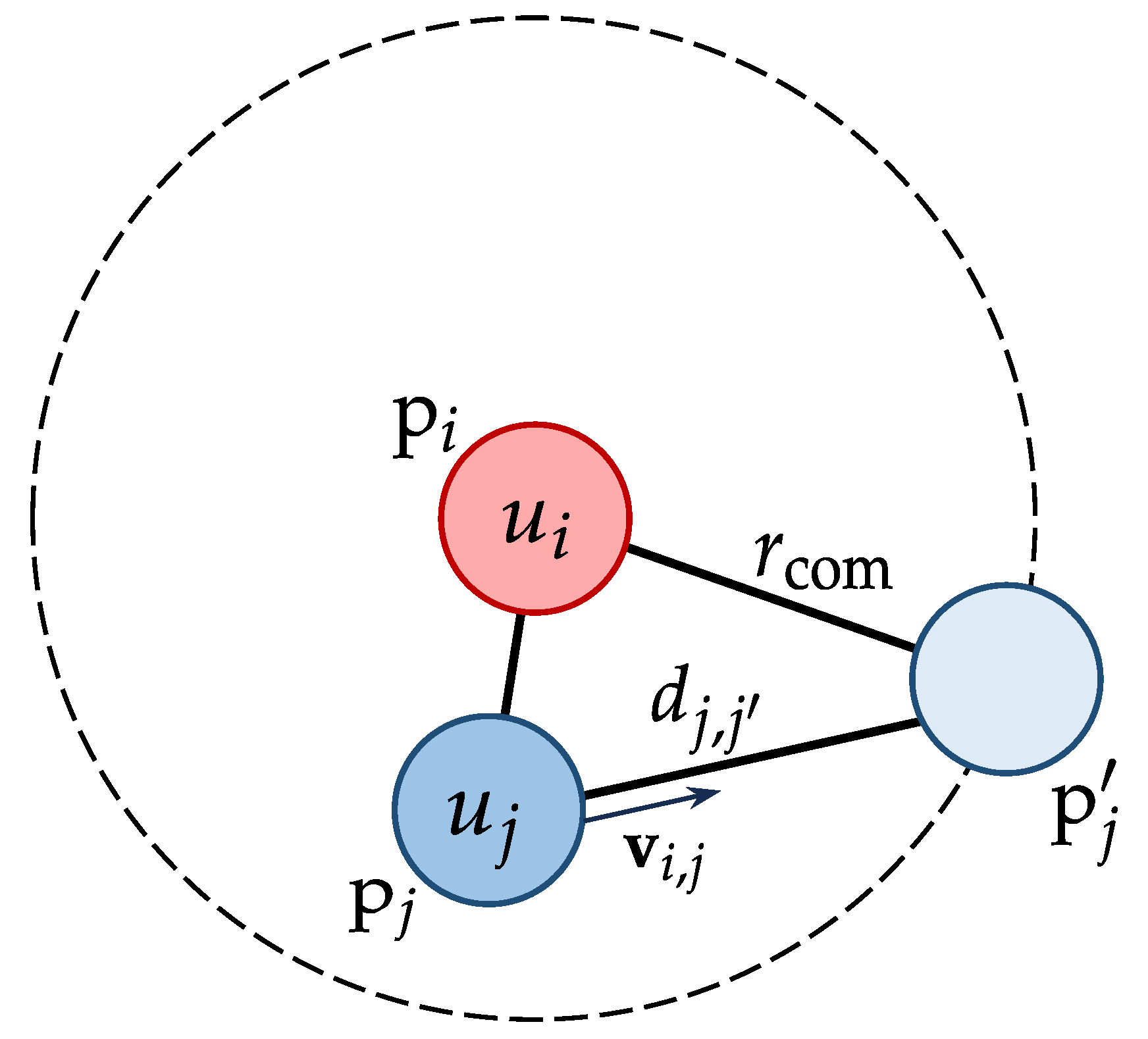
For two mobile UAVs
and
with identical communication radius
, assuming constant relative velocity and direction over a short future time interval, the communication link consistency
is defined as
where
is the relative velocity,
is the projected position of
relative to
when the distance between them exactly reaches
,
is the Euclidean distance between
and the projected position, and
is a time threshold for link stability, as illustrated in
Figure 2.
Next, we define the communication link consistency of a cluster.
Definition 7 (Communication Link Consistency of a Cluster).
Communication link consistency of cluster is the average communication link consistency of all UAV pairs within the cluster 3.3. Cramér–Rao Lower Bound Derivation
The CRLB [
5] is a fundamental benchmark in estimation theory, establishing a theoretical lower bound on the variance in any unbiased estimator. In the context of clustered UAV-based localization, the CRLB provides critical insights into the achievable localization accuracy under specific cluster configurations and measurement models. This section derives the CRLB for the proposed clustered localization framework, explicitly incorporating key factors such as the geometric distribution and velocity of UAVs within clusters, and the statistical properties of measurement errors.
The CRLB derivation builds upon the following fundamental assumptions.
(A1) Measurement independence: Observations from different UAVs are statistically independent, i.e., is independent of for .
(A2) Error normality: Both position errors and motion-induced errors follow zero-mean Gaussian distributions.
(A3) Spatial-temporal uncorrelation: Measurement errors across different time instants and spatial positions are mutually uncorrelated.
Using the TOA model [
23], the real distance between a UAV located at
and an NCT at
is given by
However, real-world observations from UAV
for NCT
are subject to normally distributed errors in sensor time-delay measurements, leading to noisy distance estimates
where
e represents measurement noise. According to [
24], the position error from distance measurement of NCTs follows a zero-mean normal distribution with variance, that is
where
is a proportionality constant.
To transform this error into Euclidean coordinates, the estimated position
of
observed by UAV
n is given by
where
represents the equivalent localization noise, which follows a multivariate normal distribution
where the covariance matrix
can be computed as
where
is the unit vector pointing from the UAV’s position
to the NCT’s
.
Beyond position noise, UAV mobility introduces an additional source of error. The velocity
of UAV
n affects its self-localization accuracy, as positioning measurements from external sensors (e.g., GPS or infrared systems) experience time-delay errors. Assuming the UAV self-localizes at a fixed clock frequency, the positioning error tends to increase with its velocity magnitude
. This inherent localization uncertainty propagates to the position estimation of NCTs, particularly in high-speed scenarios. Consequently, the motion-induced localization error
in Euclidean coordinates follows a multivariate normal distribution
where
is a velocity-dependent covariance matrix computed as
where
is the unit velocity vector, and
is a proportionality constant.
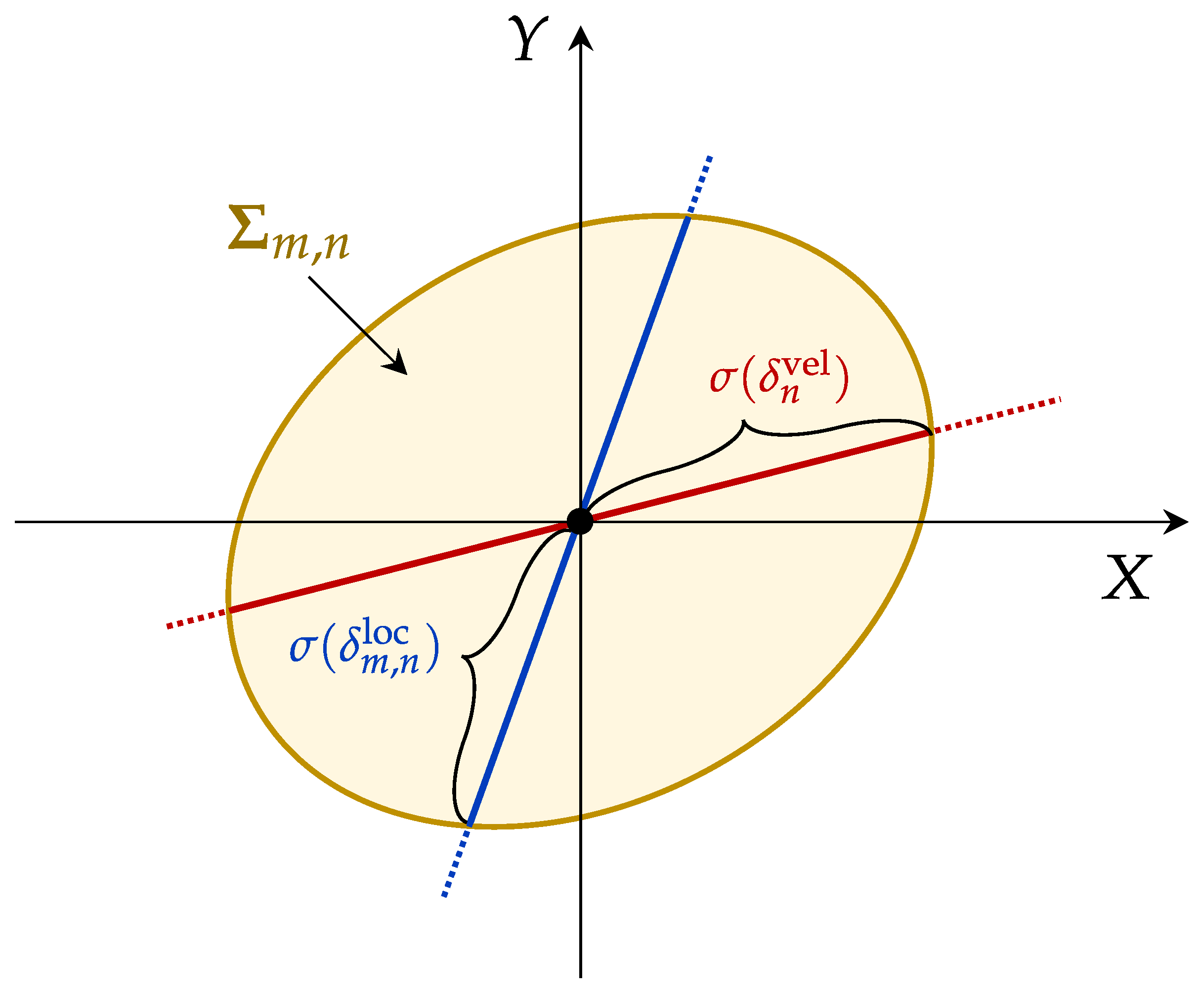
Combining these two sources of error, the total observed localization error for NCT
m as measured by UAV
is
which, according to assumption (A2), follows a multivariate normal distribution,
where the total covariance matrix is given by
Figure 3 illustrates the spatial characteristics and superposition effects of these error components. Note that the resulting composite covariance matrix
may also be singular or ill-conditioned. To address this, we replace the standard matrix inverse with the Moore–Penrose pseudoinverse, denoted as
, ensuring that the inversion required for subsequent calculations (e.g., in the FIM and CRLB computations) remains well-defined.
Following conventional estimation theory [
23,
25,
26], we then employ the CRLB to quantify localization precision. The FIM, denoted as
, serves as the fundamental construct for CRLB computation. For a single observation
, the conditional probability density function (CPDF) is formulated as
The corresponding log-likelihood function becomes
For a UAV cluster
with the UAV index set
assigned to localize NCT
, the joint CPDF under Assumptions (A1) and (A3) is
Then, the aggregate log-likelihood function consequently follows
In 3D Euclidean space, the FIM adopts the symmetric structure
where each element is computed by
where
. Leveraging multivariate normal distribution properties, the FIM simplifies to
The additive structure of FIM
directly results from the assumption (A1), as cross-correlation terms between different UAV observations vanish.
Then, the CRLB
of NCT
m for the configured cluster
is thereby computed as
where
denotes matrix trace and
is the Moore–Penrose pseudoinverse of
.
3.4. Problem Formulation for Optimal Cluster Assignment
We first consider the constraints among UAVs, clusters, and targets. Recall that
x and
y are indicator variables defined by Equations (
1) and (
2). Here, we assume each UAV can only be assigned to one cluster (The framework can be generalized by allowing each UAV to participate in multiple clusters, defined by
, where
specifies the maximum number of clusters UAV
can belong to. This extension maintains mathematical consistency with our model. For simplicity, we focus on the case that
in this paper.), i.e.,
, while each cluster corresponds to one NCT, i.e.,
and
,
. Besides, each cluster must have at least
c UAVs, i.e.,
, which also implies that the total number of UAVs must be at least
c times the number of NCTs. Additionally, each cluster has a maximum radius constraint, i.e.,
.
Next, we define the objective function. For an NCT
, both motion similarity
and communication link consistency
of its corresponding cluster
should be maximized to ensure effective collaboration while its CRLM
should be minimized to ensure localization performance. Thus, the objective function considering all NCTs and their corresponding clusters is formulated as
where
indicates that
k is the index of the cluster assigned to the NCT
decided by
y, and
are weight factors.
Thus, the optimization problem is formulated as P1.
The formulated optimization problem is a zero-one programming problem, where the decision variables
x and
y are binary integers indicating the assignment of UAVs to clusters and the corresponding relationship between NCTs and clusters.
The formulated optimization problem P1 is computationally challenging due to multiple interrelated factors. First, the objective function involves nonlinear matrix operations through the CRLB term . These operations include nested matrix inversions and trace computations, leading to a non-convex structure with many local minima. Second, the discrete constraints (C1)–(C4) introduce an NP-hard combinatorial structure.
While the original formulation P1 captures the full complexity of dynamic UAV clustering, its direct solution remains computationally intractable due to high-dimensional combinatorial search. Given the constraints (C2) and (C3) in the optimization problem P1, the variable
y constitutes a permutation matrix, which inherently implies that the equality
must hold. This relationship leads to two significant consequences: First,
becomes a single-valued function, allowing to use
to represent
for simplicity. Second, the correspondence between
m and
k establishes a bijective mapping. Consequently, each cluster
can be uniquely associated with a certain NCT
, enabling direct parameterization through either cluster indices
or NCT indices
. In this paper, we adopt the cluster index notation. Thus, the reformulated problem becomes P2.
The reformulated P2 is also a zero-one programming problem, where the decision variables x are binary integers. Even after simplification, P2 retains its non-convex and non-linear nature, making it challenging to solve. Therefore, it is necessary to establish an efficient algorithm to find a solution within a reasonable amount of computational time.


