
Cross-Domain Fault Diagnosis of Rotating Machinery Under Time-Varying Rotational Speed and Asymmetric Domain Label Condition


Abstract
1. Introduction
- (1)
- We construct the model’s input features with physical priors through angular resampling, which explicitly reduces the distribution drift of the signal on the time scale. This makes the IFD model interpretable during the process of learning the discriminative features independent of the rotational speed in the condition-monitoring data;
- (2)
- We propose a label-positioning information compensation mechanism for the discriminative learning of shared and unknown classes in the source and target domains by sample-wise alignment learning and class-wise alignment learning. ASY-WLB uses a prediction margin index (PMI) to determine the probability that samples belong to shared classes, thereby increasing confidence in the correspondence between the samples from the target domain and pseudo-labels from the classifier outputs;
- (3)
- We used balanced learning of intra-class compactness and inter-class separation. To effectively leverage the known sample-type versus the private sample-type potential label information, we proposed a weighted contrastive domain discrepancy (WCDD) loss that aims to minimize the distance between similar samples and maximize the distance between dissimilar samples implicitly, and embed this into the learning process of the ASY-WLB models.
2. Methodology
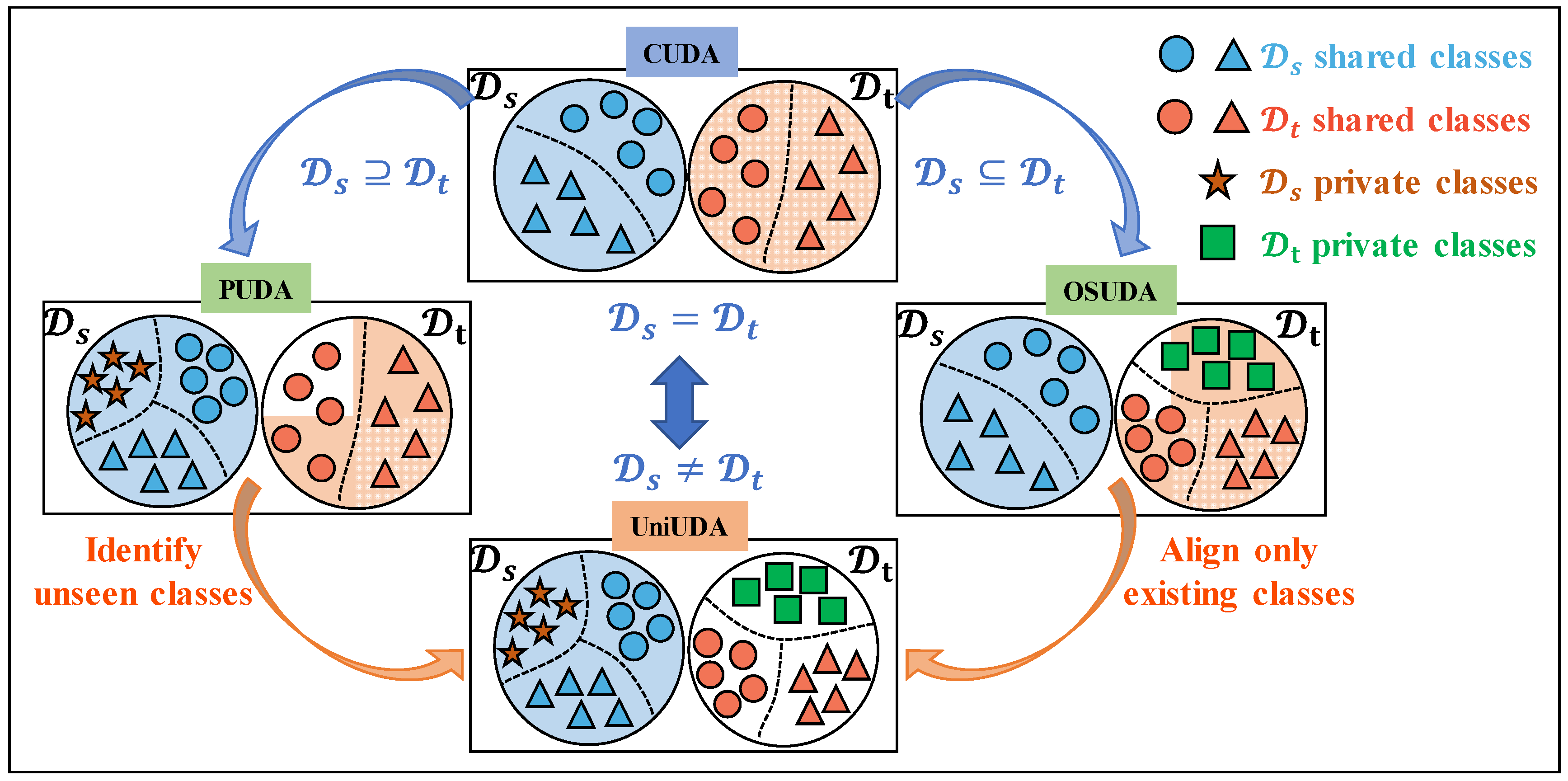
2.1. Problem Formulation
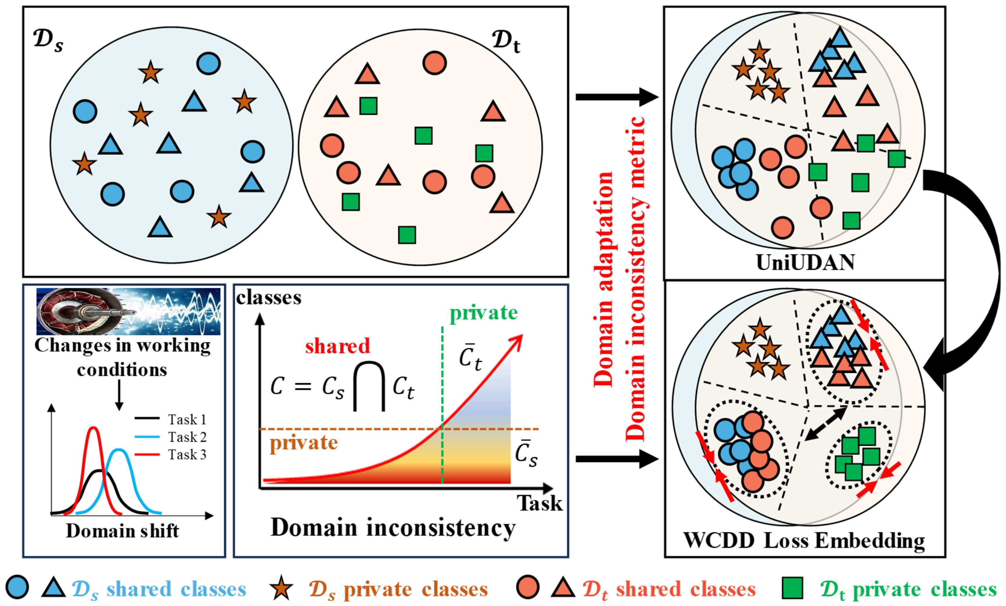
2.2. Representation of Rotational Speed-Independent Transferable Features
2.3. Cross-Domain IFD Method Based on ASY-WLB
2.3.1. IFD Method Across Asymmetric Domain Based on UniUDAN
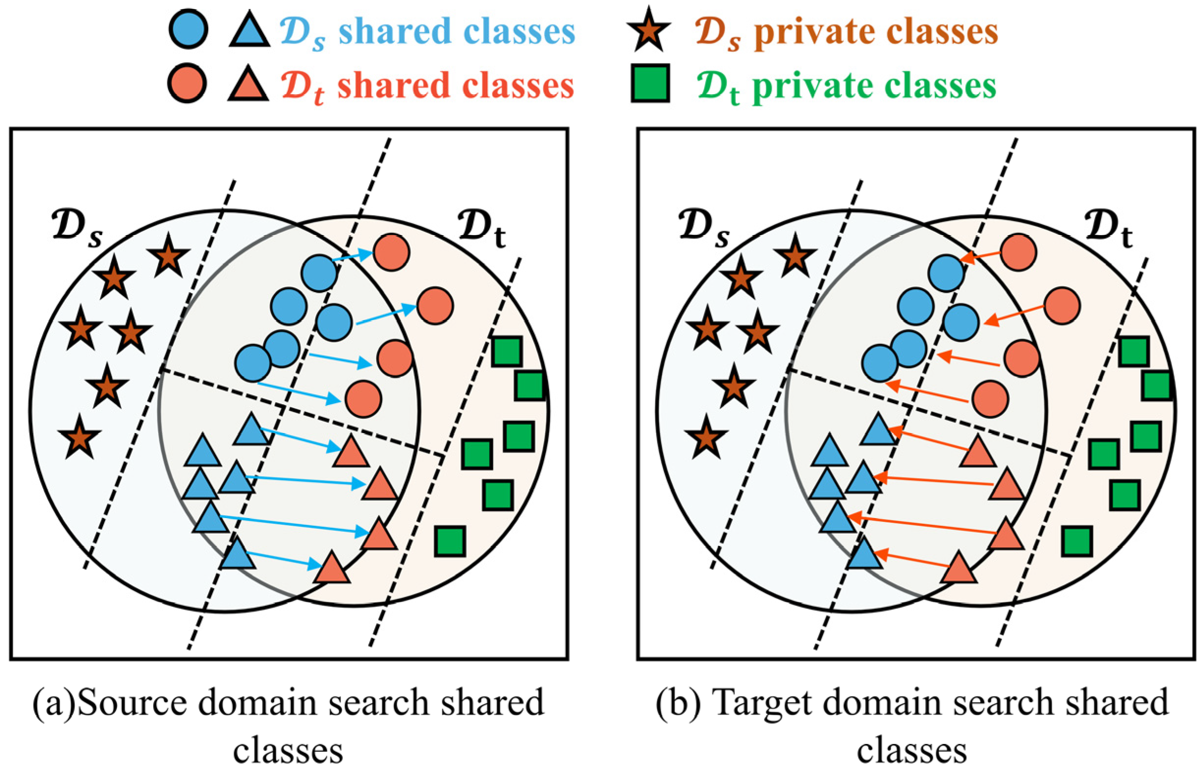
2.3.2. Label-Positioning Information Compensation Mechanism
2.3.3. Balanced Learning of Intra-Class Compactness and Inter-Class Separation
- (1)
- First, ASY-WLB utilizes and to output the conditional distribution (denoted as ) in and the conditional distribution (denoted as ) in , where and ;
- (2)
- Next, the distribution discrepancy between and is calculated using the reproducing kernel Hilbert space (RKHS) embedding, denoted by . The binary discriminant functions, corresponding to the two classes and , are assumed:where or ;
- (3)
- Let , , and . Afterwards, the Gaussian kernel function is chosen to estimate the kernel mean embedding of the square term of , denoted by . can be computed as:
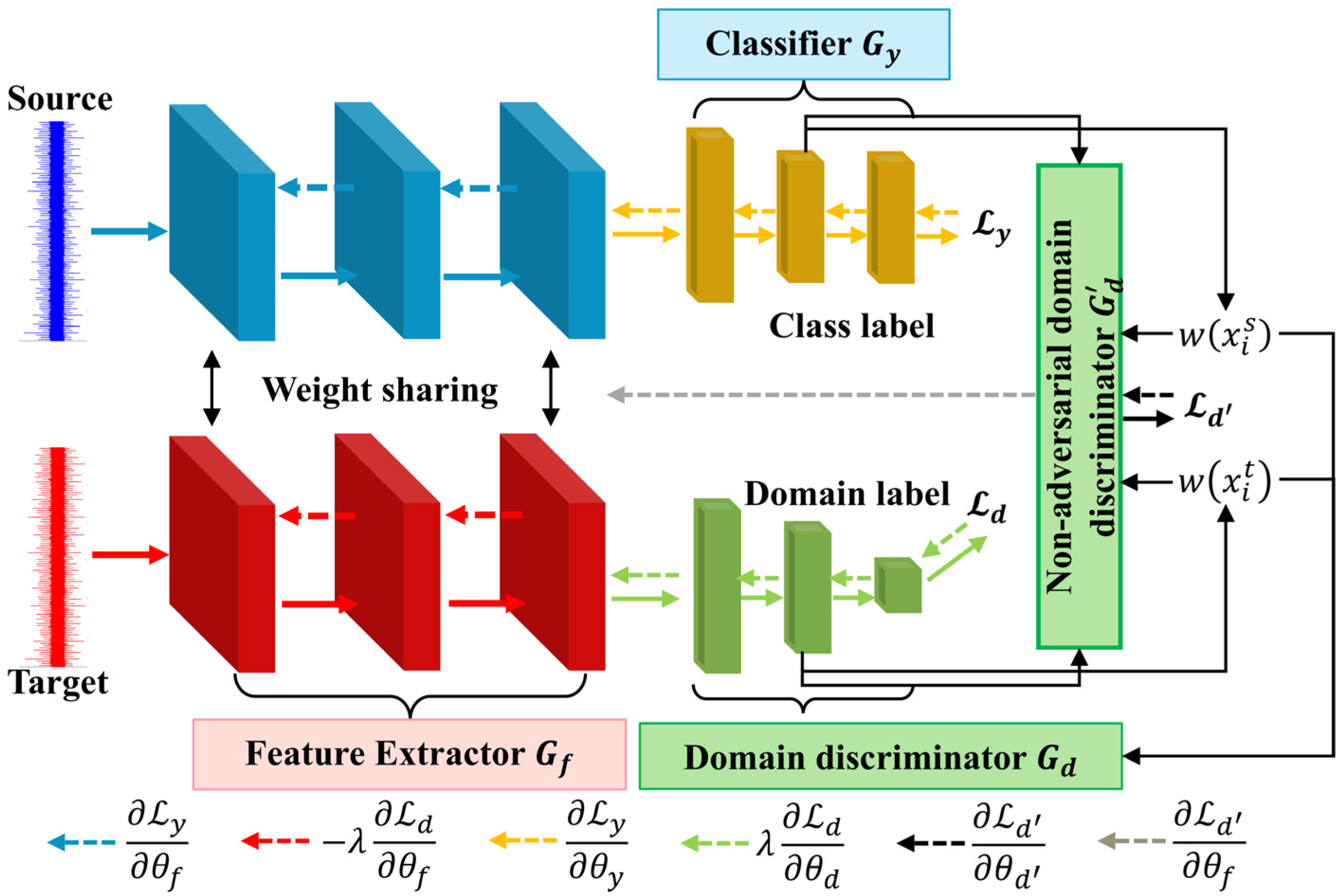
2.3.4. Model Structure and Optimization
3. Experimental Verification
3.1. Case Description
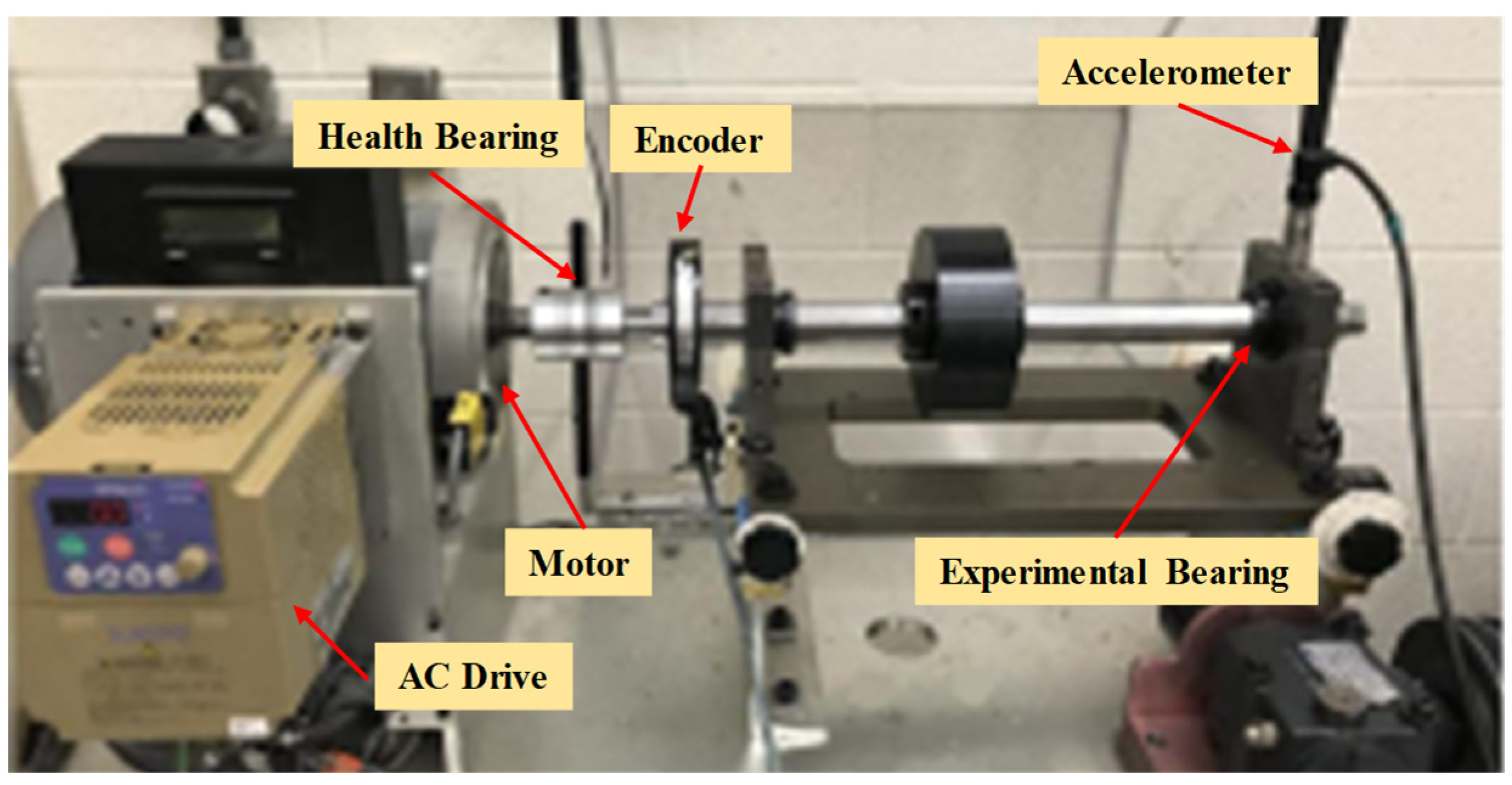
3.1.1. Case Study 1
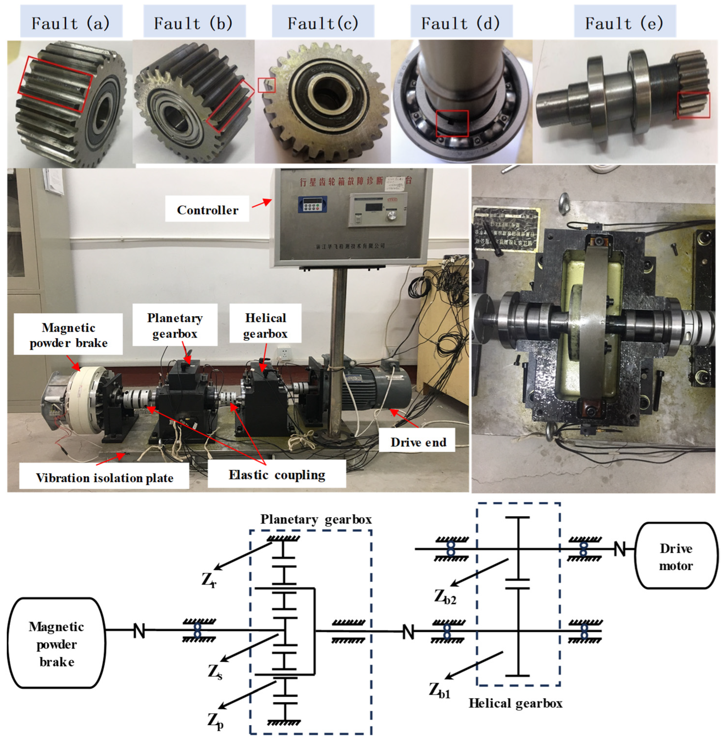
3.1.2. Case Study 2
3.2. Comparison Methods and Implementation Details
3.3. Transferable Feature Extraction Based on Angular Resampling
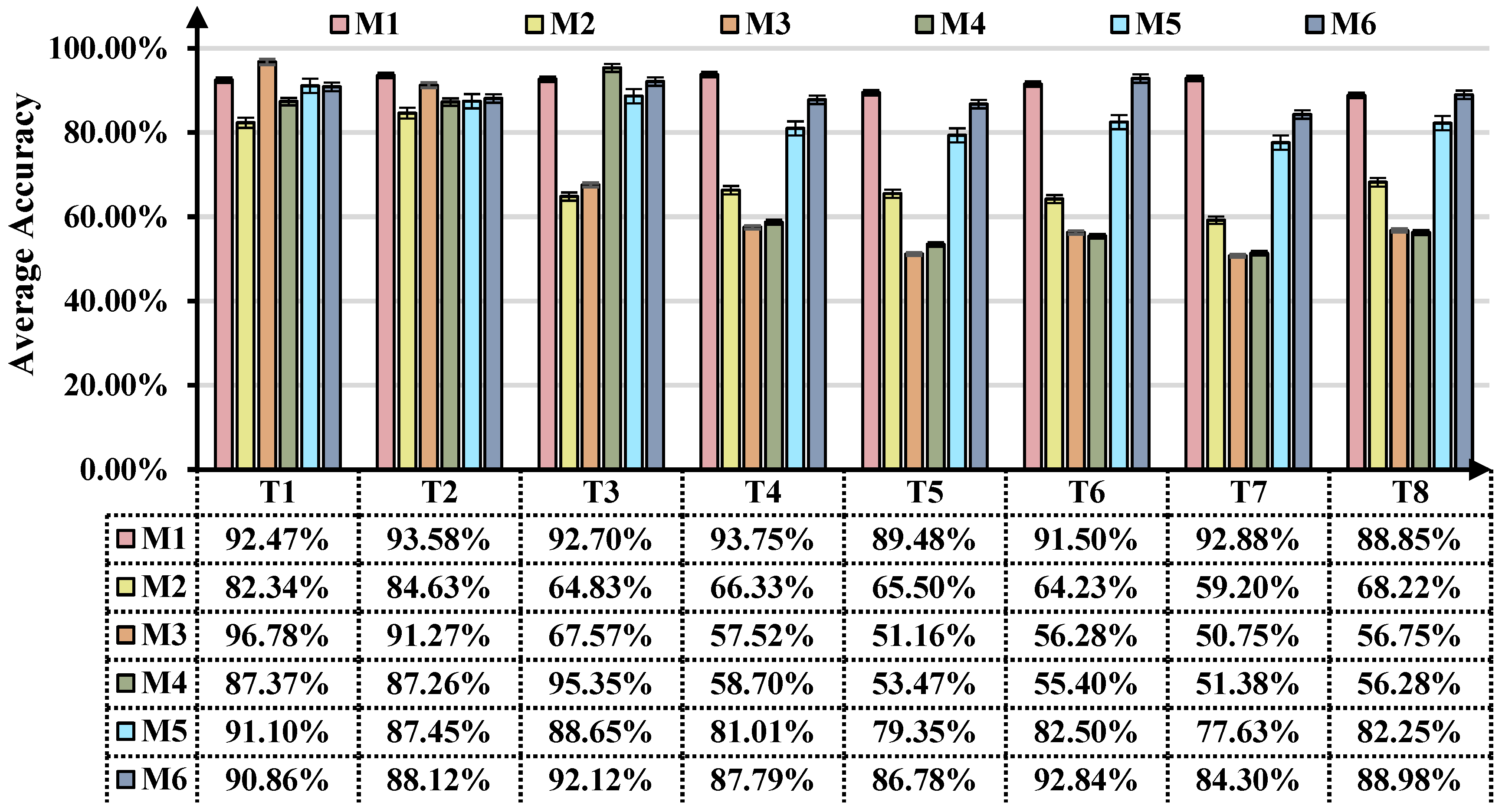
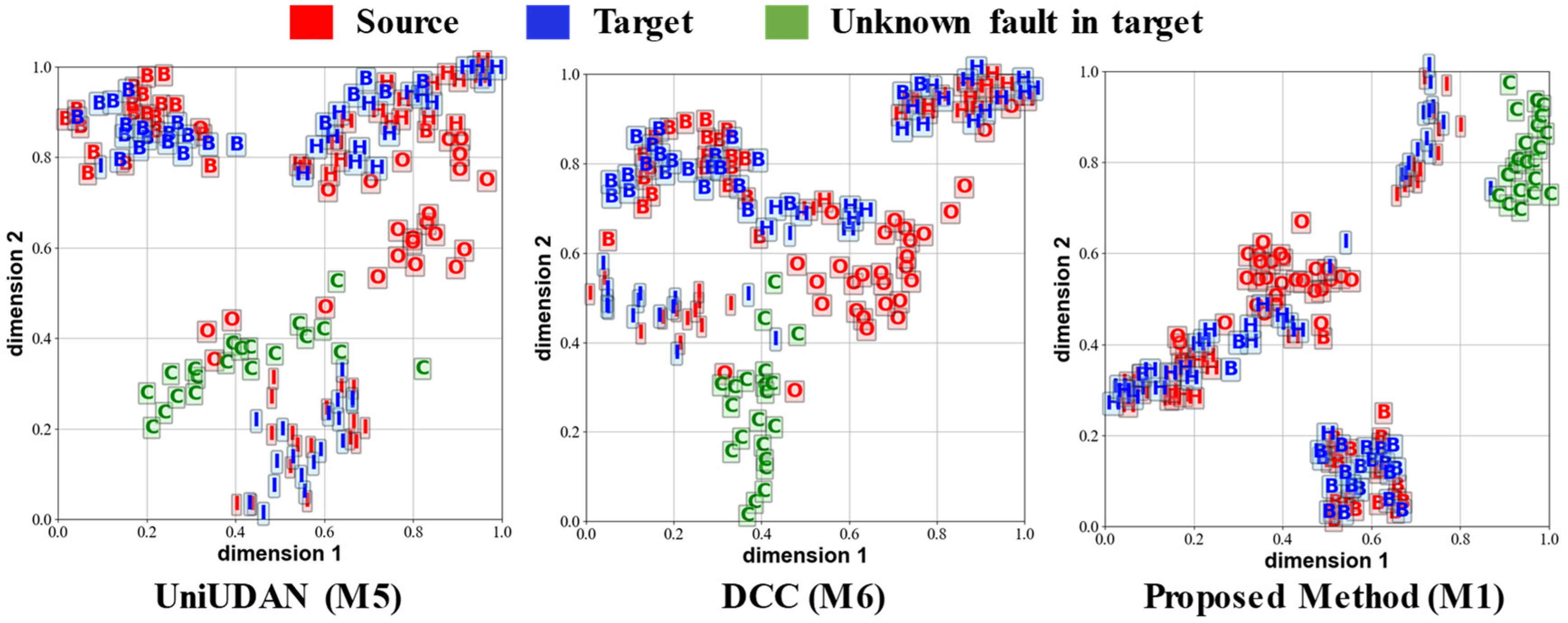
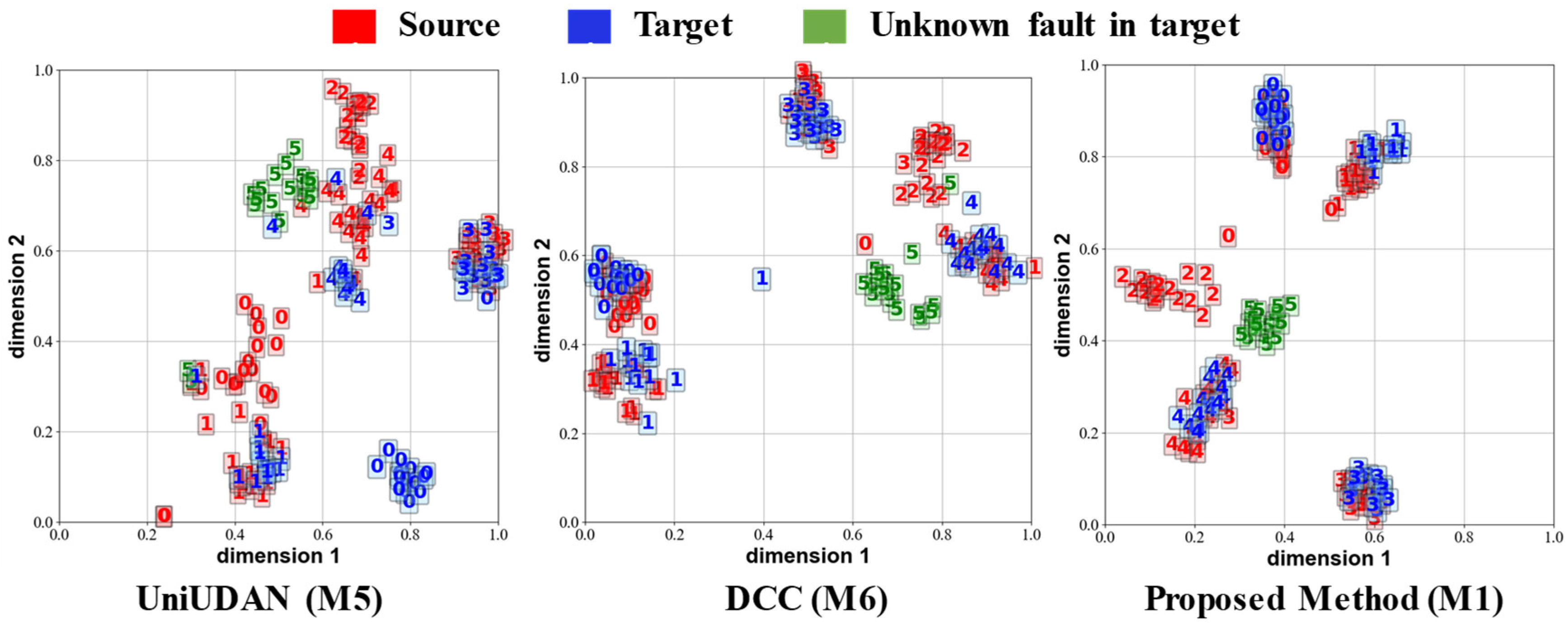
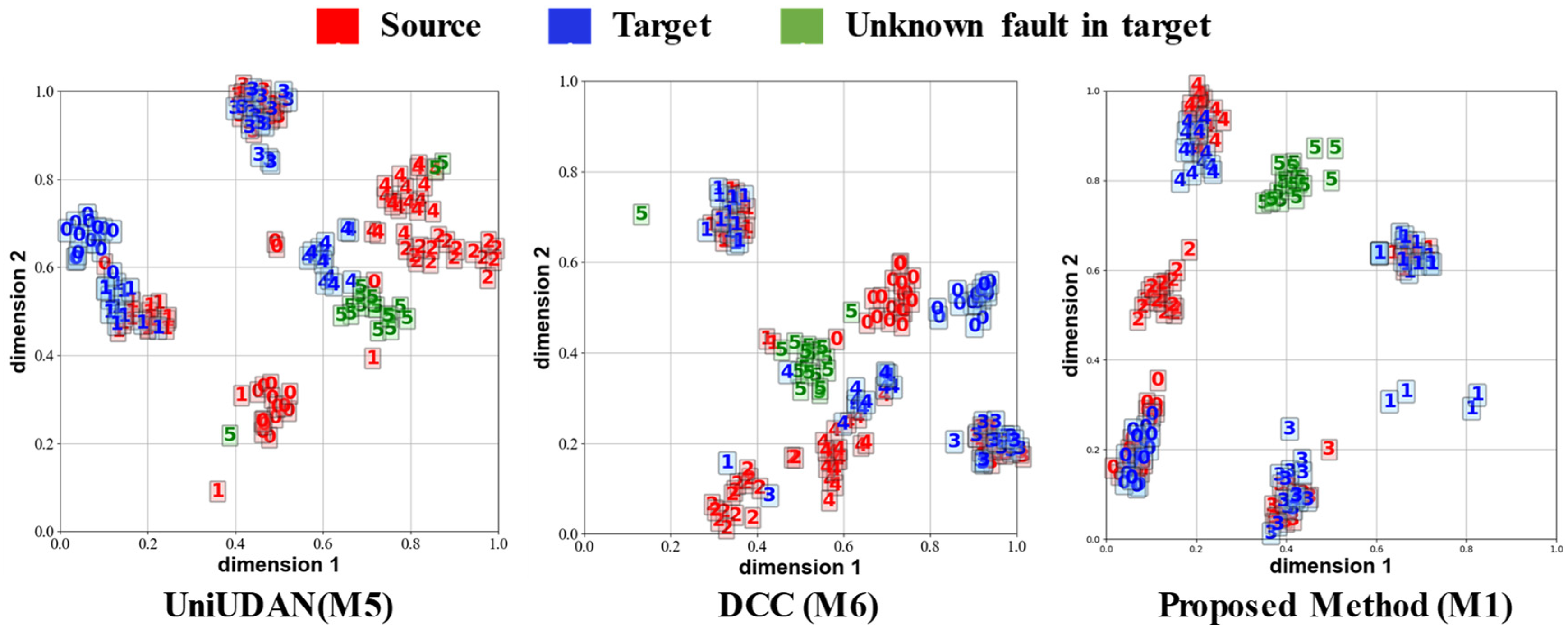
3.4. Diagnostic Accuracy Analysis
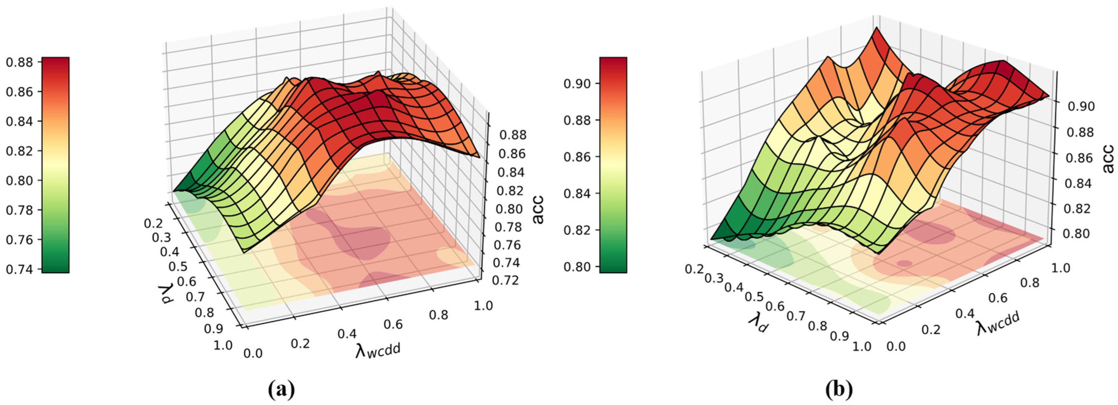
3.5. Parameter Sensitivity Analysis
4. Conclusions
Author Contributions
Funding
Data Availability Statement
Conflicts of Interest
References
- An, Z.; Li, S.; Wang, J.; Jiang, X. A novel bearing intelligent fault diagnosis framework under time-varying working conditions using recurrent neural network. ISA Trans. 2020, 100, 155–170. [Google Scholar] [CrossRef] [PubMed]
- Urbanek, J.; Barszcz, T.; Antoni, J. A two-step procedure for estimation of instantaneous rotational speed with large fluctuations. Mech. Syst. Signal Process. 2013, 38, 96–102. [Google Scholar] [CrossRef]
- Zhao, D.; Li, J.; Cheng, W.; Wen, W. Bearing multi-fault diagnosis with iterative generalized demodulation guided by enhanced rotational frequency matching under time-varying speed conditions. ISA Trans. 2023, 133, 518–528. [Google Scholar] [CrossRef]
- Yang, J.; Yang, C.; Zhuang, X.; Liu, H.; Wang, Z. Unknown bearing fault diagnosis under time-varying speed conditions and strong noise background. Nonlinear Dyn. 2022, 107, 2177–2193. [Google Scholar] [CrossRef]
- Chen, X.; Shu, G.; Zhang, K.; Duan, M.; Li, L. A fault characteristics extraction method for rolling bearing with variable rotational speed using adaptive time-varying comb filtering and order tracking. J. Mech. Sci. Technol. 2022, 36, 1171–1182. [Google Scholar] [CrossRef]
- Hou, F.; Selesnick, I.; Chen, J.; Dong, G. Fault diagnosis for rolling bearings under unknown time-varying speed conditions with sparse representation. J. Sound Vib. 2021, 494, 115854. [Google Scholar] [CrossRef]
- Choudhury, M.D.; Blincoe, K.; Dhupia, J.S. An Overview of Fault Diagnosis of Industrial Machines Operating Under Variable Speeds. Acoust. Aust. 2021, 49, 229–238. [Google Scholar] [CrossRef]
- Han, B.; Ji, S.; Wang, J.; Bao, H.; Jiang, X. An intelligent diagnosis framework for roller bearing fault under speed fluctuation condition. Neurocomputing 2021, 420, 171–180. [Google Scholar] [CrossRef]
- Chen, H.; Luo, H.; Huang, B.; Jiang, B.; Kaynak, O. Transfer Learning-Motivated Intelligent Fault Diagnosis Designs: A Survey, Insights, and Perspectives. IEEE Trans. Neural Netw. Learn. Syst. 2023, 35, 2969–2983. [Google Scholar] [CrossRef]
- Liu, S.; Huang, J.; Ma, J.; Luo, J. SRMANet: Toward an Interpretable Neural Network with Multi-Attention Mechanism for Gearbox Fault Diagnosis. Appl. Sci. 2022, 12, 8388. [Google Scholar] [CrossRef]
- He, D.; Wu, J.; Jin, Z.; Huang, C.G.; Wei, Z.; Yi, C. AGFCN: A bearing fault diagnosis method for high-speed train bogie under complex working conditions. Reliab. Eng. Syst. Saf. 2025, 258, 110907. [Google Scholar] [CrossRef]
- Zheng, H.; Yang, Y.; Yin, J.; Li, Y.; Wang, R.; Xu, M. Deep Domain Generalization Combining A Priori Diagnosis Knowledge Toward Cross-Domain Fault Diagnosis of Rolling Bearing. IEEE Trans. Instrum. Meas. 2021, 70, 1–11. [Google Scholar] [CrossRef]
- Liu, J.; Cao, H.; Su, S.; Chen, X. Simulation-Driven Subdomain Adaptation Network for bearing fault diagnosis with missing samples. Eng. Appl. Artif. Intell. 2023, 123, 106201. [Google Scholar] [CrossRef]
- Li, X.; Li, S.; Wei, D.; Si, L.; Yu, K.; Yan, K. Dynamics simulation-driven fault diagnosis of rolling bearings using security transfer support matrix machine. Reliab. Eng. Syst. Saf. 2024, 243, 109882. [Google Scholar] [CrossRef]
- Zhao, C.; Zio, E.; Shen, W. Domain generalization for cross-domain fault diagnosis: An application-oriented perspective and a benchmark study. Reliab. Eng. Syst. Saf. 2024, 245, 109964. [Google Scholar] [CrossRef]
- Long, M.; Zhu, H.; Wang, J.; Jordan, M.I. Deep Transfer Learning with Joint Adaptation Networks. In Proceedings of the 34th International Conference on Machine Learning, PMLR, Sydney, Australia, 6–11 August 2017; Volume 70, pp. 2208–2217. [Google Scholar]
- Sun, B.; Saenko, K. Deep CORAL: Correlation Alignment for Deep Domain Adaptation. In Computer Vision–ECCV 2016 Workshops; Hua, G., Jégou, H., Eds.; Springer International Publishing: Cham, Switzerland, 2016; pp. 443–450. [Google Scholar] [CrossRef]
- Zhu, Y.; Zhuang, F.; Wang, J.; Ke, G.; Chen, J.; Bian, J.; Xiong, H.; He, Q. Deep Subdomain Adaptation Network for Image Classification. IEEE Trans. Neural Netw. Learn. Syst. 2021, 32, 1713–1722. [Google Scholar] [CrossRef] [PubMed]
- Ganin, Y.; Ustinova, E.; Ajakan, H.; Germain, P.; Larochelle, H.; Laviolette, F.; Marchand, M.; Lempitsky, V. Domain-Adversarial Training of Neural Networks. In Domain-Adversarial Training of Neural Networks; Csurka, G., Ed.; Springer International Publishing: Cham, Switzerland, 2017; pp. 189–209. [Google Scholar] [CrossRef]
- Long, M.; Cao, Z.; Wang, J.; Jordan, M.I. Conditional Adversarial Domain Adaptation. arXiv 2018, arXiv:170510667. Available online: http://arxiv.org/abs/1705.10667 (accessed on 2 December 2021).
- Li, J.; Chen, E.; Ding, Z.; Zhu, L.; Lu, K.; Shen, H.T. Maximum Density Divergence for Domain Adaptation. IEEE Trans. Pattern Anal. Mach. Intell. 2021, 43, 3918–3930. [Google Scholar] [CrossRef]
- Li, X.; Jia, X.-D.; Zhang, W.; Ma, H.; Luo, Z.; Li, X. Intelligent cross-machine fault diagnosis approach with deep auto-encoder and domain adaptation. Neurocomputing 2020, 383, 235–247. [Google Scholar] [CrossRef]
- Jiao, J.; Zhao, M.; Lin, J.; Liang, K. Residual joint adaptation adversarial network for intelligent transfer fault diagnosis. Mech. Syst. Signal Process. 2020, 145, 106962. [Google Scholar] [CrossRef]
- Zhou, H.; Huang, X.; Wen, G.; Dong, S.; Lei, Z.; Zhang, P.; Chen, X. Convolution enabled transformer via random contrastive regularization for rotating machinery diagnosis under time-varying working conditions. Mech. Syst. Signal Process. 2022, 173, 109050. [Google Scholar] [CrossRef]
- Li, W.; Huang, R.; Li, J.; Liao, Y.; Chen, Z.; He, G.; Yan, R.; Gryllias, K. A perspective survey on deep transfer learning for fault diagnosis in industrial scenarios: Theories, applications and challenges. Mech. Syst. Signal Process. 2022, 167, 108487. [Google Scholar] [CrossRef]
- Xiao, Y.; Zhou, X.; Zhou, H.; Wang, J. Multi-label deep transfer learning method for coupling fault diagnosis. Mech. Syst. Signal Process. 2024, 212, 111327. [Google Scholar] [CrossRef]
- Liu, S.; Huang, J.; Ma, J.; Jing, L.; Wang, Y. Complementary-label adversarial domain adaptation fault diagnosis network under time-varying rotational speed and weakly-supervised conditions. Comput. Mater. Contin. 2024, 79, 839–850. [Google Scholar] [CrossRef]
- Hospedales, T.; Antoniou, A.; Micaelli, P.; Storkey, A. Meta-Learning in Neural Networks: A Survey. IEEE Trans. Pattern Anal. Mach. Intell. 2022, 44, 5149–5169. [Google Scholar] [CrossRef]
- Xian, Y.; Schiele, B.; Akata, Z. Zero-Shot Learning—The Good, the Bad and the Ugly. In Proceedings of the 2017 IEEE Conference on Computer Vision and Pattern Recognition (CVPR), Honolulu, HI, USA, 21–26 July 2017; pp. 3077–3086. [Google Scholar] [CrossRef]
- Vinyals, O.; Blundell, C.; Lillicrap, T.; Kavukcuoglu, K.; Wierstra, D. Matching Networks for One Shot Learning. In Proceedings of the 30th International Conference on Neural Information Processing Systems, Barcelona, Spain, 5–10 December 2016; Curran Associates Inc.: Red Hook, NY, USA, 2016; pp. 3637–3645. [Google Scholar]
- Zhao, Z.; Zhang, Q.; Yu, X.; Sun, C.; Wang, S.; Yan, R.; Chen, X. Applications of Unsupervised Deep Transfer Learning to Intelligent Fault Diagnosis: A Survey and Comparative Study. IEEE Trans. Instrum. Meas. 2021, 70, 3525828. [Google Scholar] [CrossRef]
- Zhang, W.; Li, X.; Ma, H.; Luo, Z.; Li, X. Open-Set Domain Adaptation in Machinery Fault Diagnostics Using Instance-Level Weighted Adversarial Learning. IEEE Trans. Ind. Inform. 2021, 17, 7445–7455. [Google Scholar] [CrossRef]
- Zhang, W.; Li, X.; Ma, H.; Luo, Z.; Li, X. Universal Domain Adaptation in Fault Diagnostics with Hybrid Weighted Deep Adversarial Learning. IEEE Trans. Ind. Inform. 2021, 17, 7957–7967. [Google Scholar] [CrossRef]
- Yang, B.; Xu, S.; Lei, Y.; Lee, C.-G.; Stewart, E.; Roberts, C. Multi-source transfer learning network to complement knowledge for intelligent diagnosis of machines with unseen faults. Mech. Syst. Signal Process. 2022, 162, 108095. [Google Scholar] [CrossRef]
- You, K.; Long, M.; Cao, Z.; Wang, J.; Jordan, M.I. Universal Domain Adaptation. In Proceedings of the 2019 IEEE/CVF Conference on Computer Vision and Pattern Recognition (CVPR), Long Beach, CA, USA, 15–20 June 2019; pp. 2715–2724. [Google Scholar] [CrossRef]
- Huang, H.; Baddour, N. Bearing vibration data collected under time-varying rotational speed conditions. Data Brief 2018, 21, 1745–1749. [Google Scholar] [CrossRef]
- Liu, X.; Guo, Z.; Li, S.; Xing, F.; You, J.; Kuo, C.-C.J.; El Fakhri, G.; Woo, J. Adversarial Unsupervised Domain Adaptation with Conditional and Label Shift: Infer, Align and Iterate. In Proceedings of the 2021 IEEE/CVF International Conference on Computer Vision (ICCV), Montreal, QC, Canada, 10–17 October 2021; pp. 10347–10356. [Google Scholar] [CrossRef]
- Zhang, D.; Feng, Z. Enhancement of adaptive mode decomposition via angular resampling for nonstationary signal analysis of rotating machinery: Principle and applications. Mech. Syst. Signal Process. 2021, 160, 107909. [Google Scholar] [CrossRef]
- Villa, L.F.; Reñones, A.; Perán, J.R.; de Miguel, L.J. Angular resampling for vibration analysis in wind turbines under non-linear speed fluctuation. Mech. Syst. Signal Process. 2011, 25, 2157–2168. [Google Scholar] [CrossRef]
- Yin, Y.; Yang, Z.; Wu, X.; Hu, H. Unveiling Class-Labeling Structure for Universal Domain Adaptation. arXiv 2020, arXiv:2010.04873. [Google Scholar]
- Kang, G.; Jiang, L.; Yang, Y.; Hauptmann, A.G. Contrastive Adaptation Network for Unsupervised Domain Adaptation. In Proceedings of the 2019 IEEE/CVF Conference on Computer Vision and Pattern Recognition (CVPR), Long Beach, CA, USA, 15–20 June 2019; pp. 4888–4897. [Google Scholar] [CrossRef]
- Li, G.; Kang, G.; Zhu, Y.; Wei, Y.; Yang, Y. Domain Consensus Clustering for Universal Domain Adaptation. In Proceedings of the 2021 IEEE/CVF Conference on Computer Vision and Pattern Recognition (CVPR), Nashville, TN, USA, 20–25 June 2021; pp. 9752–9761. [Google Scholar] [CrossRef]
- Hassan, E.; Shams, M.Y.; Hikal, N.A.; Elmougy, S. The effect of choosing optimizer algorithms to improve computer vision tasks: A comparative study. Multimed. Tools Appl. 2023, 82, 16591–16633. [Google Scholar] [CrossRef] [PubMed]
- Saito, K.; Yamamoto, S.; Ushiku, Y.; Harada, T. Open set domain adaptation by backpropagation. In Proceedings of the European Conference on Computer Vision (ECCV), Munich, Germany, 8–14 September 2018; pp. 153–168. [Google Scholar]


| Task | Source Class (Inconsistent Speed Fluctuation of A, B, C, D) | Source Speed Varying Conditions | Target Class (Inconsistent Speed Fluctuation of A, B, C, D) | Target Speed Varying Conditions | DA Scenario |
|---|---|---|---|---|---|
| O1 | HA, IA, OA, BA, CA | IS | HB, IB, OB, BB, CB | DS | CUDA |
| O2 | HA, IA, OA, BA, CA | IS | HB, IB, OB, BB | DS | PUDA |
| O3 | HA, IA, OA, BA | IS | HB, IB, OB, BB, CB | DS | OSUDA |
| O4 | HA, OA, BA, CA | IS | HB, IB, OB, BB | DS | UniUDA |
| O5 | HA, OA, BA | IS | HB, IB, BB, CB | DS | UniUDA |
| O6 | HB, IB, OB, BB | DS | HC, IC, BC, CC | IS then DS | UniUDA |
| O7 | HB, OB, BB | DS | HC, IC, CC | IS then DS | UniUDA |
| O8 | HC, IC, OC, BC | IS then DS | HD, ID, BD, CD | DS then IS | UniUDA |
| Task | Source Class (A: Load = 0.5 A; B: Load = 1 A) | Source Speed Varying Conditions | Target Class (A: Load = 0.5 A; B: Load = 1 A) | Target Speed Varying Conditions | DA Scenario |
|---|---|---|---|---|---|
| T1 | HA1, CA1, IA1, WA1, KA1, PA1 | IS | HA2, CA2, IA2, WA2, KA2, PA2 | IS | CUDA |
| T2 | HA1, CA1, IA1, WA1, KA1, PA1 | IS | HA2, CA2, IA2, WA2, KA2 | IS | PUDA |
| T3 | HA1, CA1, WA1, KA1, PA1 | IS | HA2, CA2, IA2, WA2, KA2, PA2 | IS | OSUDA |
| T4 | HA1, CA1, WA1, KA1, PA1 | IS | HA2, CA2, IA2, WA2, KA2 | IS | UniUDA |
| T5 | HA1, CA1, KA1, PA1 | IS | HA2, CA2, IA2, WA2 | IS | UniUDA |
| T6 | HB1, CB1, KB1, PB1 | DS | HB2, CB2, IB2, WB2 | DS | UniUDA |
| T7 | HA1, CA1, IA1, WA1, KA1 | IS | HB1, CB1, WB1, KB1, PB1 | DS | UniUDA |
| T8 | HA2, CA2, KA2, PA2 | IS | HB2, CB2, IB2, WB2, | DS | UniUDA |
Disclaimer/Publisher’s Note: The statements, opinions and data contained in all publications are solely those of the individual author(s) and contributor(s) and not of MDPI and/or the editor(s). MDPI and/or the editor(s) disclaim responsibility for any injury to people or property resulting from any ideas, methods, instructions or products referred to in the content. |
© 2025 by the authors. Licensee MDPI, Basel, Switzerland. This article is an open access article distributed under the terms and conditions of the Creative Commons Attribution (CC BY) license (https://creativecommons.org/licenses/by/4.0/).
Share and Cite
Liu, S.; Huang, J.; Han, P.; Fan, Z.; Ma, J. Cross-Domain Fault Diagnosis of Rotating Machinery Under Time-Varying Rotational Speed and Asymmetric Domain Label Condition. Sensors 2025, 25, 2818. https://doi.org/10.3390/s25092818
Liu S, Huang J, Han P, Fan Z, Ma J. Cross-Domain Fault Diagnosis of Rotating Machinery Under Time-Varying Rotational Speed and Asymmetric Domain Label Condition. Sensors. 2025; 25(9):2818. https://doi.org/10.3390/s25092818
Chicago/Turabian StyleLiu, Siyuan, Jinying Huang, Peiyu Han, Zhenfang Fan, and Jiancheng Ma. 2025. "Cross-Domain Fault Diagnosis of Rotating Machinery Under Time-Varying Rotational Speed and Asymmetric Domain Label Condition" Sensors 25, no. 9: 2818. https://doi.org/10.3390/s25092818
APA StyleLiu, S., Huang, J., Han, P., Fan, Z., & Ma, J. (2025). Cross-Domain Fault Diagnosis of Rotating Machinery Under Time-Varying Rotational Speed and Asymmetric Domain Label Condition. Sensors, 25(9), 2818. https://doi.org/10.3390/s25092818