
Centralized Measurement Level Fusion of GNSS and Inertial Sensors for Robust Positioning and Navigation

 ,
,  , ,
, ,  and
and 
Abstract
1. Introduction
- It allows for the continuous surveillance and monitoring of assets and resources. This integration can be used to optimize operations, increase efficiency, and reduce costs in industries such as logistics, supply chain management, and transportation. Companies, for example, may properly track shipments in real-time, monitor routes, and ensure timely deliveries by equipping delivery vehicles with cellphones equipped with a GNSS/INS [2].
- Context-aware services and personalized experiences are made possible by the integration of GNSS/INS in smartphones. Location-based applications can employ exact positioning data to deliver personalized suggestions, local information, and targeted adverts to users. This technology supports smart city projects by providing real-time information on transport, parking availability, surrounding amenities, and cultural events to city people, encouraging a more connected and comfortable urban lifestyle [8,9].
- It improves the safety and security of the IoT ecosystem. Emergency response systems can quickly detect and assist persons in need during critical situations by correctly determining the position and motions of humans and assets. In addition, IoT-enabled security systems can benefit from smartphones with a GNSS/INS, which provide exact geolocation for tracing stolen devices, guarding restricted areas, and assuring human safety [10].
1.1. Objectives
- The application of satellite selection-based MDDA to both LC and TC algorithms for all visible satellites.
- The application of the proposed algorithm in scenarios where the receiver is limited to a specific number of channels.
- The analysis of the impact of the selected satellite-based MDDA on the overall positioning performance.
1.2. Paper Organization
2. Related Work
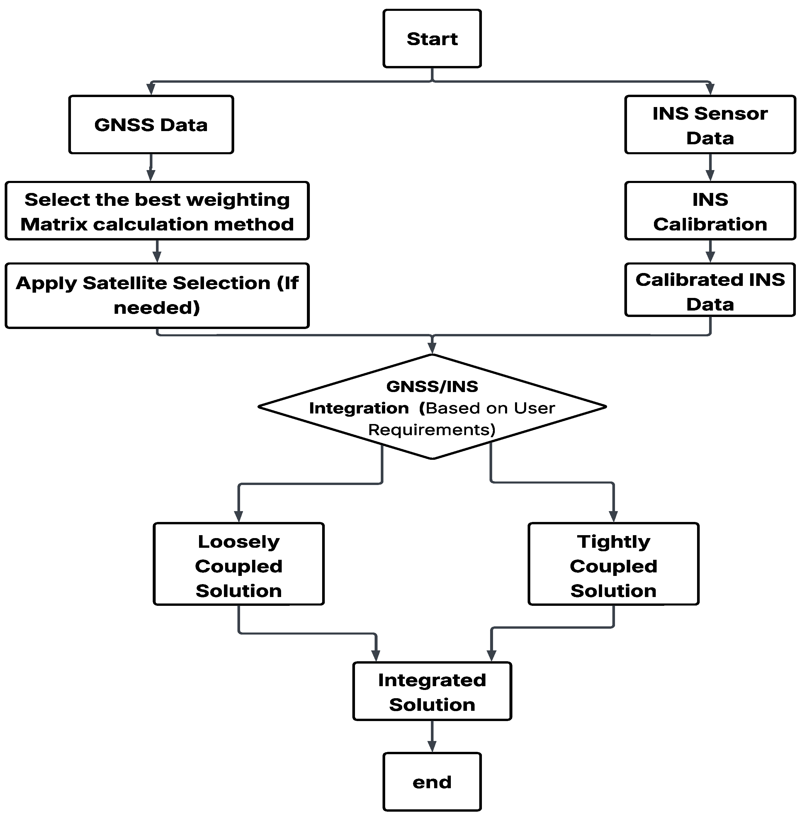
3. Methodology
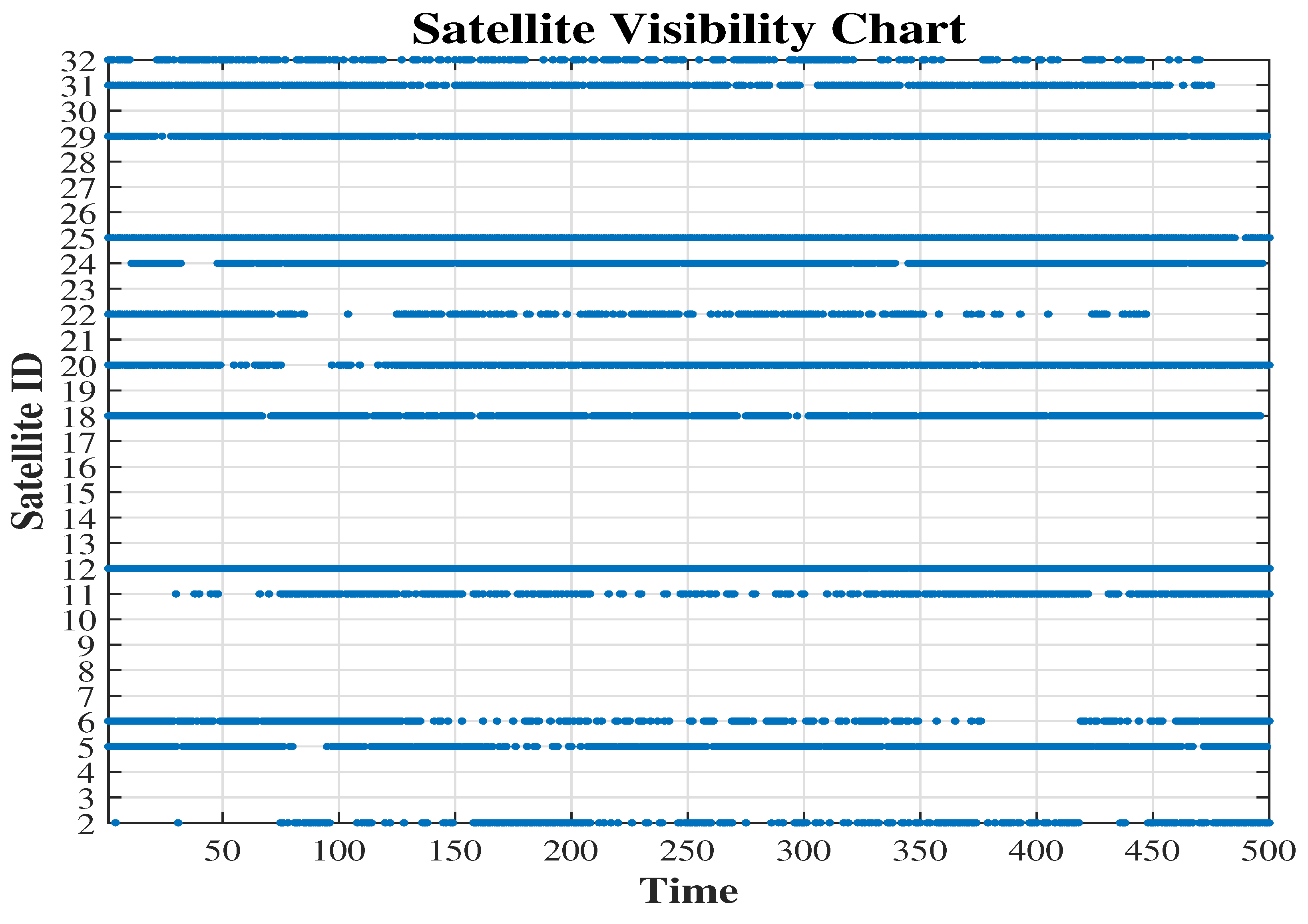
3.1. Data Recording and Analysis
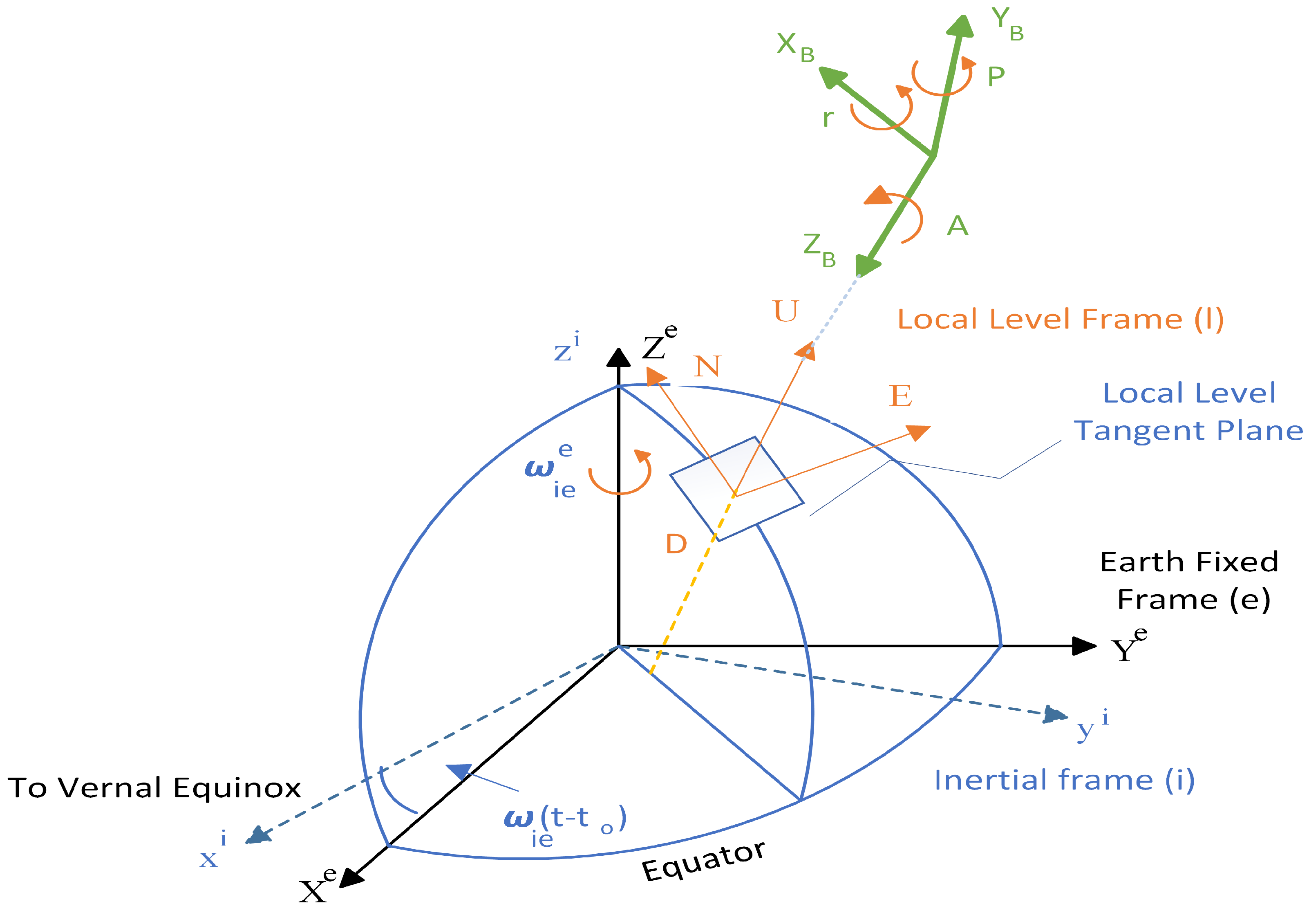
3.2. Coordinate Frames
3.3. Traditional Weighting Matrix Model
- Carrier to noise density-based model ( model): In [35,36], the model was structured around the signal-to-noise ratio , expressed as follows:where b is constantly defined empirically and equals . In [12,38,39], the proposed standard deviation of code observationIn this context, the coefficient a represents the root mean square value (RMS) of pseudorange observation residuals, while b corresponds to the pseudorange coarse acquisition (C/A-code) chipping length, which was defined as 293 m for L1 measurements.
- -model: In [35,37,40,41], a combination model was proposed that depended on both and :where k is 1 if the line-of-sight (LOS) signal is available and 2 or ∞ if no LOS signal is available:where x, y, and z model a nonlinear regression problem that relates the mean of Inverse-Gamma estimated distributions and the corresponding pair [40].
- Google proposed sigma: In the smartphone’s RGNSSM, there is a provided value referred to as Received Space Vehicle Time Uncertainty Nanos (RSVTUN). This value signifies the estimated discrepancy in the received GNSS time.Google advises filling the weighting matrix with this value, yet neither the Android developer’s guide nor the accompanying white paper offers guidance on its calculation [16].
3.4. Satellite Selection (SS) Techniques
- Based on : In [44], a fuzzy SS algorithm was utilized to select a set of satellites with the highest and minimum geometrical dilution of precision (GDOP).
- Brute force (optimal) method: Through the process of evaluating all possible combinations and selecting the optimal performance set, this approach ensures the best performance. However, it comes with the drawback of high computational cost [43].Given n satellites on the horizon and a receiver with k channels, the set of available options for the optimal method, denoted as , is determined byFor example, if n = 30 and k = 25, 142,506 geometries should be evaluated.
- Greedy method: Similar to the optimal method for evaluating subset performance, this approach removes only one satellite at a time and utilizes the determined geometry to calculate the next iteration [43,45].The numbers of are given byFor example, if n = 30 and k = 25, then the number of geometries to evaluate is reduced to 140.
- Downdate method: Given our objective to optimize elements of the covariance matrix, we revert to employing the greedy algorithm approach. The position covariance matrix (CM) in the north–east–down (NED) frame is used:where G is the geometry matrix in the NED frame and R is the weighting matrix.To find the best subset, the CM must be calculated in Equation (12):where is the position CM with the removed satellite and is the S matrix column.Although the downdate method suggests a more efficient way to implement the greedy algorithm, it also provides insights into an even more efficient algorithm. By examining Equation (12), we can observe this potential improvement.The rise in CM will manifest in the final term of Equation (15). The smaller this term, the less impact it will have on increasing the corresponding covariation term.To obtain the best subset, one can sort the values in Equation (16) from all calculations and then retain the largest values of this cost function [43,46].This method outperforms the greedy approach. Similar to the EL-based method, it involves calculating a set of all in-view solutions initially and then selecting the optimal subset.
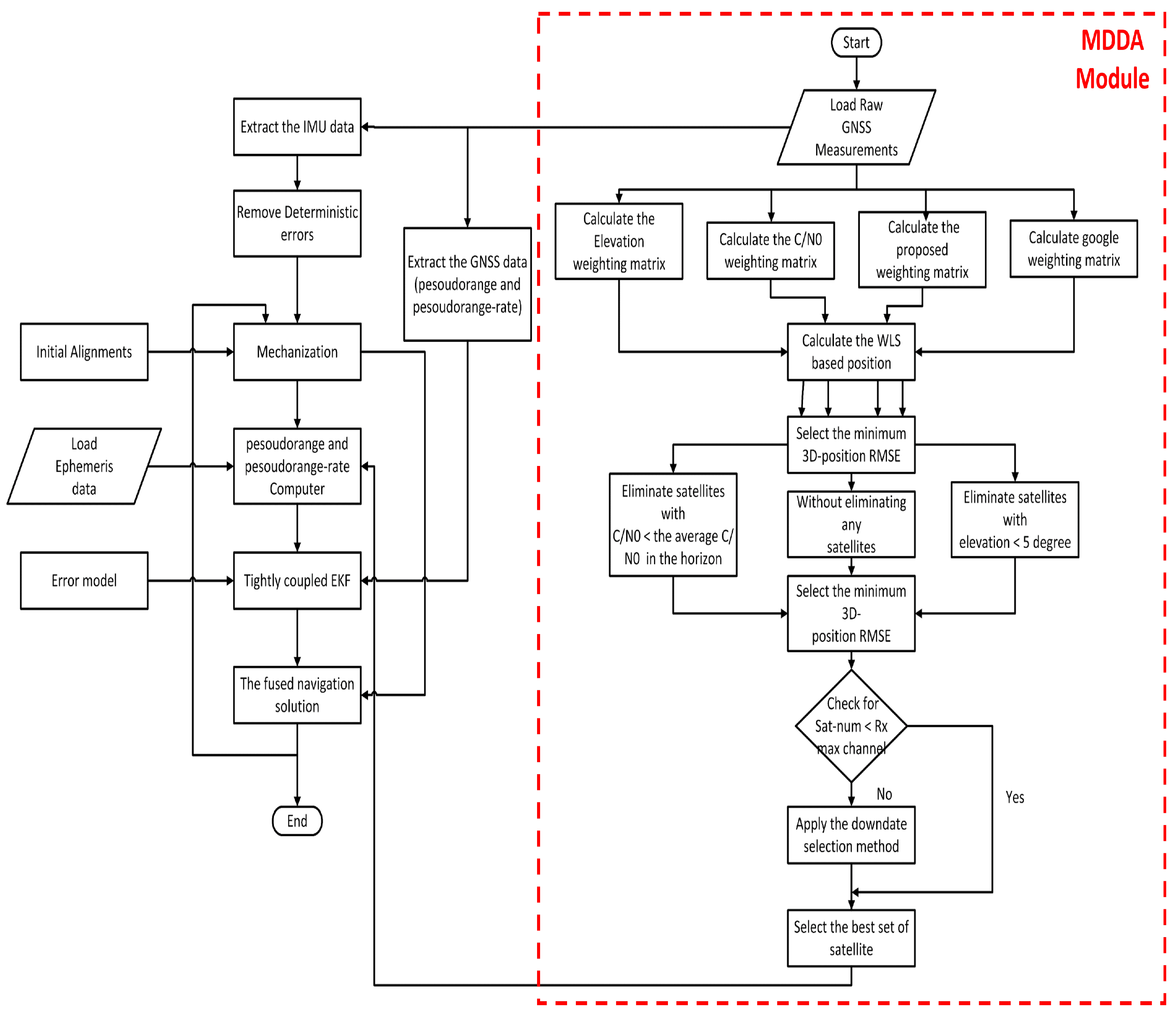
3.5. The Proposed MDDA Algorithm
3.6. MDDA Augmented GNSS/INS Integration
3.6.1. IMU Calibration
3.6.2. INS Mechanization
- The singularity issue that can occur when using Euler angles is avoided by the quaternion solution.
- It is rather easy to execute the quaternion computation.
- Instead of six differential equations if directions cosines are used, just four equations are numerically solved.
3.6.3. Extended Kalman Filter (EKF)
3.6.4. Error Model
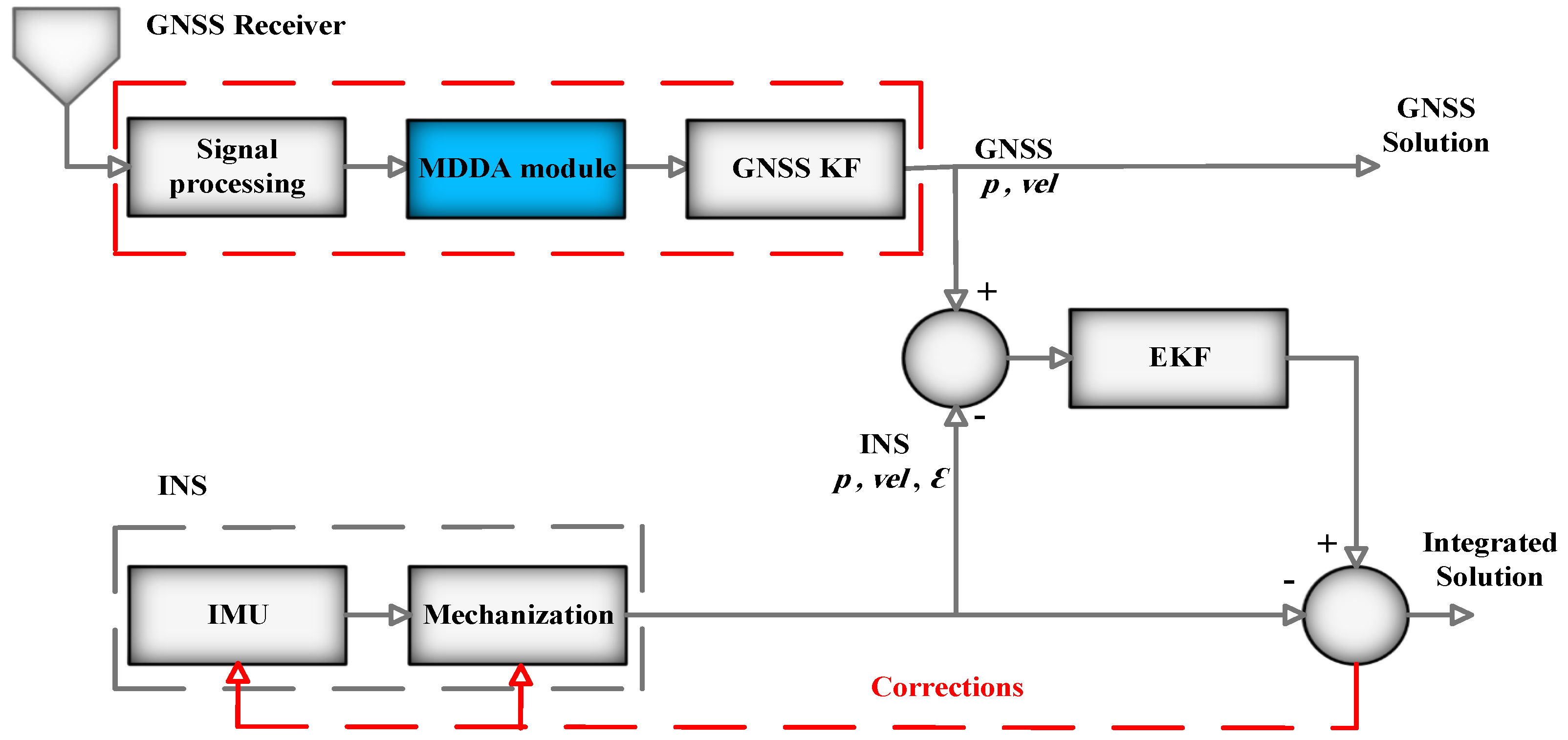
3.6.5. LC Integration Model
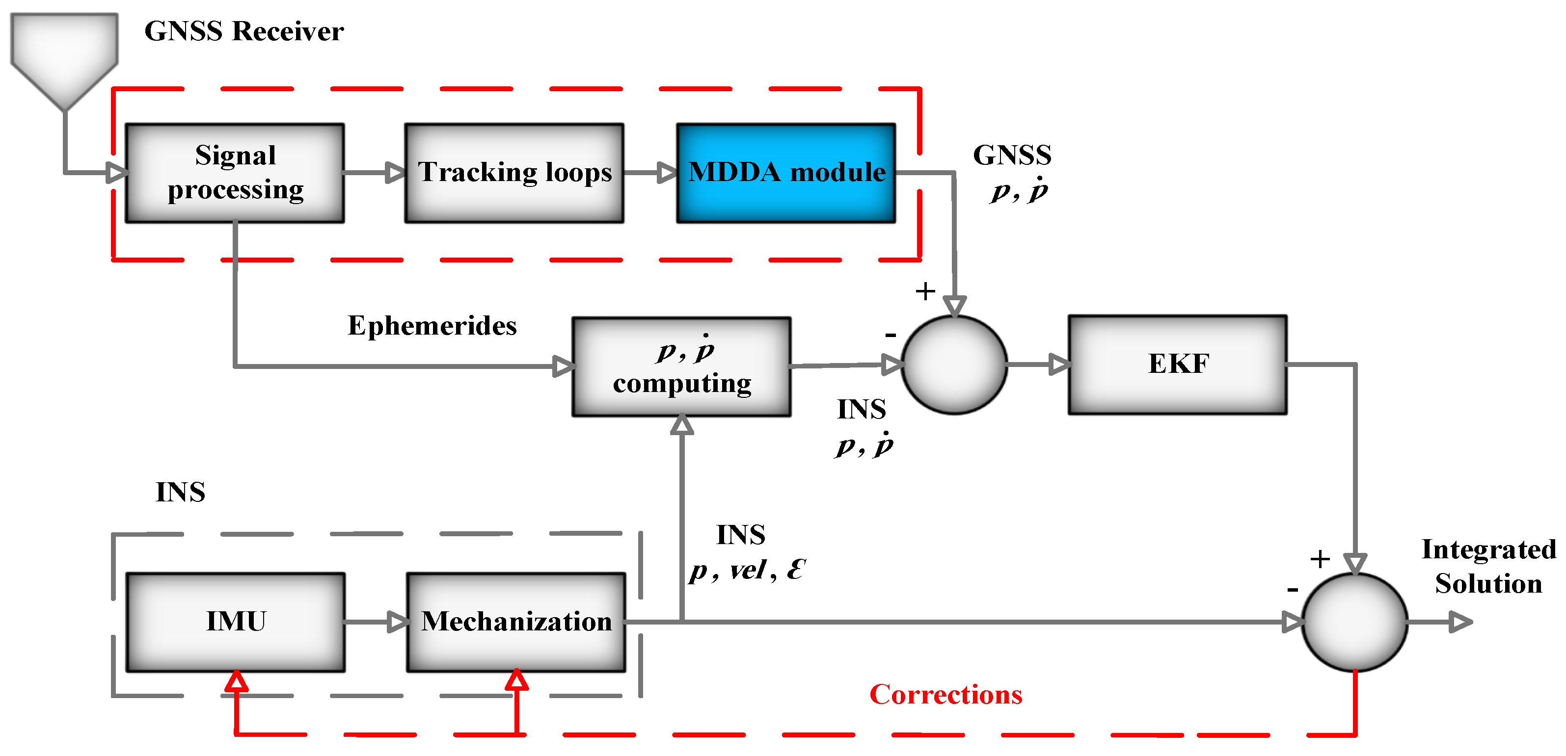
3.6.6. TC Integration Model
4. Experimental Setup
5. Results and Discussion
- MDDA was applied to all visible satellites and processed exclusively by the receiver.
- MDDA was integrated into the LC architecture to enhance its overall performance.
- MDDA was also incorporated into the TC architecture to further optimize performance.
- Lastly, all these scenarios were assessed while taking into account the additional constraints posed by restricted receiver channels.
5.1. MDDA with Receiver-Only Scenario
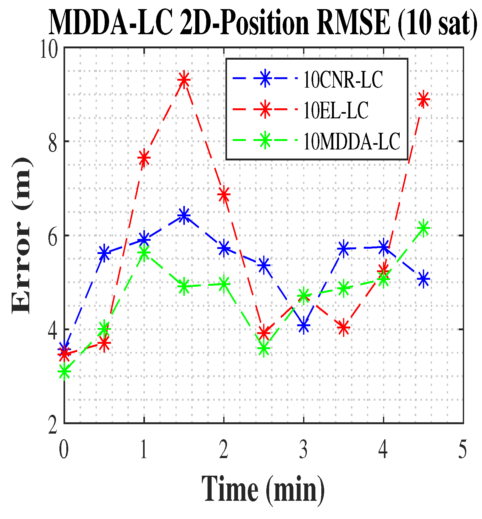
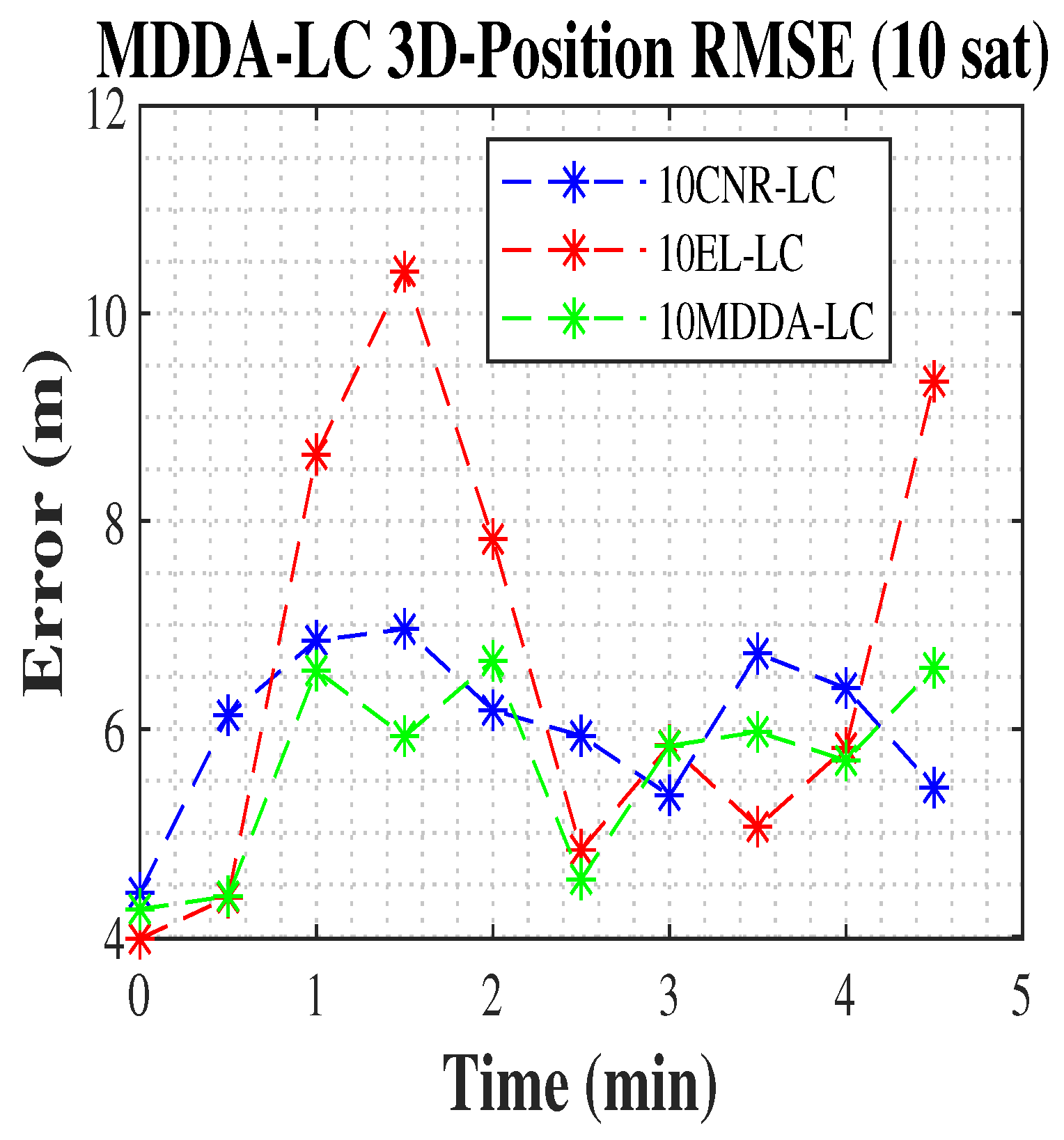
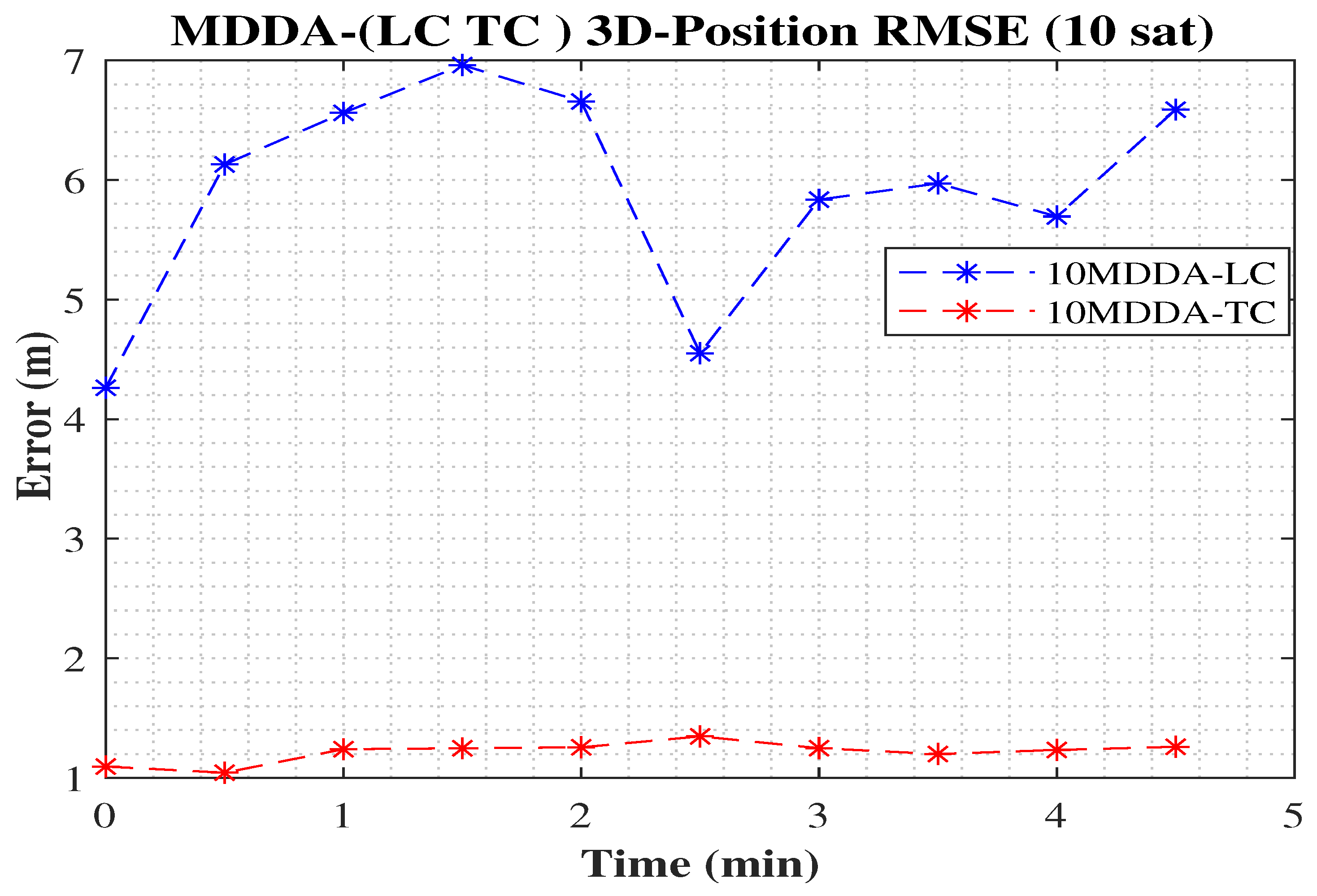
5.2. MDDA with LC Integration Scenario
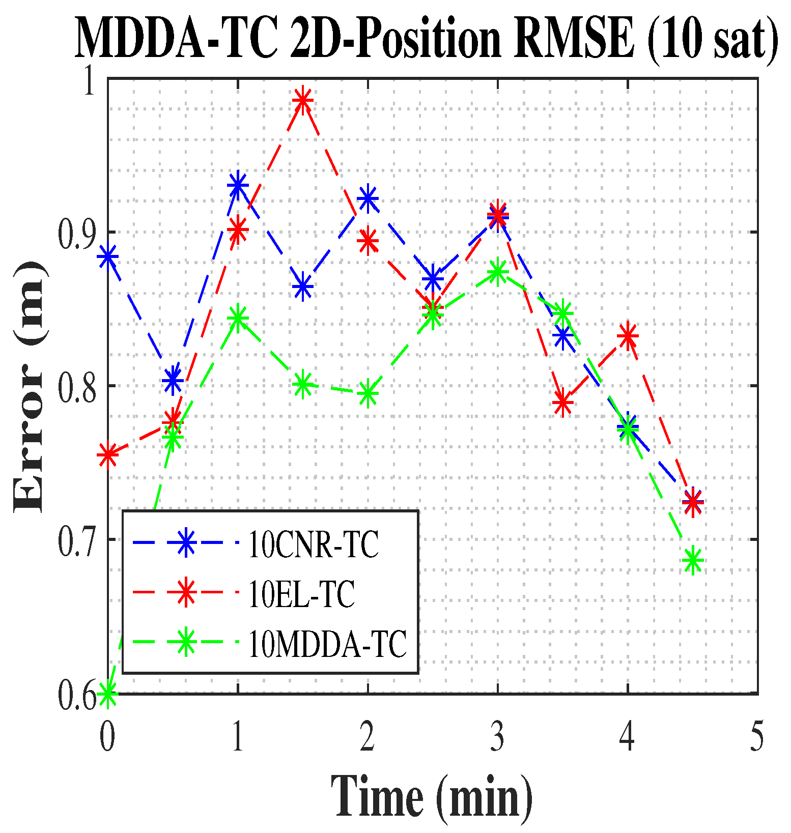
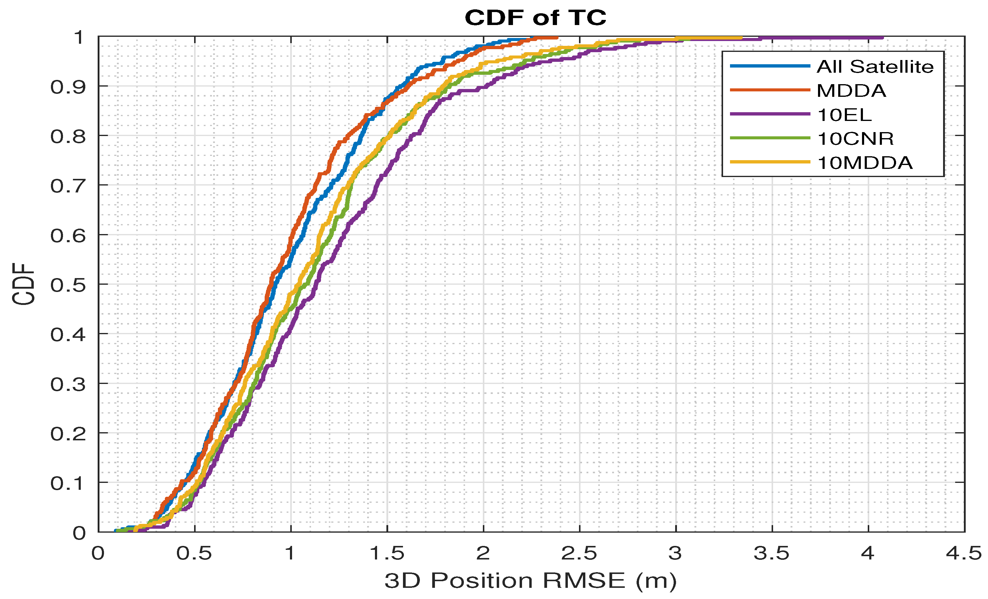
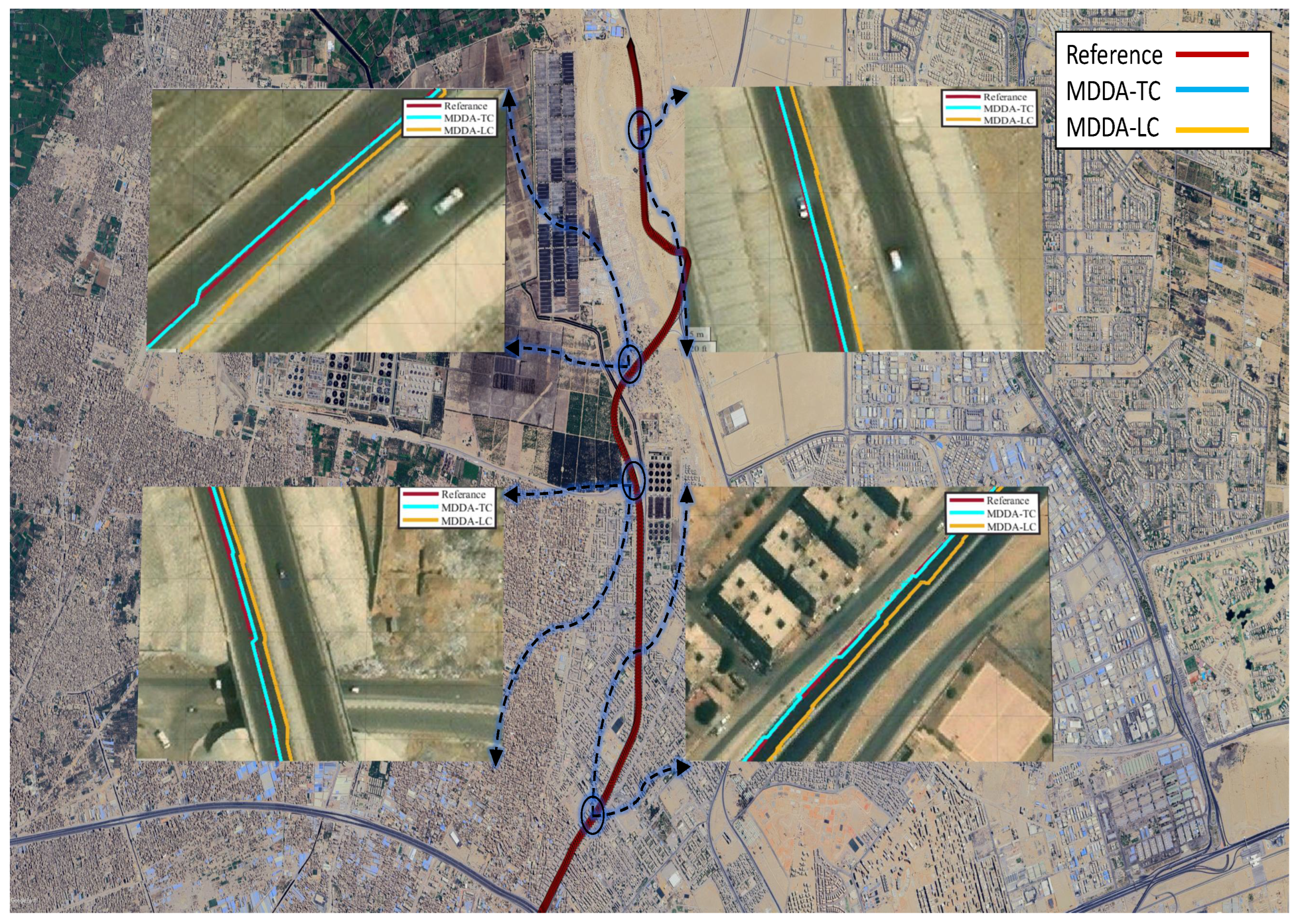
5.3. MDDA with TC Integration Scenario
6. Conclusions
Author Contributions
Funding
Institutional Review Board Statement
Informed Consent Statement
Data Availability Statement
Conflicts of Interest
References
- Li, Y.; Zhuang, Y.; Hu, X.; Gao, Z.; Hu, J.; Chen, L.; He, Z.; Pei, L.; Chen, K.; Wang, M.; et al. Toward Location-Enabled IoT (LE-IoT): IoT Positioning Techniques, Error Sources, and Error Mitigation. IEEE Internet Things J. 2021, 8, 4035–4062. [Google Scholar] [CrossRef]
- Chiang, K.W.; Huang, C.H.; Chang, H.W.; Lin, C.X.; Tsai, M.L.; Zeng, J.C.; Hung, M.C. Semantic proximity update of GNSS/INS/VINS for Seamless Vehicular Navigation using Smartphone sensors. IEEE Internet Things J. 2023, 10, 15736–15748. [Google Scholar] [CrossRef]
- Noureldin, A.; Karamat, T.B.; Georgy, J. Fundamentals of Inertial Navigation, Satellite-Based Positioning and Their Integration; Springer Science: Berlin/Heidelberg, Germany, 2012. [Google Scholar]
- Li, Y.; He, Z.; Gao, Z.; Zhuang, Y.; Shi, C.; El-Sheimy, N. Toward Robust Crowdsourcing-Based Localization: A Fingerprinting Accuracy Indicator Enhanced Wireless/Magnetic/Inertial Integration Approach. IEEE Internet Things J. 2019, 6, 3585–3600. [Google Scholar] [CrossRef]
- Abosekeen, A.; Iqbal, U.; Noureldin, A. Improved Navigation Through GNSS Outages: Fusing Automotive Radar and OBD-II Speed Measurements with Fuzzy Logic. GPS World 2021, 32, 36–41. [Google Scholar]
- Lin, J.; Zheng, C.; Xu, W.; Zhang, F. A Robust, Real-Time, LiDAR-Inertial-Visual Tightly-Coupled State Estimator and Mapping. IEEE Robot. Autom. Lett. 2021, 6, 7469–7476. [Google Scholar] [CrossRef]
- Li, S.; Wang, S.; Zhou, Y.; Shen, Z.; Li, X. Tightly Coupled Integration of GNSS, INS, and LiDAR for Vehicle Navigation in Urban Environments. IEEE Internet Things J. 2022, 9, 24721–24735. [Google Scholar] [CrossRef]
- Biancalana, C.; Gasparetti, F.; Micarelli, A.; Sansonetti, G. An Approach to Social Recommendation for Context-Aware Mobile Services. ACM Trans. Intell. Syst. Technol. 2013, 4, 1–31. [Google Scholar] [CrossRef]
- Mahdi, A.E.; Azouz, A.; Abdalla, A.E.; Abosekeen, A. A Machine Learning Approach for an Improved Inertial Navigation System Solution. Sensors 2022, 22, 1687. [Google Scholar] [CrossRef]
- Alam, N.; Balaei, A.T.; Dempster, A.G. Relative positioning enhancement in VANETs: A tight integration approach. IEEE Trans. Intell. Transp. Syst. 2012, 14, 47–55. [Google Scholar] [CrossRef]
- El-Khalea, M.F.; Hendy, H.M.; Kamel, A.M.; Arafa, I.I. Loosely Coupled GNSS/INS for Android Platforms. In Proceedings of the 2022 13th International Conference on Electrical Engineering (ICEENG), Cairo, Egypt, 29–31 March 2022; pp. 37–41. [Google Scholar] [CrossRef]
- Yi, D.; Yang, S.; Bisnath, S. Native Smartphone Single-and Dual-Frequency GNSS-PPP/IMU Solution in Real-World Driving Scenarios. Remote Sens. 2022, 14, 3286. [Google Scholar] [CrossRef]
- Iqbal, U.; Abosekeen, A.; Elsheikh, M.; Noureldin, A.; Korenberg, M.J. A Review of Sensor System Schemes for Integrated Navigation. In Proceedings of the 2022 5th International Conference on Communications, Signal Processing, and their Applications (ICCSPA), Cairo, Egypt, 27–29 December 2022; pp. 1–5. [Google Scholar] [CrossRef]
- Li, X.; Wang, H.; Li, S.; Feng, S.; Wang, X.; Liao, J. GIL: A tightly coupled GNSS PPP/INS/LiDAR method for precise vehicle navigation. Satell. Navig. 2021, 2, 26. [Google Scholar] [CrossRef]
- Ibrahim, A.; Abosekeen, A.; Azouz, A.; Noureldin, A. Enhanced Autonomous Vehicle Positioning Using a Loosely Coupled INS/GNSS-Based Invariant-EKF Integration. Sensors 2023, 23, 6097. [Google Scholar] [CrossRef] [PubMed]
- European Union Agency for the Space Programme. Using GNSS Raw Measurements on Android Devices. White Paper, 28 January 2018. Available online: https://www.gsa.europa.eu/system/files/reports/gnss_raw_measurement_web_0.pdf (accessed on 3 May 2022).
- Radicati Group. Mobile Statistics Report, 2021–2025—Executive Summary 2021. Available online: https://www.radicati.com/wp/wp-content/uploads/2021/Mobile_Statistics_Report,_2021-2025_Executive_Summary.pdf (accessed on 23 April 2025).
- Suzuki, T. Precise Position Estimation Using Smartphone Raw GNSS Data Based on Two-Step Optimization. Sensors 2023, 23, 1205. [Google Scholar] [CrossRef] [PubMed]
- ElKhalea, M.F.; Hendy, H.M.; Kamel, A.M.; Arafa, I.I.; Abosekeen, A. Smartphone Positioning Enhancement Using Several GNSS Satellite Selection Techniques. In Proceedings of the 2022 5th International Conference on Communications, Signal Processing, and their Applications (ICCSPA), Cairo, Egypt, 27–29 December 2022; pp. 1–6. [Google Scholar] [CrossRef]
- Zhou, J.; Knedlik, S.; Loffeld, O. INS/GPS tightly-coupled integration using adaptive unscented particle filter. J. Navig. 2010, 63, 491–511. [Google Scholar] [CrossRef]
- Lu, Y.; Ji, S.; Chen, W.; Wang, Z. Assessing the performance of raw measurement from different types of smartphones. In Proceedings of the 31st International Technical Meeting of the Satellite Division of the Institute of Navigation (ION GNSS+ 2018), Miami, FL, USA, 24–28 September 2018; pp. 304–322. [Google Scholar] [CrossRef]
- Li, L.; Elhajj, M.; Feng, Y.; Ochieng, W.Y. Machine learning based GNSS signal classification and weighting scheme design in the built environment: A comparative experiment. Satell. Navig. 2023, 4, 21. [Google Scholar] [CrossRef]
- Gogoi, N.; Minetto, A.; Linty, N.; Dovis, F. A controlled-environment quality assessment of android GNSS raw measurements. Electronics 2018, 8, 5. [Google Scholar] [CrossRef]
- Gomes, A.; Krueger, C.P. Evaluation of the positional quality through the post-processing of raw GNSS data from a smartphone via different satellite positioning methods. Boletim Ciências Geodésicas 2020, 26, e2020020. [Google Scholar] [CrossRef]
- Chen, R.; Zhao, L. Multi-level autonomous integrity monitoring method for multi-source PNT resilient fusion navigation. Satell. Navig. 2023, 4, 21. [Google Scholar] [CrossRef]
- Alghisi, M.; Biagi, L. Positioning with GNSS and 5G: Analysis of Geometric Accuracy in Urban Scenarios. Sensors 2023, 23, 2181. [Google Scholar] [CrossRef]
- Niu, X.; Zhang, Q.; Li, Y.; Cheng, Y.; Shi, C. Using inertial sensors of iPhone 4 for car navigation. In Proceedings of the 2012 IEEE/ION Position, Location and Navigation Symposium, Myrtle Beach, SC, USA, 23–26 April 2012; pp. 555–561. [Google Scholar] [CrossRef]
- Sheta, A.; Mohsen, A.; Sheta, B.; Hassan, M. Improved localization for Android smartphones based on integration of raw GNSS measurements and IMU sensors. In Proceedings of the 2018 International Conference on Computer and Applications (ICCA), Beirut, Lebanon, 25–26 August 2018; pp. 297–302. [Google Scholar] [CrossRef]
- Robustelli, U.; Baiocchi, V.; Pugliano, G. Assessment of dual frequency GNSS observations from a Xiaomi Mi 8 Android smartphone and positioning performance analysis. Electronics 2019, 8, 91. [Google Scholar] [CrossRef]
- Paziewski, J.; Fortunato, M.; Mazzoni, A.; Odolinski, R. An analysis of multi-GNSS observations tracked by recent Android smartphones and smartphone-only relative positioning results. Measurement 2021, 175, 109162. [Google Scholar] [CrossRef]
- Kuutti, S.; Fallah, S.; Katsaros, K.; Dianati, M.; Mccullough, F.; Mouzakitis, A. A survey of the state-of-the-art localization techniques and their potentials for autonomous vehicle applications. IEEE Internet Things J. 2018, 5, 829–846. [Google Scholar] [CrossRef]
- Lee, D.K.; Taylor, T.; Akos, D.M.; Yun, J.; Jo, Y.; Park, B. GNSS Fault Detection and Mitigation using Android IMU. In Proceedings of the 35th International Technical Meeting of the Satellite Division of The Institute of Navigation (ION GNSS+ 2022), Denver, CO, USA, 19–23 September 2022; pp. 1676–1686. [Google Scholar] [CrossRef]
- Chai, D.; Song, S.; Wang, K.; Bi, J.; Zhang, Y.; Ning, Y.; Yan, R. Optimization Model-Based Robust Method and Performance Evaluation of GNSS/INS Integrated Navigation for Urban Scenes. Electronics 2025, 14, 660. [Google Scholar] [CrossRef]
- Prochniewicz, D.; Kudrys, J.; Maciuk, K. Noises in Double-Differenced GNSS Observations. Energies 2022, 15, 1668. [Google Scholar] [CrossRef]
- Angrisano, A.; Del Pizzo, S.; Gaglione, S.; Troisi, S.; Vultaggio, M. Using local redundancy to improve GNSS absolute positioning in harsh scenario. Acta Imeko 2018, 7, 16–23. [Google Scholar] [CrossRef]
- Hartinger, H.; Brunner, F.K. Variances of GPS phase observations: The SIGMA model. GPS Solut. 1999, 2, 35–43. [Google Scholar] [CrossRef]
- Angrisano, A.; Del Pizzo, S.; Gaglione, S.; Troisi, S.; Vultaggio, M. Enhanced pseudorange weighting scheme using local redundancy. In Proceedings of the IMEKO International Conference on Metrology for The Sea Naples, Naples, Italy, 11–13 October 2017. [Google Scholar]
- Shinghal, G.; Bisnath, S. Conditioning and PPP processing of smartphone GNSS measurements in realistic environments. Satell. Navig. 2021, 2, 10. [Google Scholar] [CrossRef]
- Banville, S.; Lachapelle, G.; Ghoddousi-Fard, R.; Gratton, P. Automated processing of low-cost GNSS receiver data. In Proceedings of the 32nd International Technical Meeting of the Satellite Division of The Institute of Navigation (ION GNSS+ 2019), Miami, FL, USA, 16–20 September 2019; pp. 3636–3652. [Google Scholar]
- Medina, D.; Gibson, K.; Ziebold, R.; Closas, P. Determination of pseudorange error models and multipath characterization under signal-degraded scenarios. In Proceedings of the 31st International Technical Meeting of the Satellite Division of the Institute of Navigation, ION GNSS+ 2018, Miami, FL, USA, 24–28 September 2018. [Google Scholar]
- Lyu, Z.; Gao, Y. An SVM based weight scheme for improving kinematic GNSS positioning accuracy with low-cost GNSS receiver in urban environments. Sensors 2020, 20, 7265. [Google Scholar] [CrossRef]
- Manandhar, S.; Meng, Y.S. Analysis on the effect of different elevation cut-off angles on GPS time transfer. Meas. Sens. 2021, 18, 100196. [Google Scholar] [CrossRef]
- Walter, T.; Blanch, J.; Kropp, V. Satellite selection for multi-constellation SBAS. In Proceedings of the 29th International Technical Meeting of the Satellite Division of the Institute of Navigation (ION GNSS+ 2016), Portland, OR, USA, 12–16 September 2016; pp. 1350–1359. [Google Scholar]
- Deng, Z.l.; Dong, H.; Zhan, Z.w.; Wang, G.y.; Yin, L.; Xi, Y. Improved satellite selection algorithm based on carrier-to-noise ratio and geometric dilution of precision. In China Satellite Navigation Conference (CSNC) 2013 Proceedings: BeiDou/GNSS Navigation Applications Test & Assessment Technology User Terminal Technology; Springer: Berlin/Heidelberg, Germany, 2013; pp. 575–583. [Google Scholar]
- He, G.; Song, M.; He, X.; Hu, Y. GPS signal acquisition based on compressive sensing and modified greedy acquisition algorithm. IEEE Access 2019, 7, 40445–40453. [Google Scholar] [CrossRef]
- Chi, C.; Zhan, X.; Wu, T.; Zhang, X. Ultra-rapid direct satellite selection algorithm for multi-GNSS. In International Conference on Aerospace System Science and Engineering 2019; Springer: Singapore, 2020; pp. 11–25. [Google Scholar]
- Odenwald, S. A Guide to Smartphone Sensors Experimeter’ s Guide to Smartphone Sensors; National Aeronautics and Space Administration: Washington, DC, USA, 2019. [Google Scholar]
- Bosch Sensortec. BMI160 Small, Low Power Inertial Measurement Unit. 2015. Available online: https://www.bosch-sensortec.com (accessed on 10 October 2023).
- Groves, P. Principles of GNSS, Inertial, and Multisensor Integrated Navigation Systems, 2nd ed.; GNSS/GPS, Artech House: London, UK, 2013. [Google Scholar]
- Kourabbaslou, S.S.; Zhang, A.; Atia, M.M. A Novel Design Framework for Tightly Coupled IMU/GNSS Sensor Fusion Using Inverse-Kinematics, Symbolic Engines, and Genetic Algorithms. IEEE Sens. J. 2019, 19, 11424–11436. [Google Scholar] [CrossRef]
- Diebel, J. Representing attitude: Euler angles, unit quaternions, and rotation vectors. Matrix 2006, 58, 1–35. [Google Scholar]
- Elsabbagh, M.S.; Hassaballa, A.H.; Kamel, A.M.; Elhalwagy, Y.Z. Precise Orientation Estimation Based on Nonlinear Modeling and Quaternion Transformations for Low Cost Navigation Systems. In Proceedings of the 2021 3rd Novel Intelligent and Leading Emerging Sciences Conference (NILES), Giza, Egypt, 23–25 October 2021; pp. 147–154. [Google Scholar] [CrossRef]
- Atia, M. Design and simulation of sensor fusion using symbolic engines. Math. Comput. Model. Dyn. Syst. 2019, 25, 40–62. [Google Scholar] [CrossRef]
- Grewal, M.S.; Andrews, A.P.; Bartone, C.G. Global Navigation Satellite Systems, Inertial Navigation, and Integration; John Wiley & Sons: Hoboken, NJ, USA, 2020. [Google Scholar]
- Diggelen, F.V.; Want, R.; Wang, W. How to Achieve 1-Meter Accuracy in Android. Available online: https://www.gpsworld.com/how-to-achieve-1-meter-accuracy-in-android/ (accessed on 15 October 2023).
- Google Developers. Fused Location Provider. Available online: https://developers.google.com/location-context/fused-location-provider (accessed on 15 October 2023).
- Abosekeen, A.; Iqbal, U.; Noureldin, A.; Korenberg, M.J. A novel multi-level integrated navigation system for challenging GNSS environments. IEEE Trans. Intell. Transp. Syst. 2020, 22, 4838–4852. [Google Scholar] [CrossRef]


| Gyroscope | Accelerometer | |
|---|---|---|
| Max measurement range | ||
| Bias error | ||
| Output noise | ||
| Resolution |
| Method | ||
|---|---|---|
| All Visible Satellites | ||
| All Satellites | 4.58 | 11.89 |
| MDDA-Based | 3.96 | 6.78 |
| Selected Satellites According to Max. Number of Rx Channels (10 Satellites) | ||
| 10 EL-Based | 5.67 | 7.59 |
| 10 CNR-Based | 5.43 | 7.40 |
| 10 MDDA-Based | 4.96 | 7.17 |
| Method | East | North | Down | 2D Position | 3D Position |
|---|---|---|---|---|---|
| All Visible Satellites | |||||
| All Satellites | 3.17 | 1.98 | 2.12 | 3.74 | 4.30 |
| MDDA-LC-Based | 2.86 | 1.89 | 1.9 | 3.43 | 3.95 |
| Selected Satellites According to Max. Number of Rx Channels (10 Satellites) | |||||
| 10 EL-LC-Based | 3.76 | 2.52 | 2.41 | 4.53 | 5.13 |
| 10 CNR-LC-Based | 3.19 | 2.17 | 2.21 | 3.86 | 4.45 |
| 10 MDDA-LC-Based | 3.18 | 1.99 | 2.06 | 3.75 | 4.28 |
| Method | East | North | Down | 2D Position | 3D Position |
|---|---|---|---|---|---|
| All Visible Satellites | |||||
| All Satellites | 0.66 | 0.54 | 0.82 | 0.86 | 1.19 |
| MDDA-TC-Based | 0.64 | 0.54 | 0.82 | 0.84 | 1.17 |
| Selected Satellites According to Max. Number of Rx Channels (10 Satellites) | |||||
| 10 EL-TC-Based | 0.64 | 0.73 | 1.05 | 0.97 | 1.43 |
| 10 CNR-TC-Based | 0.63 | 0.72 | 0.94 | 0.95 | 1.34 |
| 10 MDDA-TC-Based | 0.58 | 0.69 | 0.92 | 0.91 | 1.29 |
| EL-Based | CNR-Based | MDDA-Based | |
|---|---|---|---|
| Geometric Dilution of Precision (GDOP) | 1.90 | 1.73 | 1.67 |
| Horizontal Dilution of Precision (HDOP) | 1.54 | 1.35 | 1.28 |
| Position Dilution of Precision (PDOP) | 1.70 | 1.56 | 1.50 |
Disclaimer/Publisher’s Note: The statements, opinions and data contained in all publications are solely those of the individual author(s) and contributor(s) and not of MDPI and/or the editor(s). MDPI and/or the editor(s) disclaim responsibility for any injury to people or property resulting from any ideas, methods, instructions or products referred to in the content. |
© 2025 by the authors. Licensee MDPI, Basel, Switzerland. This article is an open access article distributed under the terms and conditions of the Creative Commons Attribution (CC BY) license (https://creativecommons.org/licenses/by/4.0/).
Share and Cite
Elkhalea, M.F.; Hendy, H.; Kamel, A.; Abosekeen, A.; Noureldin, A. Centralized Measurement Level Fusion of GNSS and Inertial Sensors for Robust Positioning and Navigation. Sensors 2025, 25, 2804. https://doi.org/10.3390/s25092804
Elkhalea MF, Hendy H, Kamel A, Abosekeen A, Noureldin A. Centralized Measurement Level Fusion of GNSS and Inertial Sensors for Robust Positioning and Navigation. Sensors. 2025; 25(9):2804. https://doi.org/10.3390/s25092804
Chicago/Turabian StyleElkhalea, Mohamed F., Hossam Hendy, Ahmed Kamel, Ashraf Abosekeen, and Aboelmagd Noureldin. 2025. "Centralized Measurement Level Fusion of GNSS and Inertial Sensors for Robust Positioning and Navigation" Sensors 25, no. 9: 2804. https://doi.org/10.3390/s25092804
APA StyleElkhalea, M. F., Hendy, H., Kamel, A., Abosekeen, A., & Noureldin, A. (2025). Centralized Measurement Level Fusion of GNSS and Inertial Sensors for Robust Positioning and Navigation. Sensors, 25(9), 2804. https://doi.org/10.3390/s25092804