
Vehicle Recognition and Driving Information Detection with UAV Video Based on Improved YOLOv5-DeepSORT Algorithm


Abstract
1. Introduction
2. Basic Principle of YOLO Algorithm
2.1. Training of YOLO Algorithm
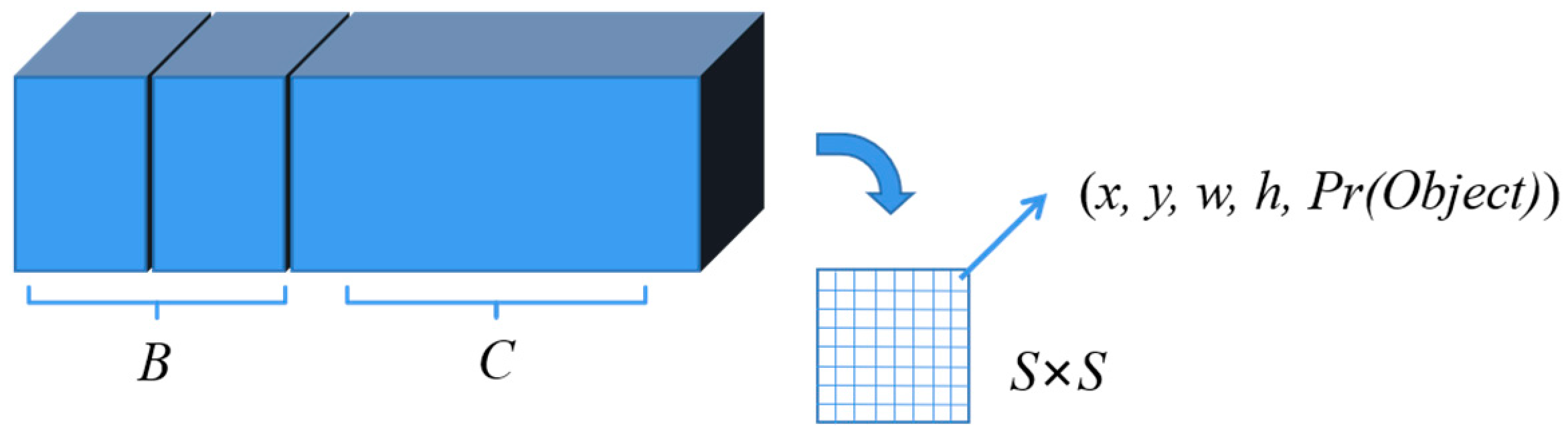
2.2. Detection Principle of YOLO Algorithm
3. Labeling and Training of Vehicles with UAV Video
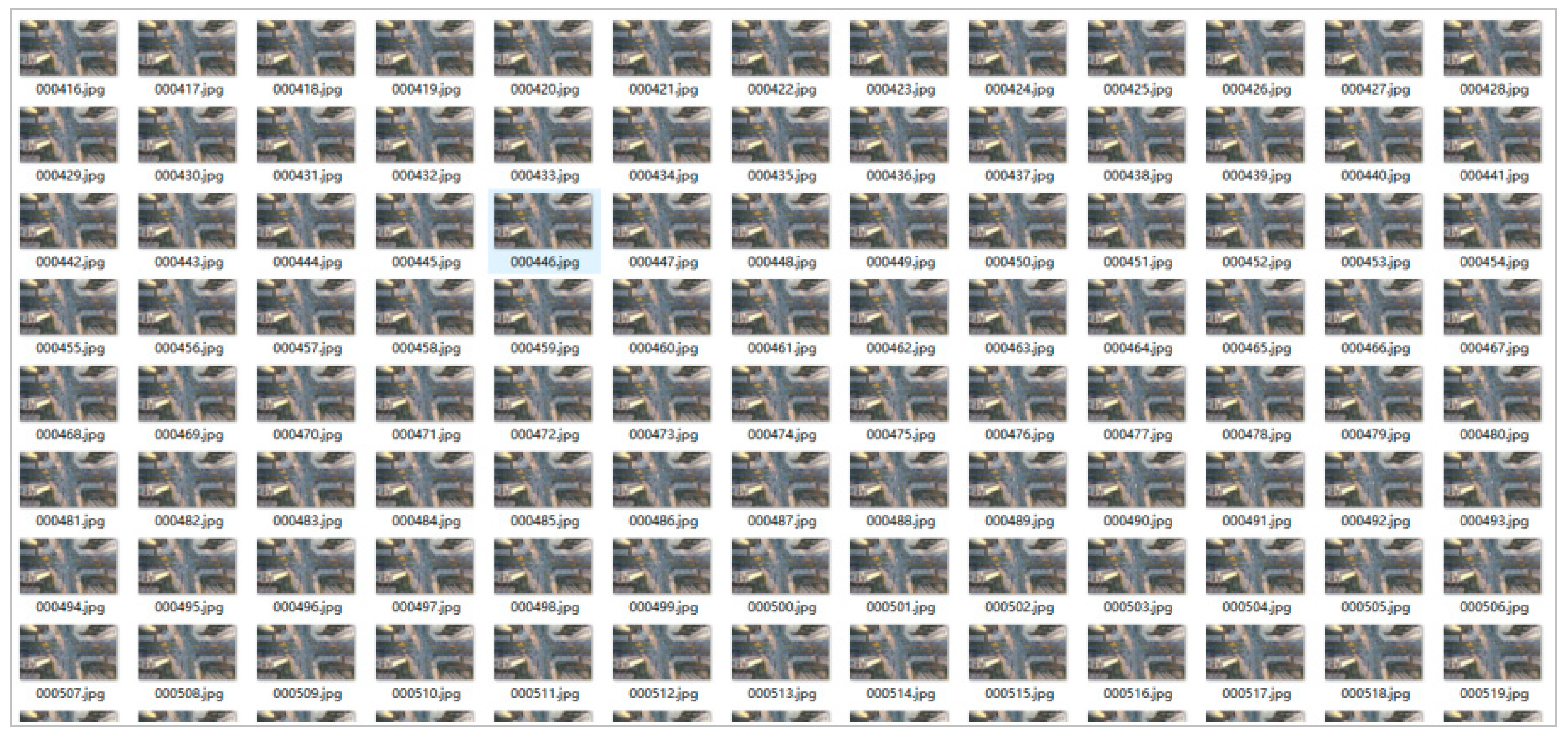
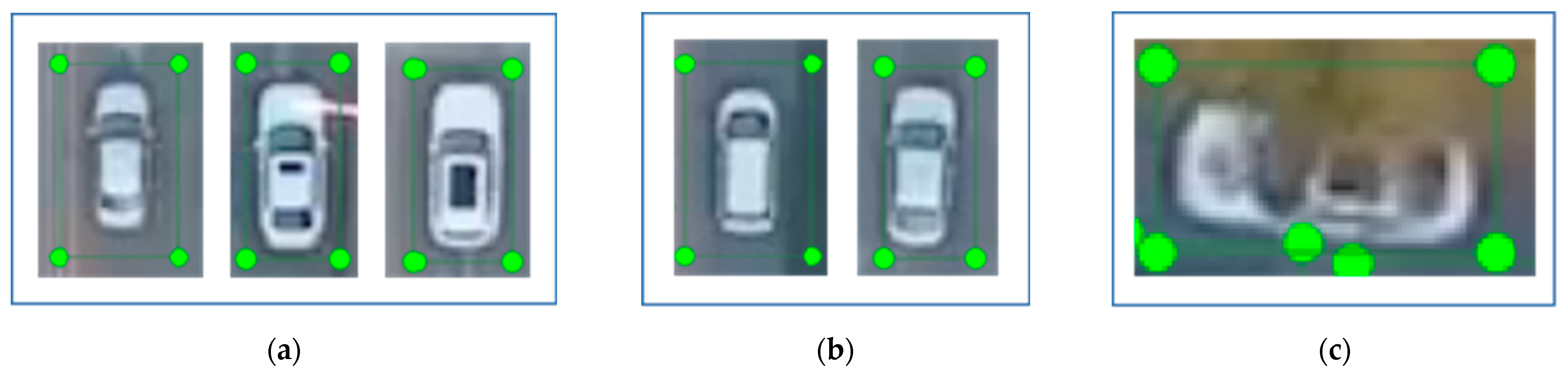
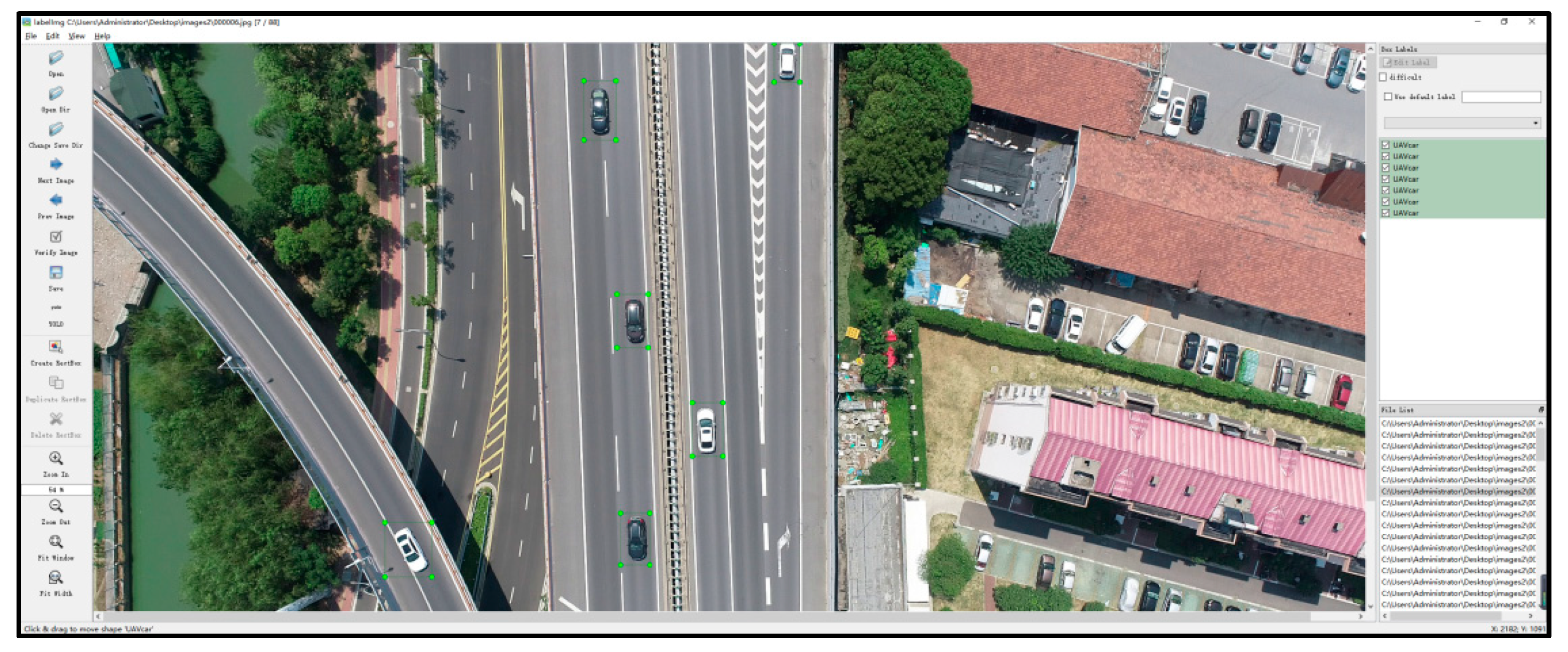
3.1. Labeling of Vehicles with UAV Video
| Code 1. UAV video key frame extraction and storage | |
| 1 | import cv2 |
| 2 | import os |
| 3 | # location of the video to be extracted |
| 4 | video_path=r”./UAVvid1.mp4” |
| 5 | # location of the image to be saved |
| 6 | img_path=r’./Images’ |
| 7 | vidcap = cv2.VideoCapture(video_path) |
| 8 | (cap,frame)= vidcap.read() |
| 9 | while cap: |
| 10 | cv2.imwrite(os.path.join(img_path,’%.6d.jpg’%count),frame) |
| 11 | print(‘%.6d.jpg’%count) |
| 12 | count += 1 |
| … | |
| Code 2. Dataset partitioning and label configuration | |
| 1 | train: ./data/yolo_UAV/images/train |
| 2 | val: ./data/yolo_UAV/images/val |
3.2. Results of YOLO Training
3.3. Field Test
4. Vehicle Information Extraction Based on Improved YOLOv5-DeepSORT
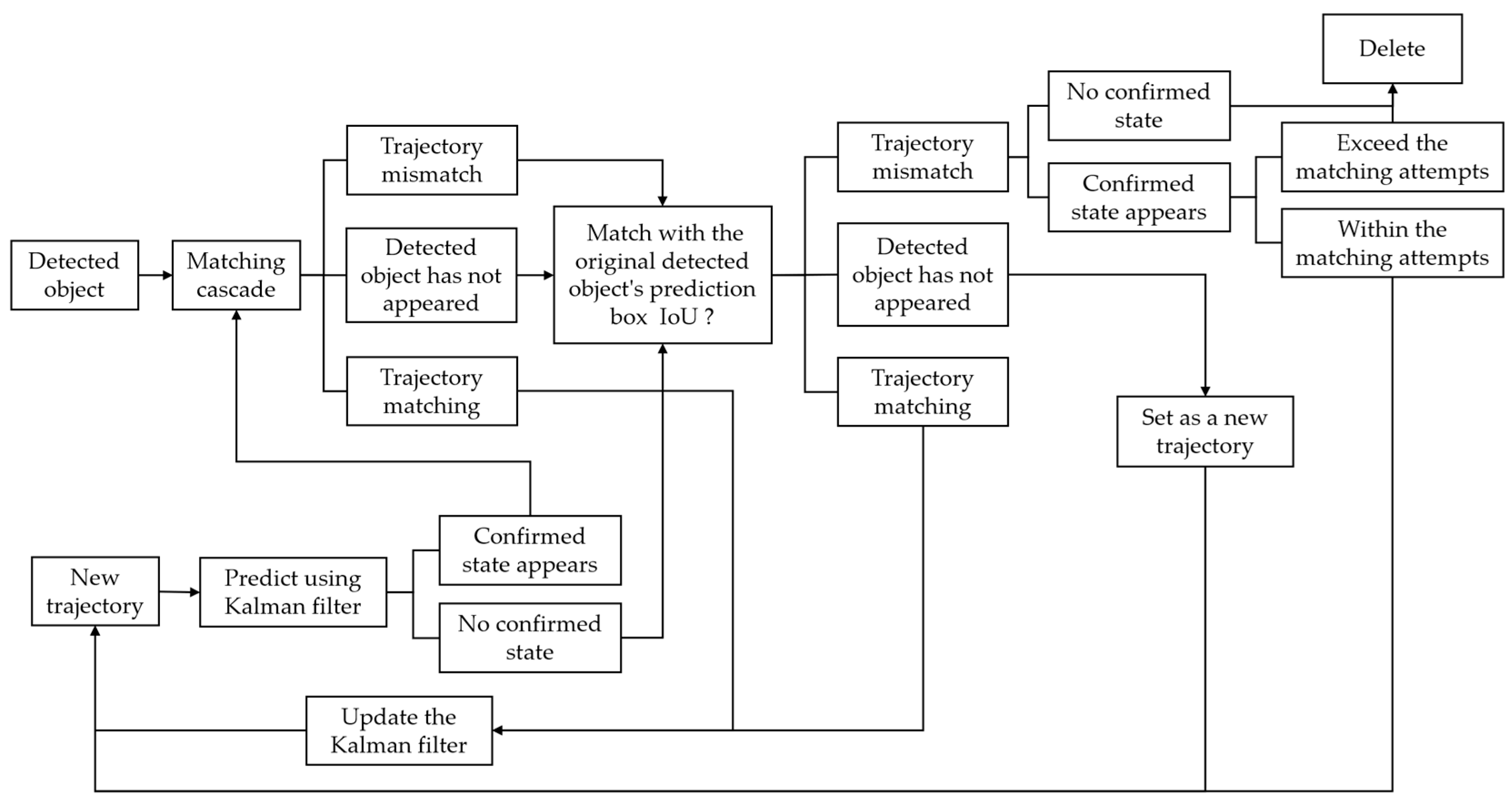
4.1. Improvement of DeepSORT Algorithm
| Code 3. YOLOv5-compatible target tracking module | |
| … | |
| 1 | self.yolo_bbox = [0, 0, 0, 0] |
| … | |
| 2 | def get_yolo_pred(self): |
| 3 | return self.yolo_bbox |
| … | |
| 4 | def update(self, kf, detection, class_id): |
| 5 | self.yolo_bbox = detection |
| … | |
| Code 4. Main program tracking logic update | |
| … | |
| 1 | def update(self, bbox_xywh, confidences, classes, ori_img, use_yolo_preds=True): |
| 2 | self.height, self.width = ori_img.shape[:2] |
| … | |
| 3 | for track in self.tracker.tracks: |
| 4 | if not track.is_confirmed() or track.time_since_update > 1: |
| 5 | continue |
| 6 | if use_yolo_preds: |
| 7 | det = track.get_yolo_pred() |
| 8 | x1, y1, x2, y2 = self._tlwh_to_xyxy(det.tlwh) |
| 9 | else: |
| 10 | box = track.to_tlwh() |
| 11 | x1, y1, x2, y2 = self._tlwh_to_xyxy(box) |
| 12 | track_id = track.track_id |
| 13 | class_id = track.class_id |
| 14 | outputs.append(np.array([x1, y1, x2, y2, track_id, class_id], dtype=np.int)) |
| … | |
4.2. Vehicle Coordinate Transformation
4.3. Vehicle Trajectory Extraction
4.3.1. Vehicle Information Acquisition
| Code 5. Vehicle trajectory center coordinate extraction | |
| 1 | if len(outputs) > 0: |
| 2 | for j, (output, conf) in enumerate(zip(outputs, confs)): |
| 3 | bboxes = output[0:4] # extract coordinate information |
| 4 | id = output[4] # extract vehicle ID information |
| 5 | cls = output[5] # extract vehicle class information |
| … | |
| 6 | if save_txt: |
| 7 | x_center = output[0] / 2 + output[2] / 2 # calculate the x-coordinate of the bbox center |
| 8 | y_center = output[0] / 2 + output[2] / 2 # calculate the y-coordinate of the bbox center |
| 9 | with open(txt_path, ’a’) as f: |
| 10 | f.write((‘%g ‘ * 10 + ‘\n’) % (frame_idx + 1, id, x_center, y_center,)) # write (frame number, ID, bbox center x, bbox center y) |
4.3.2. Vehicle Trajectory Drawing
| Code 6. Real-time vehicle trajectory visualization | |
| 1 | if len(outputs) > 0: |
| 2 | for j, (output, conf) in enumerate(zip(outputs, confs)): |
| 3 | bbox_xyxy = output[0:4] # extract coordinate information |
| 4 | id = output[4] # extract vehicle ID information |
| 5 | x_center = bbox_xyxy[0] /2 + bbox_xyxy[2] / 2 # calculate the x-coordinate of the bbox center |
| 6 | y_center = bbox_xyxy[1] /2 + bbox_xyxy[3] / 2 # calculate the y-coordinate of the bbox center |
| 7 | center = [x_center, y_center] |
| 8 | dict_box.setdefault(id, []).append(center) # call Python dictionary |
| 9 | if frame_idx > 2: # skip first 2 frames (DeepSORT can’t draw); start from frame 3 |
| 10 | for key, value in dict_box.items(): |
| 11 | for a in range(len(value) − 1): |
| 12 | color = COLORS_10[key % len(COLORS_10)] # set trajectory color |
| 13 | index_start = a |
| 14 | index_end = index_start + 1 |
| 15 | cv2.line(im0, tuple(map(int, value[index_start])), tuple(map(int, value[index_end])), color, thickness=2, lineType=8) # draw trajectory line |
4.3.3. Vehicle Trajectory Smoothing
5. Conclusions
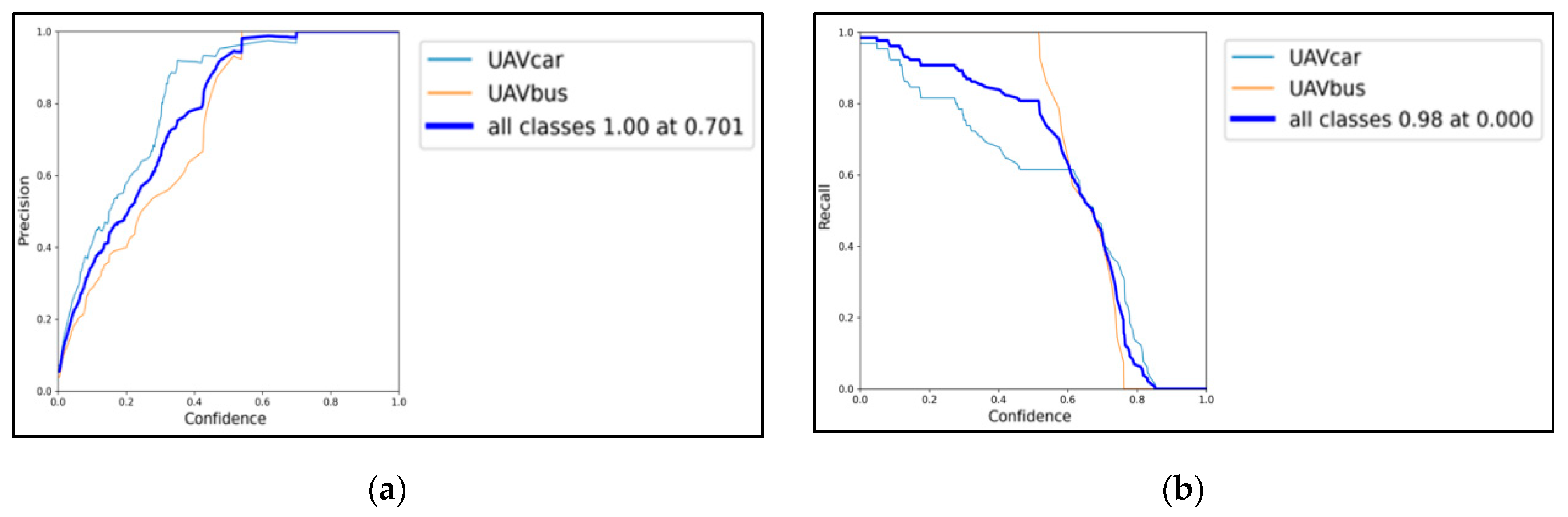
- (1)
- As the confidence of learning increases, there is a very significant increase in P, and eventually, a 100% precision rate is achieved for all categories of objects at the confidence of 0.701. There is a significant decrease in the R, and R eventually decreases to 0 at the confidence of 0.98 for all categories of objects. For the dominant small cars, it also decreases to 0 at the confidence of more than 0.9, indicating that the learned YOLO has a high recognition success for small cars. For large vehicles, the recall rate decreases to 0 at the confidence of more than 0.75, which is caused by too few samples and inconspicuous aerial photo features of large vehicles, but YOLO still has a high recognition accuracy.
- (2)
- As R increases, the number of objects of a certain category that are predicted increases; i.e., those with a lower probability are gradually predicted, which shows that the YOLO model is fairly effective in recognizing vehicles from aerial videos. The model overall reaches the maximum F1 value of 0.86 at the confidence of 0.516, balancing the PR relationship very well. The PR plot and F1 value together reflect that the training has quite stable results and high accuracy.
- (3)
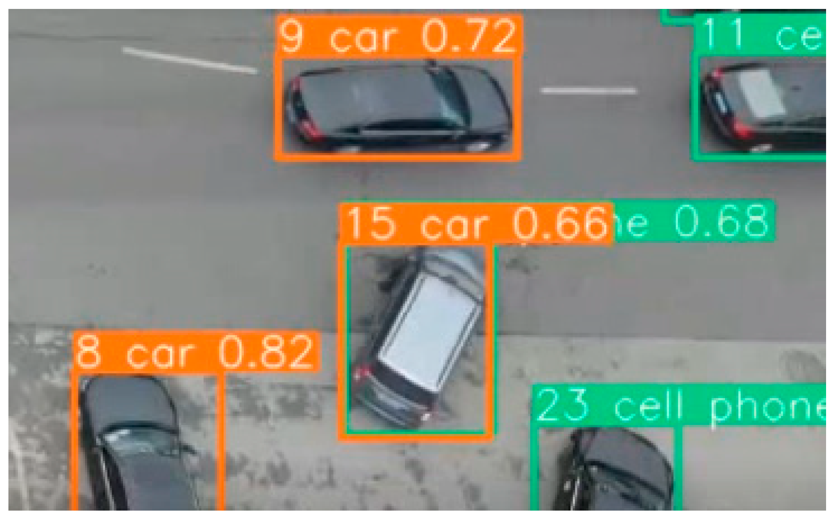
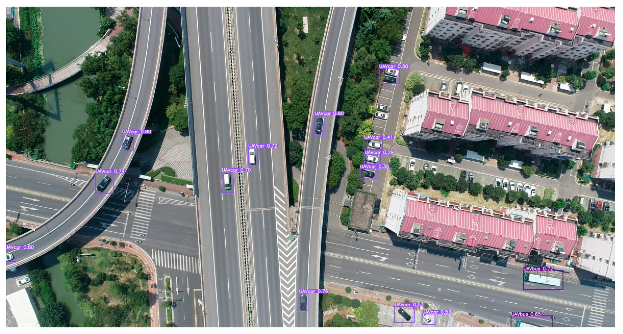
- The loss in both the training and validation sets decreases significantly with the increase of training epoch, and the loss function reaches a stable and low level after 70 training epochs. The mAP@0.5 and mAP@[0.5:0.95] plots also reflect stability at over 70 epochs, exceeding 90% and 40%, respectively, and the extracted video frames also show good recognition results. The actual detection results show that the YOLOv5 recognition algorithm reprogrammed in this study is very accurate and can be well applied in vehicle detection.
- (4)
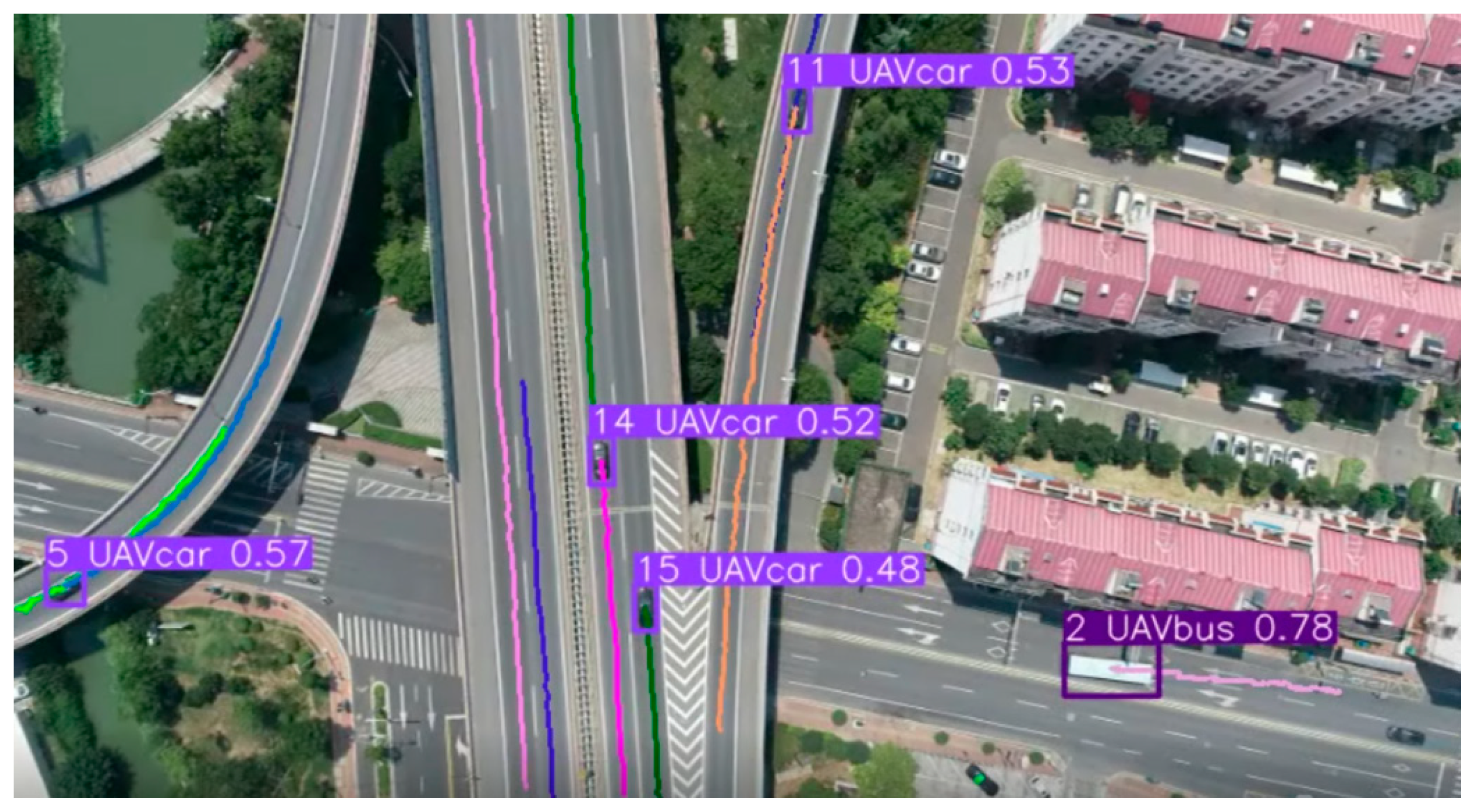
- The trained YOLOv5 target detection algorithm replaces the original Faster R-CNN detector in DeepSORT, improving the detection accuracy and efficiency; the coordinate transformation calculations are performed between the UAV video of DJI Mavic 2 Pro and the actual road, to convert UAV video pixel coordinates to real-world spatial scales. Vehicle trajectory, speed and other elements are extracted, and the vehicle trajectory lines are smoothed to construct a more realistic model, avoiding the impact of “jagged” trajectories on the maneuverability of the driver model.
Author Contributions
Funding
Institutional Review Board Statement
Informed Consent Statement
Data Availability Statement
Conflicts of Interest
References
- Murphy, D.W.; Bott, J.P. On the Lookout: The Air Mobile Ground Security and Surveillance System (AMGSS) Has Arrived. In Proceedings of the 10th Annual ADPA Security Technology Symposium, Washington, DC, USA, 20–23 June 1995. [Google Scholar]
- Montanino, M.; Punzo, V. Making NGSIM Data Usable for Studies on Traffic Flow Theory: Multistep Method for Vehicle Trajectory Reconstruction. J. Transp. Res. Board 2013, 2390, 99–111. [Google Scholar] [CrossRef]
- Kumar, S.; Paefgen, J.; Wilhelm, E.; Sarma, S.E. Integrating On-board Diagnostics Speed Data with Sparse GPS Measurements for Vehicle Trajectory Estimation. In Proceedings of the SICE Conference, Nagoya, Japan, 14–17 September 2013; IEEE: Piscataway, NJ, USA, 2013. [Google Scholar]
- Wright, T.J.; Vitale, T.; Boot, W.R.; Charness, N. The Impact of Red Light Running Camera Flashes on Younger and Older Drivers’ Attention and Oculomotor Control. Psychol. Aging 2015, 30, 755–766. [Google Scholar] [CrossRef]
- Leyva-Mayorga, I.; Martinez-Gost, M.; Moretti, M.; Pérez-Neira, A.; Vázquez, M.Á.; Popovski, P.; Soret, B. Satellite Edge Computing for Real-Time and Very-High Resolution Earth Observation. IEEE Trans. Commun. 2023, 71, 6180–6194. [Google Scholar] [CrossRef]
- Zhao, X.; Pu, F.; Wang, H.; Chen, H.; Xu, Z. Detection, Tracking, and Geolocation of Moving Vehicle from UAV Using Monocular Camera. IEEE Access 2019, 7, 101160–101170. [Google Scholar] [CrossRef]
- Sun, L.; Zhang, J.; Yang, Z.; Fan, B. A Motion-Aware Siamese Framework for Unmanned Aerial Vehicle Tracking. Drones 2023, 7, 153. [Google Scholar] [CrossRef]
- Avola, D.; Cinque, L.; Di Mambro, A.; Diko, A.; Fagioli, A.; Foresti, G.L.; Marini, M.R.; Mecca, A.; Pannone, D. Low-Altitude Aerial Video Surveillance via One-Class SVM Anomaly Detection from Textural Features in UAV Images. Information 2022, 13, 2. [Google Scholar] [CrossRef]
- Li, J.; Chen, S.; Zhang, F.; Li, E.; Yang, T.; Lu, Z. An Adaptive Framework for Multi-Vehicle Ground Speed Estimation in Airborne Videos. Remote Sens. 2019, 11, 1241. [Google Scholar] [CrossRef]
- Salvo, G.; Caruso, L.; Scordo, A. Urban Traffic Analysis through an UAV. Procedia Soc. Behav. Sci. 2014, 111, 1083–1091. [Google Scholar] [CrossRef]
- Cao, X.; Wang, Z.; Zheng, B.; Tan, Y. Improved UAV-to-Ground Multi-Target Tracking Algorithm Based on StrongSORT. Sensors 2023, 23, 9239. [Google Scholar] [CrossRef]
- Shan, D.; Lei, T.; Yin, X.; Luo, Q.; Gong, L. Extracting Key Traffic Parameters from UAV Video with On-Board Vehicle Data Validation. Sensors 2021, 21, 5620. [Google Scholar] [CrossRef]
- Xiang, X.; Zhai, M.; Lv, N.; El Saddik, A. Vehicle Counting Based on Vehicle Detection and Tracking from Aerial Videos. Sensors 2018, 18, 2560. [Google Scholar] [CrossRef]
- Coifman, B.; McCord, M.; Mishalani, R.G.; Redmill, K. Surface Transportation Surveillance from Unmanned Aerial Vehicles. In Proceedings of the 83rd Annual Meeting of the Transportation Research Board, Washington, DC, USA, 11–15 January 2004. [Google Scholar]
- Coifman, B.; McCord, M.; Mishalani, R.G.; Iswalt, M.; Ji, Y. Roadway Traffic Monitoring from an Unmanned Aerial Vehicle. IEE Proc. Intell. Transp. Syst. 2006, 153, 11–20. [Google Scholar] [CrossRef]
- Agrawal, A.; Hickman, M. Automated Extraction of Queue Lengths from Airborne Imagery. In Proceedings of the IEEE International Conference on Intelligent Transportation Systems, Washington, DC, USA, 3–6 October 2004. [Google Scholar]
- Ruhe, M.; Kühne, R.; Ernst, I.; Zuev, S.; Hipp, E. Air Borne Systems and Data Fusion for Traffic Surveillance and Forecast for the Soccer World Cup. In Proceedings of the 86th Annual Meeting of the Transportation Research Board, Washington, DC, USA, 21–25 January 2007. [Google Scholar]
- Wang, Y. Research on Moving Vehicle Detection Based on UAV Video. Master’s Thesis, Beijing Jiaotong University, Beijing, China, 2017. [Google Scholar]
- Liu, H. Study on Multi-Object Detection and Tracking in Video Captured from Low-Altitude Platform. Ph.D. Thesis, Wuhan University, Wuhan, China, 2013. [Google Scholar]
- Terzopoulos, D.; Szeliski, R. Tracking with Kalman Snakes. In Active Vision; MIT Press: Cambridge, MA, USA, 1993; pp. 3–20. [Google Scholar]
- Isard, M.; Blake, A. Contour Tracking by Stochastic Propagation of Conditional Density. In Proceedings of the European Conference on Computer Vision (ECCV), Cambridge, UK, 14–18 April 1996; Springer: Berlin/Heidelberg, Germany, 1996; pp. 343–356. [Google Scholar]
- Rad, R.; Jamzad, M. Real-Time Classification and Tracking of Multiple Vehicles in Highways. Pattern Recognit. Lett. 2005, 26, 1597–1607. [Google Scholar] [CrossRef]
- Jones, R.; Ristic, B.; Redding, N.J.; Booth, D.M. Moving Target Indication and Tracking from Moving Sensors. In Proceedings of the Digital Image Computing: Techniques and Applications, Sydney, Australia, 6–8 December 2005. [Google Scholar]
- Fang, P.; Lu, J.; Tian, Y.; Miao, Z. An Improved Object Tracking Method in UAV Videos. Procedia Eng. 2011, 15, 634–638. [Google Scholar] [CrossRef]
- Nair, N.R.; Sudheesh, P.; Jayakumar, M. 2-D Airborne Vehicle Tracking Using Kalman Filter. In Proceedings of the International Conference on Circuit, Bangalore, India, 8–10 March 2016. [Google Scholar]
- Fernández-Sanjurjo, M.; Bosquet, B.; Mucientes, M.; Brea, V.M. Real-Time Visual Detection and Tracking System for Traffic Monitoring. Eng. Appl. Artif. Intell. 2019, 85, 410–420. [Google Scholar] [CrossRef]
- Gibson, J. The Perception of the Visual World; Houghton Mifflin: Boston, MA, USA, 1950. [Google Scholar]
- Fan, Y. Research on Optical Flow Computation Based on Generalized Dynamic Image Model. Master’s Thesis, Harbin Engineering University, Harbin, China, 2006. [Google Scholar]
- Horn, B.K.P.; Schunck, B.G. Determining Optical Flow. Artif. Intell. 1980, 17, 185–203. [Google Scholar] [CrossRef]
- Barron, J.L.; Fleet, D.J.; Beauchemin, S. Performance of Optical Flow Techniques. Int. J. Comput. Vis. 1994, 12, 43–77. [Google Scholar] [CrossRef]
- Ke, R.; Li, Z.; Kim, S.; Ash, J.; Cui, Z.; Wang, Y. Real-Time Bidirectional Traffic Flow Parameter Estimation from Aerial Videos. IEEE Trans. Intell. Transp. Syst. 2017, 18, 890–901. [Google Scholar] [CrossRef]
- Li, X.; Xu, G.; Cheng, Y.; Wang, B.; Tian, Y.P.; Li, K.Y. An Extraction Method for Vehicle Target Based on Pixel Sampling Modeling. Comput. Mod. 2014, 3, 89–93. [Google Scholar]
- Peng, B.; Cai, X.; Tang, J.; Xie, J.M.; Zhang, Y.Y. Automatic Vehicle Detection with UAV Videos Based on Modified Faster R-CNN. J. Southeast Univ. (Nat. Sci. Ed.) 2019, 49, 1199–1204. [Google Scholar]
- Peng, B.; Cai, X.; Tang, J. Morpheus Detection and Deep Learning Based Approach of Vehicle Recognition in Aerial Videos. Transp. Syst. Eng. Inf. Technol. 2019, 19, 45–51. [Google Scholar]
- Kim, N.V.; Chervonenkis, M.A. Situation Control of Unmanned Aerial Vehicles for Road Traffic Monitoring. Mod. Appl. Sci. 2015, 9, 1–10. [Google Scholar] [CrossRef]
- Chen, Y.; Ding, W.; Li, H.; Wang, M.; Wang, X. Vehicle Detection in UAV Image Based on Video Interframe Motion Estimation. J. Beijing Univ. Aeronaut. Astronaut. 2020, 46, 634–642. [Google Scholar]
- Liu, S.; Wang, S.; Shi, W.; Liu, H.; Li, Z.; Mao, T. Vehicle Tracking by Detection in UAV Aerial Video. Sci. China Inf. Sci. 2019, 62, 24101. [Google Scholar] [CrossRef]
- Felzenszwalb, P.F.; Girshick, R.B.; McAllester, D.; Ramanan, D. Object Detection with Discriminatively Trained Part-Based Models. IEEE Trans. Pattern Anal. Mach. Intell. 2010, 32, 1627–1645. [Google Scholar] [CrossRef] [PubMed]
- Redmon, J.; Divvala, S.; Girshick, R.; Farhadi, A. You Only Look Once: Unified, Real-Time Object Detection. In Proceedings of the IEEE Conference on Computer Vision and Pattern Recognition, Las Vegas, NV, USA, 27–30 June 2016. [Google Scholar]
- Yang, Z.; Lan, X.; Wang, H. Comparative Analysis of YOLO Series Algorithms for UAV-Based Highway Distress Inspection: Performance and Application Insights. Sensors 2025, 25, 1475. [Google Scholar] [CrossRef] [PubMed]
- Redmon, J. Darknet: Open Source Neural Networks in C. 2013. Available online: http://pjreddie.com/darknet/ (accessed on 13 January 2025).
- Kumar, S.; Singh, S.K.; Varshney, S.; Singh, S.; Kumar, P.; Kim, B.-G.; Ra, I.-H. Fusion of Deep Sort and YOLOv5 for Effective Vehicle Detection and Tracking Scheme in Real-Time Traffic Management Sustainable System. Sustainability 2023, 15, 16869. [Google Scholar] [CrossRef]
- Hu, Y.; Kong, M.; Zhou, M.; Sun, Z. Recognition of New Energy Vehicles Based on Improved YOLOv5. Front. Neurorobot. 2023, 17, 1226125. [Google Scholar] [CrossRef]
- Hussain, M. YOLOv1 to v8: Unveiling Each Variant—A Comprehensive Review of YOLO. IEEE Access 2024, 12, 42816–42833. [Google Scholar] [CrossRef]
- Zhang, K.; Wang, C.; Yu, X.; Zheng, A.; Gao, M.; Pan, Z.; Chen, G.; Shen, Z. Research on Mine Vehicle Tracking and Detection Technology Based on YOLOv5. Syst. Sci. Control Eng. 2022, 10, 347–366. [Google Scholar] [CrossRef]
- Alameri, M.; Memon, Q.A. YOLOv5 Integrated with Recurrent Network for Object Tracking: Experimental Results from a Hardware Platform. IEEE Access 2024, 12, 119733–119742. [Google Scholar] [CrossRef]
- Terven, J.; Córdova-Esparza, D.-M.; Romero-González, J.-A. A Comprehensive Review of YOLO Architectures in Computer Vision: From YOLOv1 to YOLOv8 and YOLO-NAS. Mach. Learn. Knowl. Extr. 2023, 5, 1680–1716. [Google Scholar] [CrossRef]
- Ge, X.; Zhou, F.; Chen, S.; Gao, G.; Wang, R. Vehicle Detection and Tracking Algorithm Based on Improved Feature Extraction. KSII Trans. Internet Inf. Syst. 2024, 18, 2642–2664. [Google Scholar]
- Liao, Y.; Yan, Y.; Pan, W. Multi-Target Detection Algorithm for Traffic Intersection Images Based on YOLOv9. Comput. Appl. 2024, 1–14. [Google Scholar] [CrossRef]
- Jiang, W.; Wang, L.; Yao, Y.; Muo, G. Multi-Scale Feature Aggregation Diffusion and Edge Information Enhancement Small Object Detection Algorithm. Comput. Eng. Appl. 2024, 61, 105–116. [Google Scholar]
- Pan, S.J.; Qiang, Y. A Survey on Transfer Learning. IEEE Trans. Knowl. Data Eng. 2009, 22, 1345–1359. [Google Scholar] [CrossRef]
- Wojke, N.; Bewley, A.; Paulus, D. Simple Online and Realtime Tracking with a Deep Association Metric. In Proceedings of the IEEE International Conference on Image Processing (ICIP), Beijing, China, 17–20 September 2017. [Google Scholar]


| Version | Improvements | Pros | Cons | References |
|---|---|---|---|---|
| YOLOv1 | Transforms the detection task into mathematical regression problems | High real-time detection rate | High positioning error and low recall rate | [42,43,44] |
| YOLOv2 | Batch normalization; fine-tuning of classification models using high-resolution images; use of prior frames | Higher accuracy, provides flexibility, helps models make predictions in a variety of dimensions | More model parameters and poor performance on small-sized targets | [43,44] |
| YOLOv3 | Adjusted network structure; multi-scale features used for target detection; soft-max replaced by logistic for target classification | Focuses on correcting positioning errors and optimizing detection efficiency, especially for smaller objects | Occupies more storage space and requires more initialization dataset samples and parameters | [44,45] |
| YOLOv4 | Enhances training capabilities on traditional GPUs and combines many functions | Achieves optimal efficiency in target detection and higher accuracy | Complex target detection network structure, multiple parameters, high training configuration requirements | [42,44] |
| YOLOv5 | Updated SACK training and center loss functions, enhanced career distinction | Reduced memory and computational costs, higher detection accuracy | Common branching of classification and regression tasks in YOLOv5 head hurts the training process | [42,46] |
| YOLOv6 | Introduces a complex quantization strategy, implements post-training quantization and channel distillation | Reduced delays while maintaining accuracy, mitigates additional delay expenses | Increased parameter computation and computational cost | [44,47] |
| YOLOv7 | Uses an auxiliary head training method and a tandem-based architecture | Finer-grained identification capability and higher detection accuracy | Slower detection speed | [43,44,48] |
| YOLOv8 | Introduces anchorless models to independently handle objectivity, classification, and regression tasks | Has a lightweight module and high performance | Algorithms contain more convolutional layers and parameters with slower training speed | [44,47,48] |
| YOLOv9 | Introduces programmable gradient information (PGI) with generic GELAN | Improved performance, enhanced lightweight modules | Lower detection accuracy, slower speed, requires a large amount of data | [49] |
| YOLOv10 | NMS-free training, enables holistic modeling | Improved performance, reduced delays, and huge reductions in parameters and FLOPs | Lower detection accuracy, low speed, requires a large amount of data, small targets cannot be detected | [50] |
| Name | Parameter or Version | Note | Company Name and Address |
|---|---|---|---|
| GPU memory | 12 G | Hardware | NVIDIA Corporation, Santa Clara, CA, USA |
| RAM | 16 G | Hardware | Generic, N/A |
| Disk memory | 78 G | Hardware | Generic, N/A |
| Python | 3.7.12 | Software | Python Software Foundation, Wilmington, DE, USA |
| PyTorch | 1.8.0 | Software | Meta Platforms, Inc., Menlo Park, CA, USA |
| CUDA | 11.2 | Software | NVIDIA Corporation, Santa Clara, CA, USA |
| cudnn | 8.1.0 | Software | NVIDIA Corporation, Santa Clara, CA, USA |
| Parameter | Value |
|---|---|
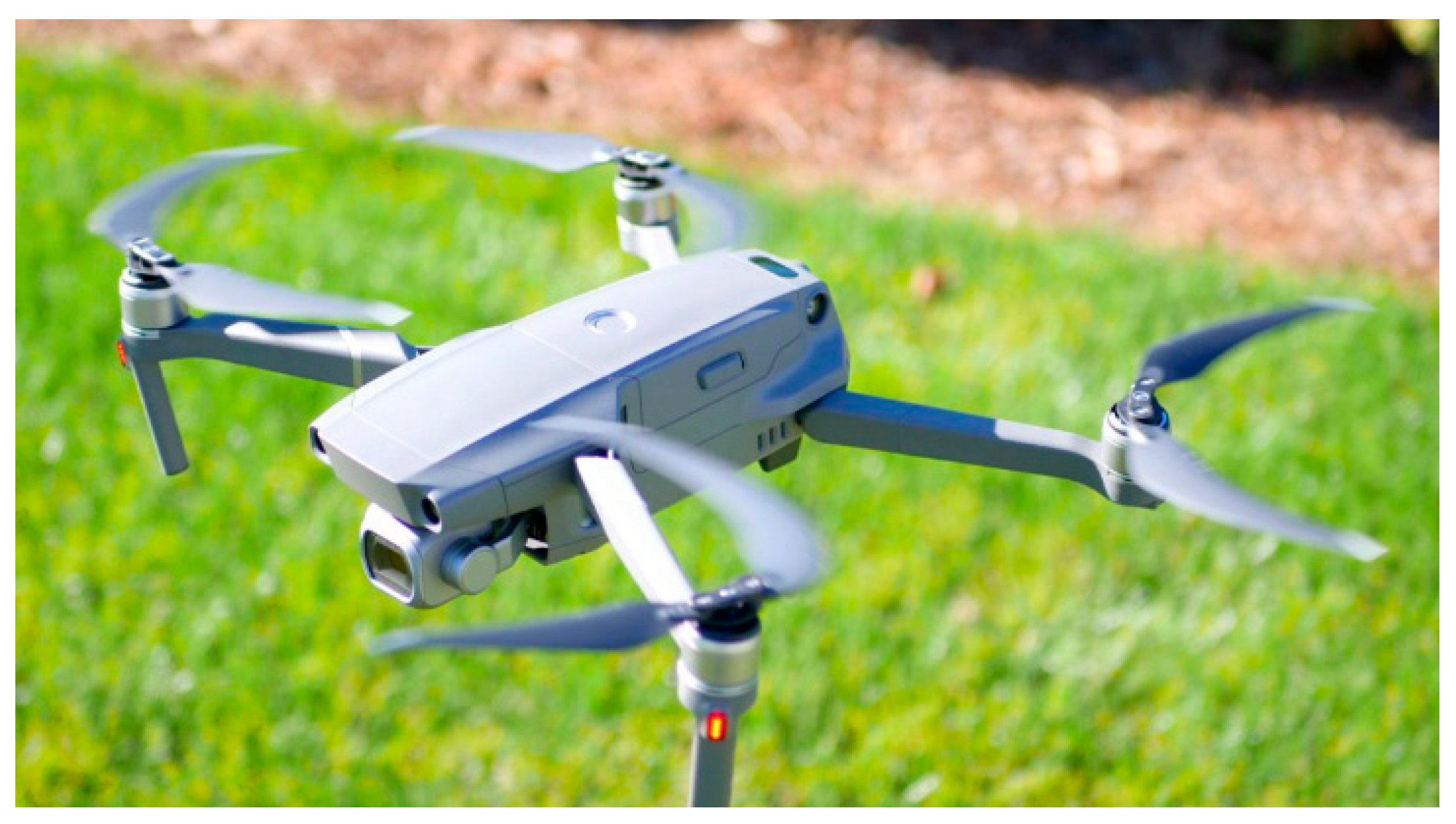
| Camera model | Hasselblad L1D-20c |
| Focal length | 10 mm |
| Aperture | f/2.8 |
| Camera sensor | 1-inch CMOS(13.2 mm × 8.8 mm) |
| Image resolution | 4 K: 3840 × 2160; 2.7 K: 2688 × 1512; FHD: 1920 × 1080 |
| Shooting Mode | Relative Flying Height (m) | GSD (cm) | Shooting Length (m) | Shooting Width (m) | Shooting Area (m2) |
|---|---|---|---|---|---|
| 4K | 100 | Length: 4.64789, Width: 4.07408 | 132 | 88 | 11616 |
| 4K | 150 | Length: 6.97184, Width: 6.11112 | 198 | 132 | 26136 |
| 4K | 200 | Length: 9.29578, Width: 8.14816 | 264 | 176 | 46464 |
| 2.7K | 100 | Length: 4.91072, Width: 5.82011 | 132 | 88 | 11616 |
| 2.7K | 150 | Length: 7.36608, Width: 8.73017 | 198 | 132 | 26136 |
| 2.7K | 200 | Length: 9.82144, Width: 11.6402 | 264 | 176 | 46464 |
| FHD | 100 | Length: 6.87500, Width: 8.14815 | 132 | 88 | 11616 |
| FHD | 150 | Length: 10.3125, Width: 12.2223 | 198 | 132 | 26136 |
| FHD | 200 | Length: 13.7500, Width: 16.2963 | 264 | 176 | 46464 |
Disclaimer/Publisher’s Note: The statements, opinions and data contained in all publications are solely those of the individual author(s) and contributor(s) and not of MDPI and/or the editor(s). MDPI and/or the editor(s) disclaim responsibility for any injury to people or property resulting from any ideas, methods, instructions or products referred to in the content. |
© 2025 by the authors. Licensee MDPI, Basel, Switzerland. This article is an open access article distributed under the terms and conditions of the Creative Commons Attribution (CC BY) license (https://creativecommons.org/licenses/by/4.0/).
Share and Cite
Zheng, B.; Zhou, J.; Hong, Z.; Tang, J.; Huang, X. Vehicle Recognition and Driving Information Detection with UAV Video Based on Improved YOLOv5-DeepSORT Algorithm. Sensors 2025, 25, 2788. https://doi.org/10.3390/s25092788
Zheng B, Zhou J, Hong Z, Tang J, Huang X. Vehicle Recognition and Driving Information Detection with UAV Video Based on Improved YOLOv5-DeepSORT Algorithm. Sensors. 2025; 25(9):2788. https://doi.org/10.3390/s25092788
Chicago/Turabian StyleZheng, Binshuang, Jing Zhou, Zhengqiang Hong, Junyao Tang, and Xiaoming Huang. 2025. "Vehicle Recognition and Driving Information Detection with UAV Video Based on Improved YOLOv5-DeepSORT Algorithm" Sensors 25, no. 9: 2788. https://doi.org/10.3390/s25092788
APA StyleZheng, B., Zhou, J., Hong, Z., Tang, J., & Huang, X. (2025). Vehicle Recognition and Driving Information Detection with UAV Video Based on Improved YOLOv5-DeepSORT Algorithm. Sensors, 25(9), 2788. https://doi.org/10.3390/s25092788