4.1. Driving Cycle Decomposition Approach
Traditional DPR-based power management methods tend to classify driving segments using known continuous driving cycles, and then develop control strategies by identifying the entire driving cycle. However, for a given driving cycle, these methods often include several types of driving segments that are easily overlooked. This is because different driving patterns can exhibit similar driving segments, and the same driving cycle can contain different types of segments. As a result, control strategies developed based on the entire driving cycle may struggle to ensure optimal vehicle performance. To overcome this limitation, a novel classification method is proposed—using a fuzzy neural network to classify driving segments, grouping them according to their characteristics.
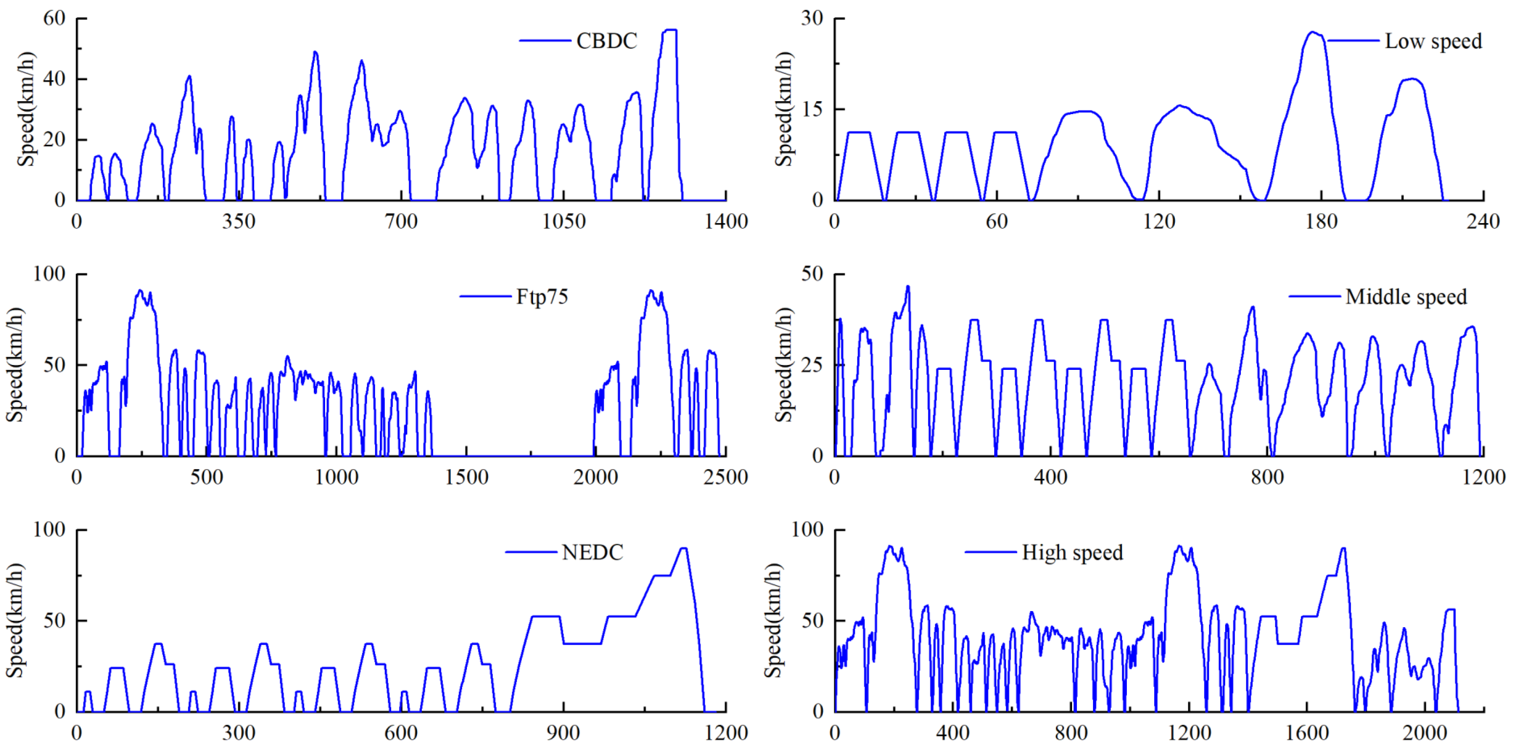
In this study, we selected three typical driving cycles: FTP75, NEDC, and CBDC. For a given driving cycle, the number of parameters used to describe it can reach up to several types. However, too many parameters may significantly increase computation time and could potentially affect the accuracy of the results. In reference [
39], the average speed is reported as the sole parameter. In our research, we use the average speed and maximum speed of each segment as the classification parameters. The methods for calculating average speed and maximum speed are as follows:
where
represents the average speed of each driving segment, where
i denotes the index of the driving segment, and
refers to the maximum speed of each driving segment.
4.2. Fuzzy Neural Network Controller
Driving cycles are crucial for evaluating vehicle performance, especially when calculating fuel economy and emissions. Many standard driving cycles have been developed for different types of vehicles in various countries or scenarios. To better assess the performance of the energy management system (EMS), we designed a driving cycle controller based on a fuzzy neural network.
A fuzzy logic controller is used to classify driving segments and identify the driving types in the DPR process. The controller consists of four key components: fuzzification, rule base, fuzzy inference, and defuzzification. These components work together to effectively process and categorize the driving segments.
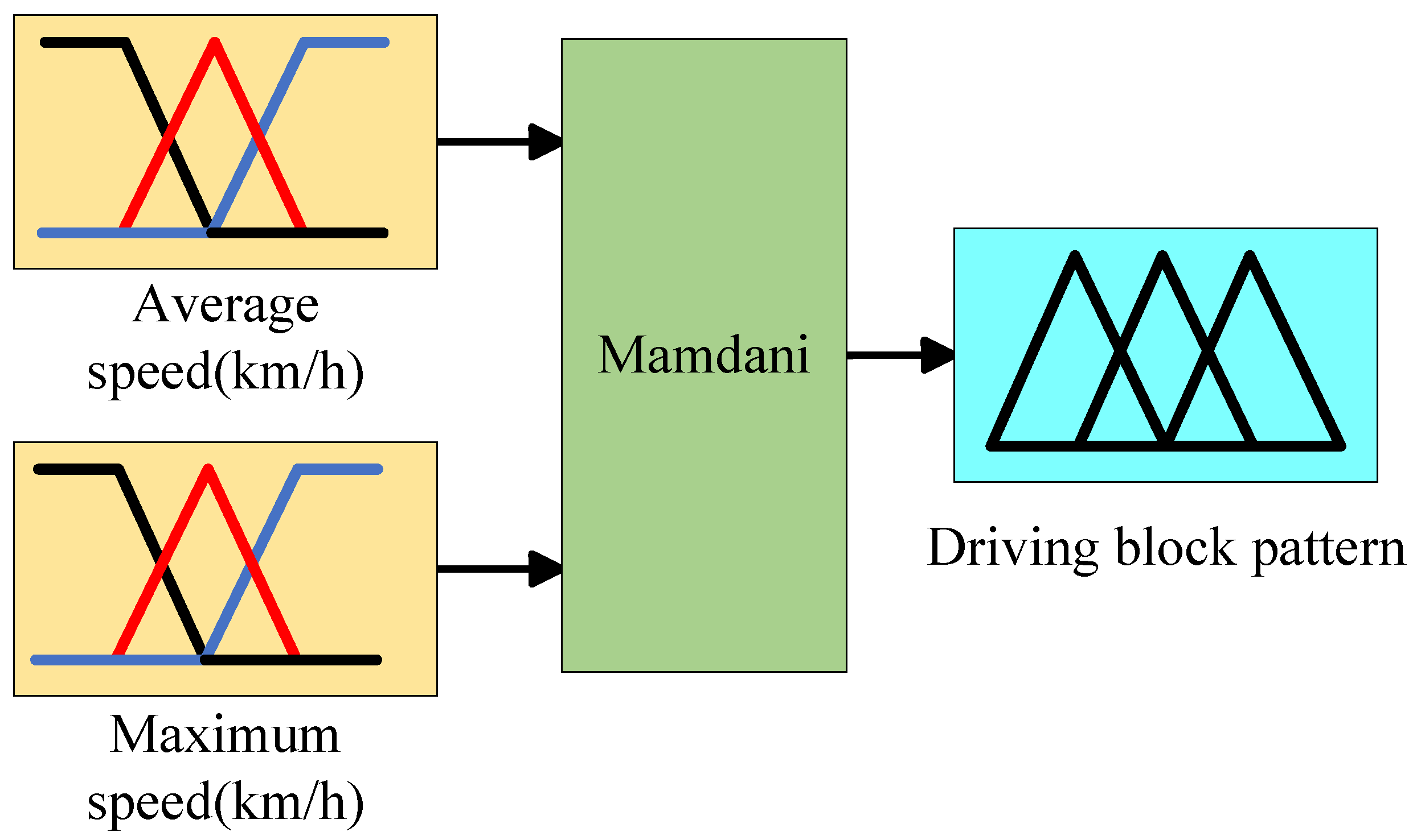
Fuzzification: We set the input variables of the fuzzification module to two parameters: average speed (km/h) and maximum speed (km/h), with the output module being the driving block pattern. For the pre-segmented driving blocks, the average speed and maximum speed are calculated accordingly.
The linguistic terms for the input and output variables are set as Low-Level (low-speed driving pattern), Middle-Level (medium-speed driving pattern), and High-Level (high-speed driving pattern). The inference process utilizes Mamdani’s fuzzy theory. It is noteworthy that, in this study, the intervals corresponding to the three-speed patterns are shown in
Table 4.
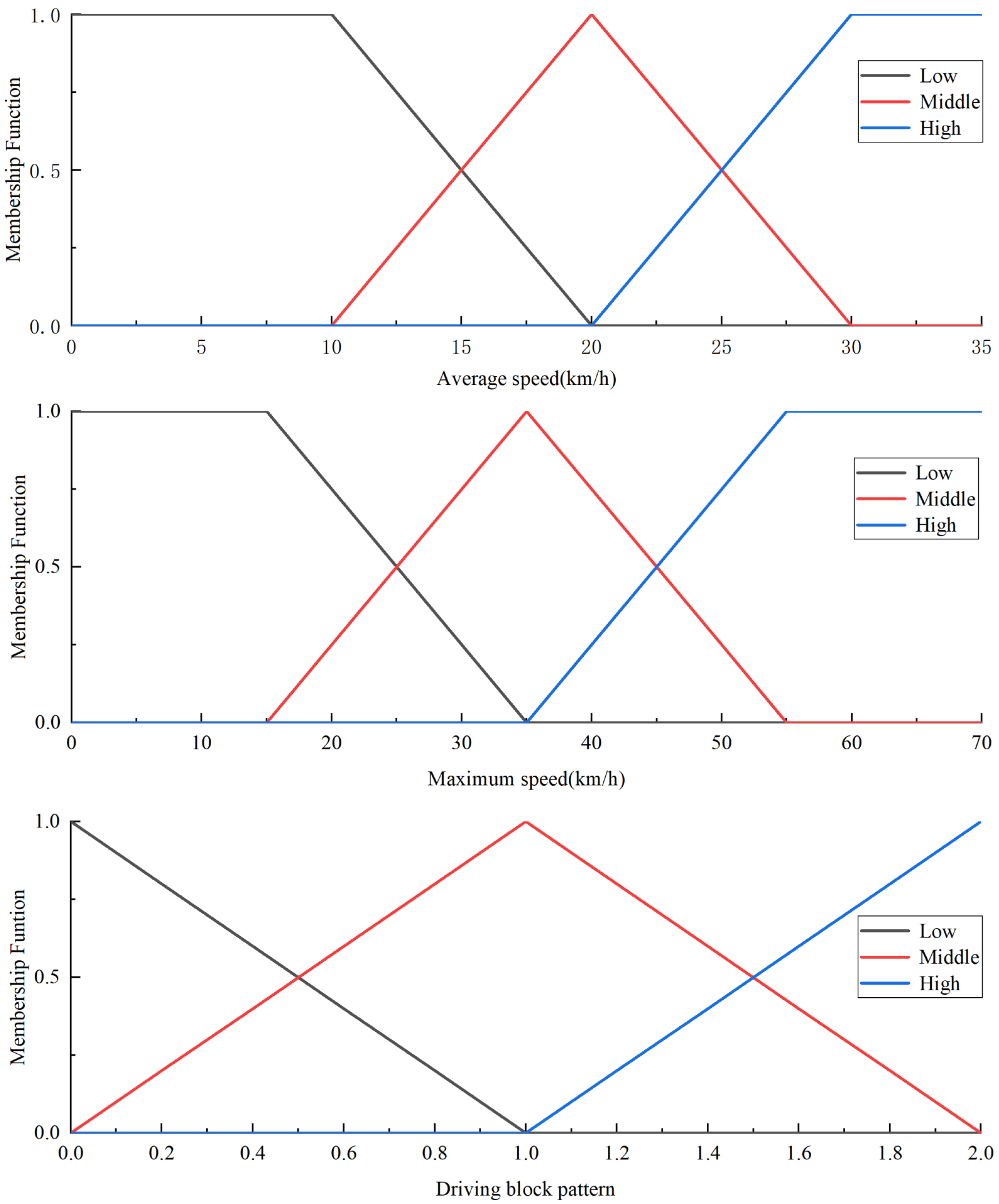
Based on the established rules, we can determine the membership functions for Lower-Level
, Middle-Level
, and High-Level
. The membership function is shown in
Figure 12.
Rule base: The fuzzy logic used in this study follows the
(If A and B, then C) pattern, where A represents the fuzzy set of average speed, which consists of three levels:
,
, and
. B denotes the fuzzy set of maximum speed, which is also divided into three levels:
,
, and
. C represents the fuzzy set of driving block patterns. The inference process is based on the Mamdani fuzzy theory. From each rule shown in
Table 5, we can obtain the corresponding fuzzy relation matrix
through the Cartesian product of
and
. The overall fuzzy relation matrix
R can be obtained by combining the fuzzy relations
using the following equation:
where
m and
n (where
and
) denote the indices of the matrix elements in the fuzzy relation matrix
R and the fuzzy relation matrix
.
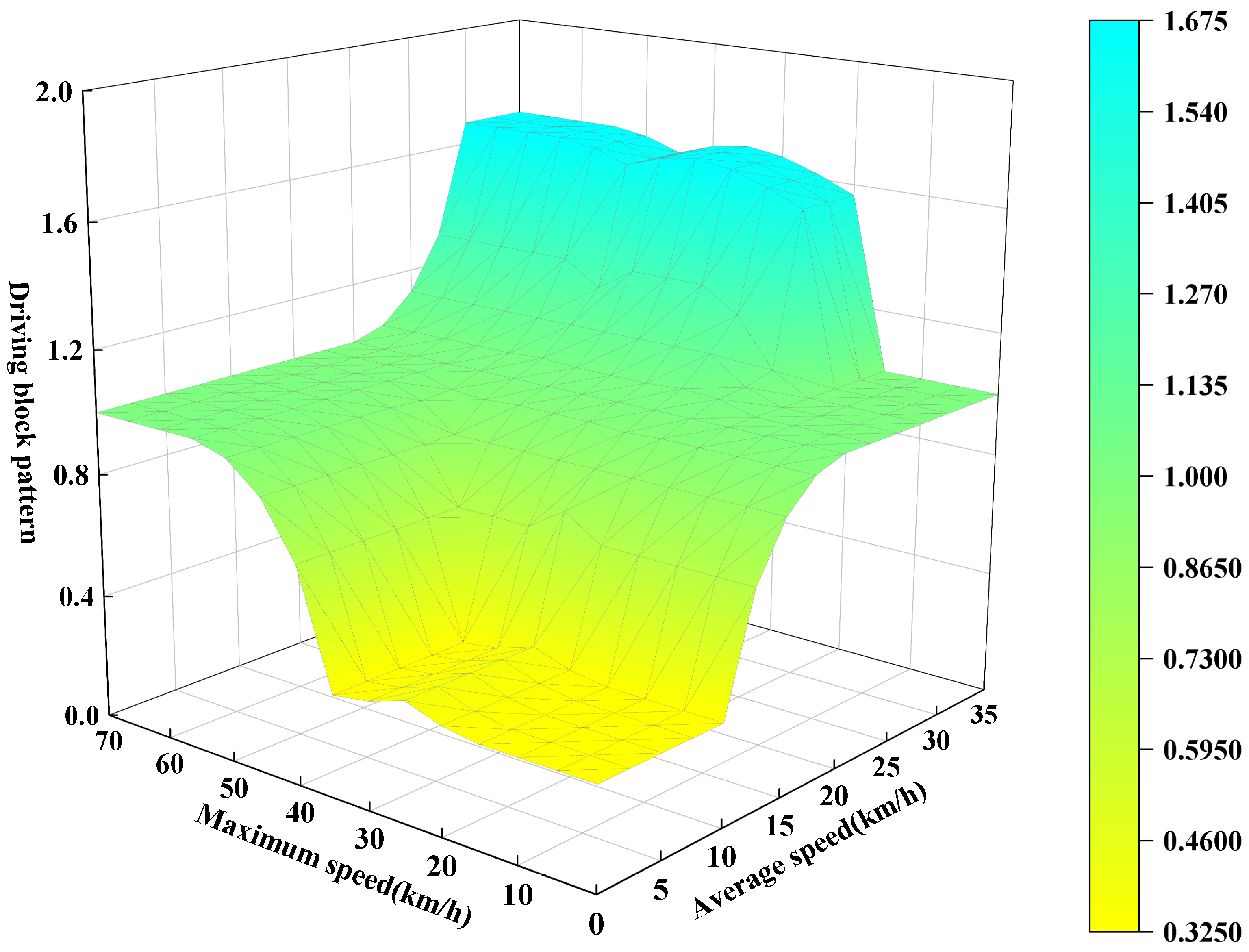
Subsequently, we can examine the three-dimensional coordinate graph of the established fuzzy rules, as shown in
Figure 13.
Fuzzy inference: When we input the fuzzy relation matrix
R of the variables
and
and obtain the fuzzy results, we can use the following equation to determine the driving type:
where
represents the fuzzy set of the output variable.
Defuzzification: The result obtained through the fuzzy set formula is not applicable under real conditions. Therefore, we should convert it to a known driving pattern. The maximum membership principle is employed to determine the driving block pattern. According to this principle, the driving block pattern is identified at the value with the highest membership degree in the domain.
4.4. Speed Prediction Based on LSTM
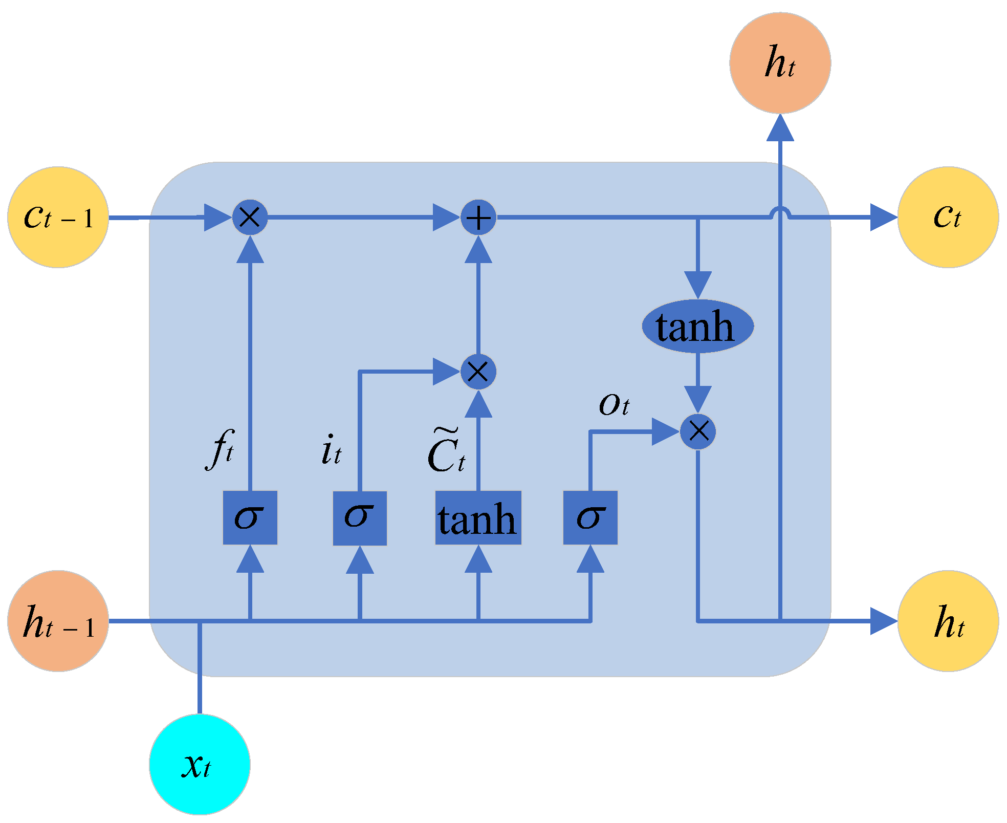
LSTM (Long Short-Term Memory Network) is a commonly used deep learning model for processing sequential data. Compared to traditional RNNs (Recurrent Neural Networks), LSTM introduces three gates (input gate, forget gate, and output gate, as shown in
Figure 17 and a cell state. These mechanisms enable LSTM to better handle long-term dependencies within sequences, with the gates represented by the sigmoid activation function.
Forget Gate: By operating on and and passing the result through the sigmoid function, we obtain a vector in the range of . A value of 0 indicates that a certain portion of the previous memory should be forgotten, while a value of 1 indicates that that portion of the previous memory should be retained.
Input Gate: By adding the information that needs to be retained from the previous state to the information that needs to be remembered from the current state, we obtain the new memory state.
Output Gate: This gate integrates to produce an output.
The calculation formulas for each parameter in the structural diagram are shown in the following equations:
where
is the output value of the forgetting gate;
is the output value of the input gate;
is the output value of the output gate;
is the corresponding gate; and
W is the corresponding parameter.
is the cell state (memory state), is the input information, and is the hidden state (derived from ).
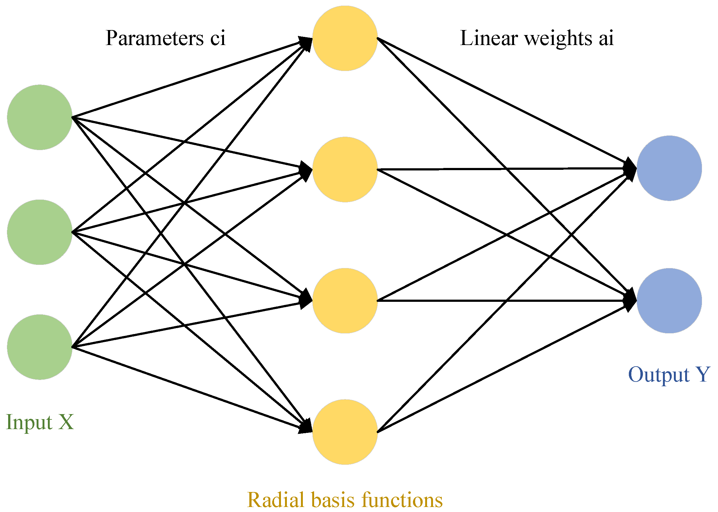
BP (backpropagation) neural network is a multilayer neural network that uses error backpropagation. In systems such as signal processing and pattern recognition, multilayer feedforward networks are widely used models. However, most learning algorithms based on backpropagation for multilayer feedforward networks must rely on some form of nonlinear optimization techniques, which results in large computational costs and slow learning speeds. The theory of Radial Basis Function Neural Network provides a novel and effective means for learning in multilayer feedforward networks. RBF networks not only possess good generalization capabilities but also have lower computational requirements, with learning speeds generally much faster than other algorithms. The following diagram illustrates a simplified model of the RBF network.
After generalization, the applicability is significantly increased. The mapping from the input layer to the hidden layer (radial basis function layer) is a nonlinear mapping, with the basis function being the Gaussian function:
where
;
x is an n-dimensional input vector;
is the center value of the
i-th basis function, which has the same dimensionality as the input vector;
represents the normalization constant of the width of the
i-th basis function’s center; and
is the norm of the vector
, indicating the distance between
x and
. The Gaussian function value
reaches its unique maximum at a specific center value of the basis function. According to the above function, as
increases, the value of the basis function
decreases, approaching zero. For a given input value
, only a small region near the center of
x is activated, the radial basis function is shown in
Figure 18.
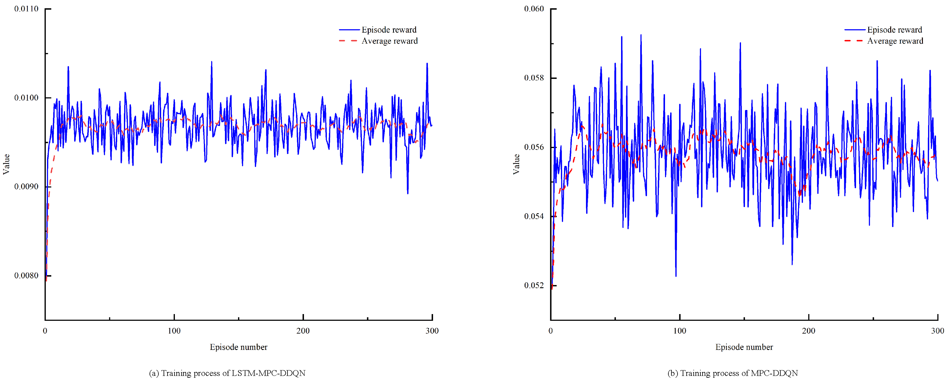
To evaluate the computational complexity of the proposed method, a detailed analysis was conducted to estimate the number of floating-point operations required to compute the control law. The proposed control method consists mainly of the LSTM model and the MPC optimization problem. In the LSTM model, the computational complexity of state estimation is O(n2), where n is the number of neurons in the hidden layer, while during the prediction phase, the complexity is O(n), as only a forward pass is needed to compute the output. In contrast, the MPC controller involves solving an optimization problem, which typically has a complexity of O(n3), where N is the prediction horizon length. By integrating the LSTM and DDQN models into the MPC framework, the proposed method significantly reduces the computational load per control update, eliminating the need for solving large-scale optimization problems at each control step as required by traditional methods.
By comparing the computational complexity of the traditional MPC method with that of the proposed method, we estimate that the number of floating-point operations required for each control update is approximately X operations for the proposed method, compared to Y operations for the traditional MPC method. This demonstrates the clear computational efficiency advantage of the proposed method, particularly in real-time applications where computational burden is a critical factor.


