
A General Numerical Error Compensation Method for NLFM Signal in SAR System Based on Non-Start–Stop Model


Abstract
1. Introduction
2. LFM and NLFM Signal Model and Property
2.1. LFM Signal
2.2. NLFM Signal
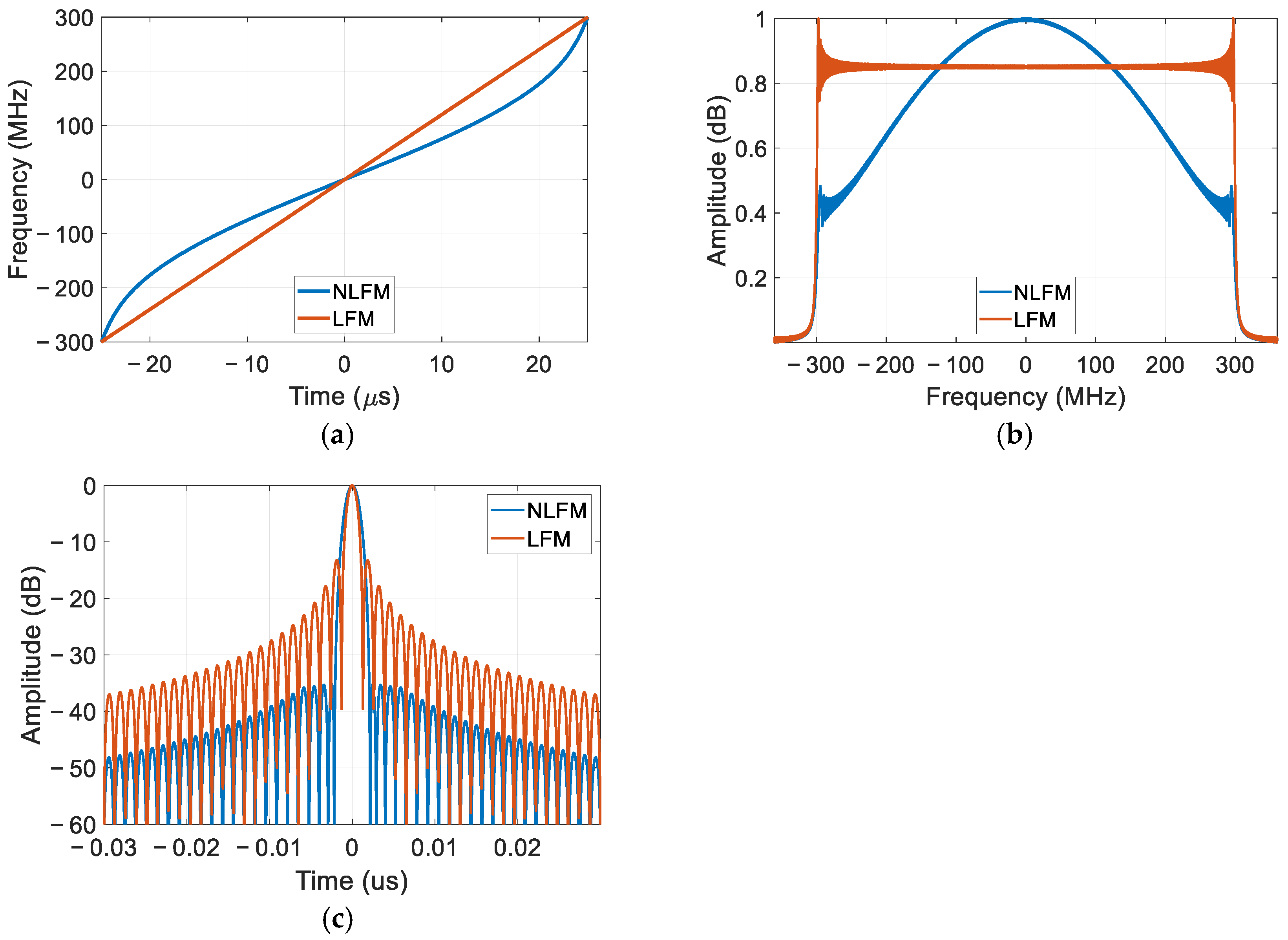
2.3. Comparison Between LFM and NLFM
3. SAR Echo Signal
3.1. Start–Stop Model
3.2. Non-Start–Stop Model
4. Error Analysis and Numerical Compensation Method
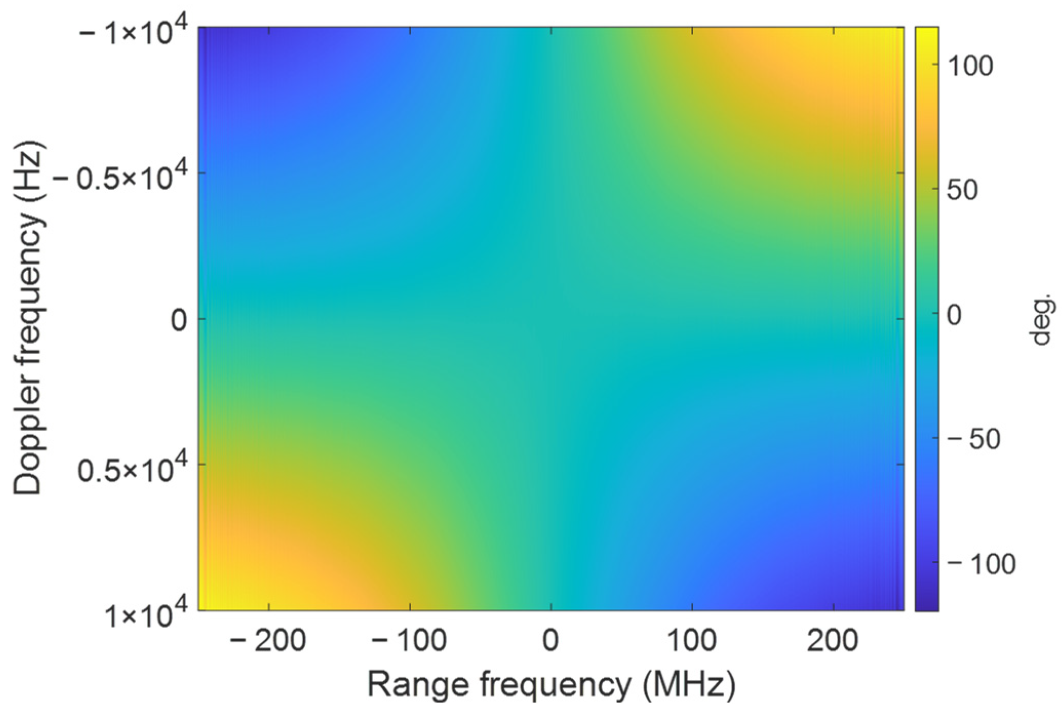
4.1. Error Analysis
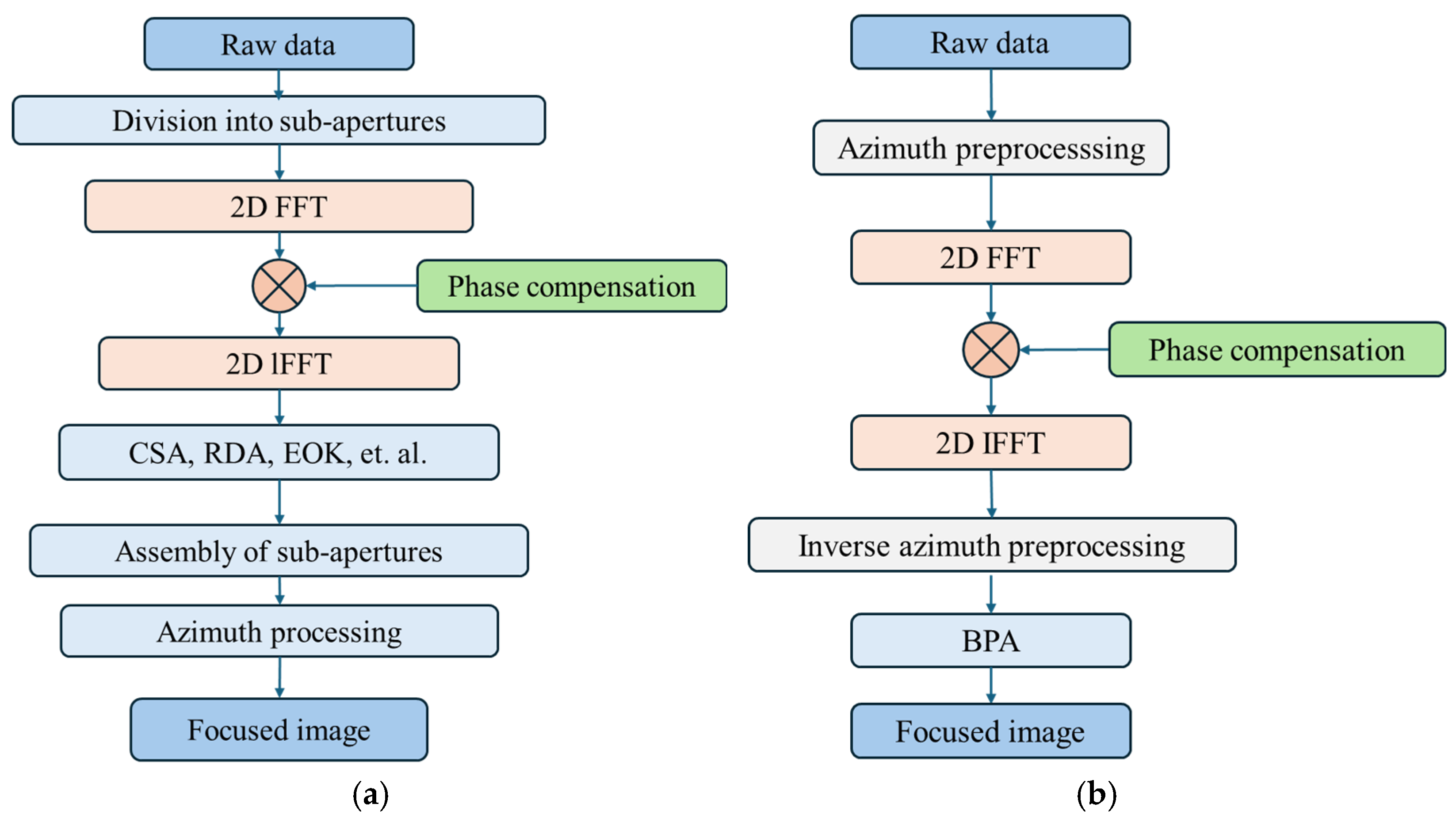
4.2. Proposed Compensation Method
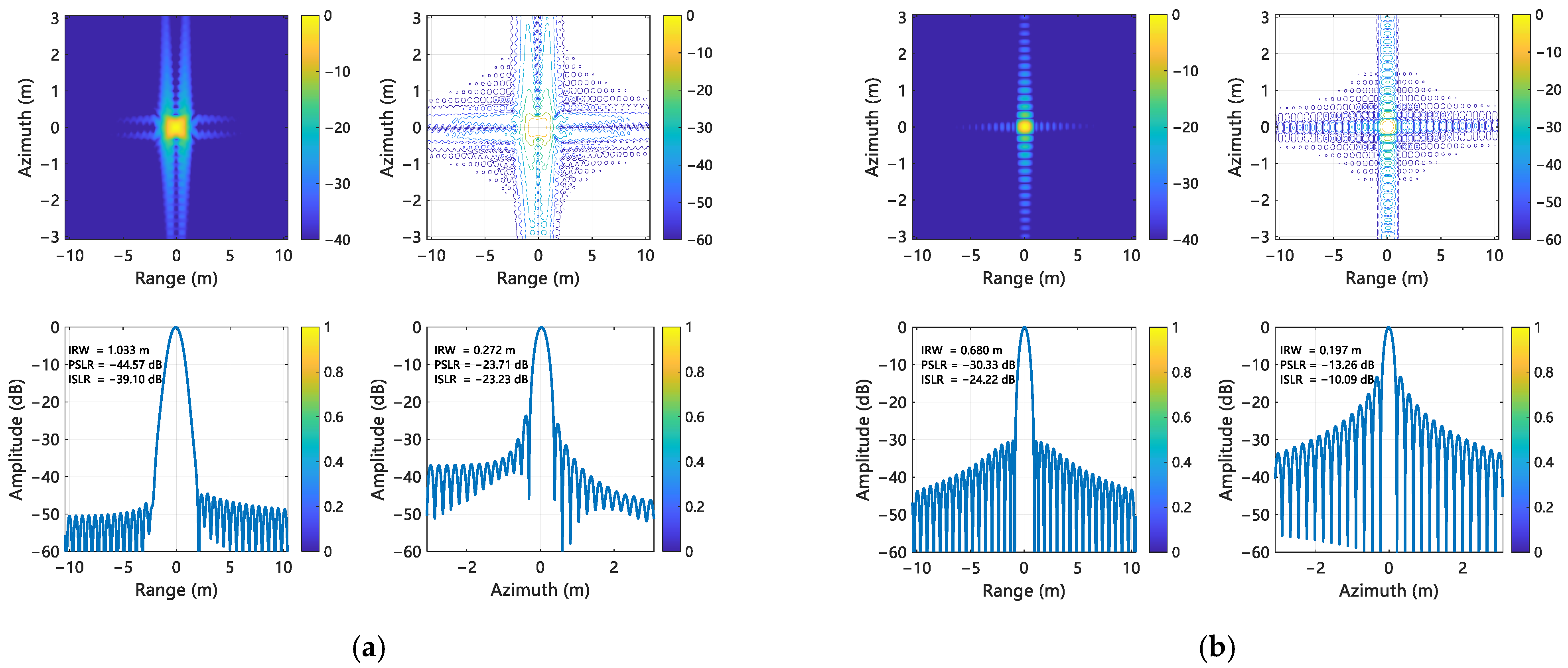
5. Simulation Experiments
6. Conclusions
Author Contributions
Funding
Institutional Review Board Statement
Informed Consent Statement
Data Availability Statement
Conflicts of Interest
Abbreviations
| SAR | synthetic aperture radar |
| LFM | linear frequency modulated |
| NLFM | nonlinear frequency modulated |
| IRW | impulse response width |
| PSLR | peak sidelobe ratio |
| ISLR | integrated sidelobe ratio |
| POSP | principle of stationary phase |
| PSD | power spectral density |
| SNR | signal-to-noise ratio |
| PRI | pulse repetition interval |
| PRF | pulse repetition frequency |
| MIMO | multipe input multiple output |
References
- Moreira, A.; Prats-Iraola, P.; Younis, M.; Krieger, G.; Hajnsek, I.; Papathanassiou, K.P. A Tutorial on Synthetic Aperture Radar. IEEE Geosci. Remote Sens. Mag. 2013, 1, 6–43. [Google Scholar] [CrossRef]
- Deng, Y.; Yu, W.; Wang, P.; Xiao, D.; Wang, W.; Liu, K.; Zhang, H. The High-Resolution Synthetic Aperture Radar System and Signal Processing Techniques: Current Progress and Future Prospects. IEEE Geosci. Remote Sens. Mag. 2024, 12, 169–189. [Google Scholar] [CrossRef]
- Deng, Y.; Zhang, H.; Liu, K.; Wang, W.; Ou, N.; Han, H.; Yang, R.; Ren, J.; Wang, J.; Ren, X.; et al. Hongtu-1: The First Spaceborne Single-Pass MultiBaseline SAR Interferometry Mission. IEEE Trans. Geosci. Remote Sens. 2024, 63, 5202518. [Google Scholar] [CrossRef]
- Lin, Q.; Li, S.; Yu, W. Review on Phase Synchronization Methods for Spaceborne Multistatic Synthetic Aperture Radar. Sensors 2024, 24, 3122. [Google Scholar] [CrossRef]
- Prats-Iraola, P.; Scheiber, R.; Rodriguez-Cassola, M.; Mittermayer, J.; Wollstadt, S.; Zan, F.D.; Brautigam, B.; Schwerdt, M.; Reigber, A.; Moreira, A. On the Processing of Very High Resolution Spaceborne SAR Data. IEEE Trans. Geosci. Remote Sens. 2014, 52, 6003–6016. [Google Scholar] [CrossRef]
- Yan, L.; Xing, M.; Sun, G.; Lv, X.; Zheng, B.; Wen, H.; Wu, Y. Echo Model Analyses and Imaging Algorithm for High-Resolution SAR on High-Speed Platform. IEEE Trans. Geosci. Remote Sens. 2012, 50, 933–950. [Google Scholar]
- Liang, D.; Zhang, H.; Fang, T.; Deng, Y.; Yu, W.; Zhang, L.; Fan, H. Processing of Very High Resolution GF-3 SAR Spotlight Data With Non-Start–Stop Model and Correction of Curved Orbit. IEEE J. Sel. Top. Appl. Earth Observ. Remote Sens. 2020, 13, 2112–2122. [Google Scholar] [CrossRef]
- Liang, D.; Zhang, H.; Fang, T.; Lin, H.; Liu, D.; Jia, X. A Modified Cartesian Factorized Backprojection Algorithm Integrating with Non-Start-Stop Model for High Resolution SAR Imaging. Remote Sens. 2020, 12, 3807. [Google Scholar] [CrossRef]
- Cumming, I.G.; Wong, F.H. Digital Processing of Synthetic Aperture Radar Data: Algorithms and Implementation; Artech House: Norwood, MA, USA, 2005. [Google Scholar]
- Yu, Z.; Wang, S.; Li, Z. An Imaging Compensation Algorithm for Spaceborne High-Resolution SAR Based on a Continuous Tangent Motion Model. Remote Sens. 2016, 8, 223. [Google Scholar] [CrossRef]
- Zhang, Q.; Wu, J.; Qu, J.; Li, Z.; Huang, Y.; Yang, J. Echo Model Without Stop-and-Go Approximation for Bistatic SAR with Maneuvers. IEEE Geosci. Remote Sens. Lett. 2019, 16, 1056–1060. [Google Scholar] [CrossRef]
- Wang, W.; Wang, R.; Deng, Y.; Zhang, Z.; Wu, X.; Xu, Z. Demonstration of NLFM Waveforms With Experiments and Doppler Shift Compensation for SAR Application. IEEE Geosci. Remote Sens. Lett. 2016, 13, 1999–2003. [Google Scholar] [CrossRef]
- Wang, W.; Wang, R.; Zhang, Z.; Deng, Y.; Li, N.; Hou, L.; Xu, Z. First demonstration of airborne SAR with nonlinear FM chirp waveforms. IEEE Geosci. Remote Sens. Lett. 2016, 13, 247–251. [Google Scholar] [CrossRef]
- Doerry, A.W. SAR Processing with Non-Linear FM Chirp Waveforms; Sandia National Laboratories (SNL): Albuquerque, NM, USA; Livermore, CA, USA, 2006.
- Milczarek, H.; Leśnik, C.; Djurović, I.; Kawalec, A. Estimating the instantaneous frequency of linear and nonlinear frequency modulated radar signals—A comparative study. Sensors 2021, 21, 2840. [Google Scholar] [CrossRef] [PubMed]
- Saleh, M.; Omar, S.-M.; Grivel, E.; Legrand, P. A variable chirp rate stepped frequency linear frequency modulation waveform designed to approximate wideband non-linear radar waveforms. Digit. Signal Process. 2021, 109, 102884. [Google Scholar] [CrossRef]
- Song, C.; Wang, Y.; Jin, G.; Wang, Y.; Dong, Q.; Wang, B.; Zhou, L.; Lu, P.; Wu, Y. A novel jamming method against SAR using nonlinear frequency modulation waveform with very high sidelobes. Remote Sens. 2022, 14, 5370. [Google Scholar] [CrossRef]
- Wei, Y.; Liu, Y.; Wang, P.; Zhang, Y.; Qiu, J.; Deng, Y.; Wang, W.; Liu, R.; Zhang, Z.; Li, J. Intermediate-frequency nonlinear frequency modulation signal generator for uav SAR missions. IEEE Geosci. Remote Sens. Lett. 2024, 21, 4007405. [Google Scholar] [CrossRef]
- Zhang, Y.; Deng, Y.; Zhang, Z.; Wang, W.; Lv, Z.; Wei, T.; Wang, R. Analytic NLFM waveform design with harmonic decomposition for synthetic aperture radar. IEEE Geosci. Remote Sens. Lett. 2022, 19, 1–5. [Google Scholar] [CrossRef]
- Jin, G.; Liu, K.; Deng, Y.; Sha, Y.D.; Wang, R.; Liu, D.; Wang, W.; Long, Y.; Zhang, Y. Nonlinear Frequency Modulation Signal Generator in LT-1. IEEE Geosci. Remote Sens. Lett. 2019, 16, 1570–1574. [Google Scholar] [CrossRef]
- Jin, G.; Deng, Y.; Wang, R.; Wang, W.; Wang, P.; Long, Y.; Zhang, Z.M.; Zhang, Y. An advanced nonlinear frequency modulation waveform for radar imaging with low sidelobe. IEEE Trans. Geosci. Remote Sens. 2019, 57, 6155–6168. [Google Scholar] [CrossRef]
- Wei, T.; Wang, W.; Zhang, Y.; Wang, R. A Novel Nonlinear Frequency Modulation Waveform with Low Sidelobes Applied to Synthetic Aperture Radar. IEEE Geosci. Remote Sens. Lett. 2022, 19, 1–5. [Google Scholar] [CrossRef]
- Xu, Z.; Wang, X.; Wang, Y. Nonlinear frequency-modulated waveforms modeling and optimization for radar applications. Mathematics 2022, 10, 3939. [Google Scholar] [CrossRef]
- Han, S.; Deng, Y.; Zhao, Q.; Zhang, Y.; Zhang, Y.; Wang, W. On spaceborne DBF-SAR adopting the degree of freedom with NLFM waveform: Optimization framework and simulation. IEEE Trans. Geosci. Remote Sens. 2022, 60, 1–15. [Google Scholar] [CrossRef]
- Liang, D.; Li, H.; Fu, Y.; Pang, X. A novel transmission loss compensation method for radome based on non-linear frequency modulation waveform design. Electron. Lett. 2023, 59, e12876. [Google Scholar] [CrossRef]
- Jin, G.; Zhang, X.; Huang, J.; Zhu, D. High Freedom Parameterized FM (HFPFM) Code: Model, Correlation Function and Advantages. IEEE Trans. Aerosp. Electron. Syst. 2024, 60, 6284–6298. [Google Scholar] [CrossRef]
- Jin, G.; Aubry, A.; De Maio, A.; Wang, R.; Wang, W. Quasi-Orthogonal Waveforms for Ambiguity Suppression in Spaceborne Quad-Pol SAR. IEEE Trans. Geosci. Remote Sens. 2021, 60, 5204617. [Google Scholar] [CrossRef]
- Akan, A.; Chaparro, L.F. Signals and Systems Using MATLAB®; Elsevier: Amsterdam, The Netherlands, 2024. [Google Scholar]


| Parameter | Value |
|---|---|
| Range bandwidth | 500 MHz |
| Carrier frequency | 10 GHz |
| Pulse duration | 60 μs |
| Sidelobe number | 4 |
| Relative to the mainlobe. | −30 dB |
| Parameter | Value |
|---|---|
| Orbit height | 500 km |
| Carrier frequency | 10 GHz |
| Incidence angle | 30° |
| Range bandwidth | 500 MHz |
| Range sampling frequency | 600 MHz |
| Pulse duration | 60 μs |
| PRF | 5000 Hz |
| Acquisition time | 6.55 s |
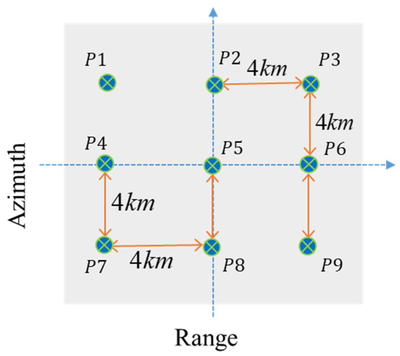
| Targets | Range | Azimuth | ||||
|---|---|---|---|---|---|---|
| IRW (m) | PSLR (dB) | ISLR (dB) | IRW (m) | PSLR (dB) | ISLR (dB) | |
| P1 | 1.033 | −44.57 | −39.10 | 0.272 | −23.71 | −23.23 |
| P2 | 1.013 | −43.17 | −38.41 | 0.272 | −23.15 | −22.42 |
| P3 | 1.068 | −38.82 | −34.82 | 0.292 | −20.69 | −19.58 |
| P4 | 1.018 | −47.45 | −40.60 | 0.270 | −24.00 | −23.63 |
| P5 | 1.089 | −38.16 | −33.47 | 0.299 | −19.51 | −18.33 |
| P6 | 0.998 | −48.17 | −41.15 | 0.270 | −24.07 | −23.74 |
| P7 | 1.081 | −38.65 | −34.37 | 0.294 | −20.40 | −19.36 |
| P8 | 1.229 | −34.03 | −29.57 | 0.354 | −16.23 | −15.06 |
| P9 | 1.003 | −42.82 | −38.13 | 0.274 | −23.46 | −22.88 |
| Targets | Range | Azimuth | ||||
|---|---|---|---|---|---|---|
| IRW (m) | PSLR (dB) | ISLR (dB) | IRW (m) | PSLR (dB) | ISLR (dB) | |
| P1 | 0.680 | −30.33 | −24.22 | 0.197 | −13.26 | −10.09 |
| P2 | 0.675 | −30.32 | −24.21 | 0.197 | −13.26 | −10.09 |
| P3 | 0.669 | −30.34 | −24.20 | 0.198 | −13.26 | −10.09 |
| P4 | 0.680 | −30.32 | −24.18 | 0.197 | −13.26 | −10.09 |
| P5 | 0.674 | −30.32 | −24.17 | 0.197 | −13.26 | −10.08 |
| P6 | 0.669 | −30.30 | −24.16 | 0.198 | −13.26 | −10.09 |
| P7 | 0.680 | −30.29 | −24.22 | 0.197 | −13.26 | −10.09 |
| P8 | 0.675 | −30.29 | −24.21 | 0.197 | −13.26 | −10.09 |
| P9 | 0.669 | −30.31 | −24.20 | 0.198 | −13.26 | −10.09 |
Disclaimer/Publisher’s Note: The statements, opinions and data contained in all publications are solely those of the individual author(s) and contributor(s) and not of MDPI and/or the editor(s). MDPI and/or the editor(s) disclaim responsibility for any injury to people or property resulting from any ideas, methods, instructions or products referred to in the content. |
© 2025 by the authors. Licensee MDPI, Basel, Switzerland. This article is an open access article distributed under the terms and conditions of the Creative Commons Attribution (CC BY) license (https://creativecommons.org/licenses/by/4.0/).
Share and Cite
Wang, G.; Zhang, H.; Li, B.; Yu, W. A General Numerical Error Compensation Method for NLFM Signal in SAR System Based on Non-Start–Stop Model. Sensors 2025, 25, 2770. https://doi.org/10.3390/s25092770
Wang G, Zhang H, Li B, Yu W. A General Numerical Error Compensation Method for NLFM Signal in SAR System Based on Non-Start–Stop Model. Sensors. 2025; 25(9):2770. https://doi.org/10.3390/s25092770
Chicago/Turabian StyleWang, Gui, Heng Zhang, Bo Li, and Weidong Yu. 2025. "A General Numerical Error Compensation Method for NLFM Signal in SAR System Based on Non-Start–Stop Model" Sensors 25, no. 9: 2770. https://doi.org/10.3390/s25092770
APA StyleWang, G., Zhang, H., Li, B., & Yu, W. (2025). A General Numerical Error Compensation Method for NLFM Signal in SAR System Based on Non-Start–Stop Model. Sensors, 25(9), 2770. https://doi.org/10.3390/s25092770