
Impact of Temporal Resolution on Autocorrelative Features of Cerebral Physiology from Invasive and Non-Invasive Sensors in Acute Traumatic Neural Injury: Insights from the CAHR-TBI Cohort

 , , , , , , ,
Abstract
1. Introduction
2. Materials and Methods
2.1. Study Participants
2.2. Data Collection
2.3. Signal Processing
2.4. Data Analysis
2.4.1. Temporal Resolution Reduction
2.4.2. Evaluation of Stationarity
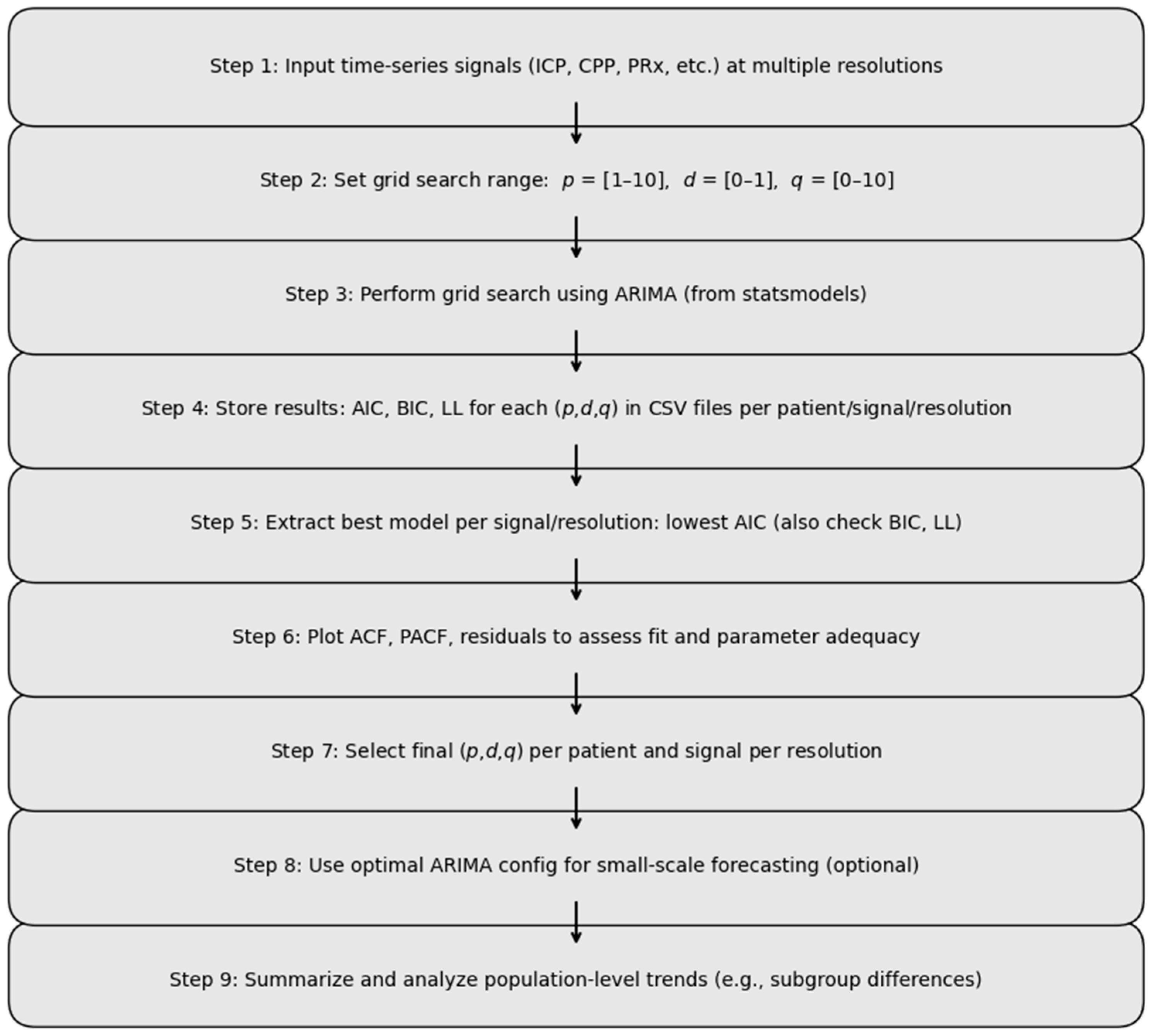
2.4.3. ARIMA Analysis
2.4.4. Subgroup Analysis of ARIMA Model Performance
2.4.5. Forecasting with Optimized ARIMA Parameters—Pilot Analysis
3. Results
3.1. Patient Population
3.2. Results of Evaluation of Stationarity
3.3. ARIMA Analysis Results
3.4. Subgroup Analysis
3.5. Forecasting Results for Optimum ARIMA Parameters—Pilot Analysis
4. Discussion
5. Limitations
6. Conclusions
Supplementary Materials
Author Contributions
Funding
Institutional Review Board Statement
Informed Consent Statement
Data Availability Statement
Acknowledgments
Conflicts of Interest
References
- Sainbhi Khellaf, A.; Khan, D.Z.; Helmy, A. Recent Advances in Traumatic Brain Injury. J. Neurol. 2019, 266, 2878–2889. [Google Scholar] [CrossRef] [PubMed]
- van Erp, I.A.M.; Michailidou, I.; van Essen, T.A.; van der Jagt, M.; Moojen, W.; Peul, W.C.; Baas, F.; Fluiter, K. Tackling Neuroinflammation After Traumatic Brain Injury: Complement Inhibition as a Therapy for Secondary Injury. Neurotherapeutics 2023, 20, 284–303. [Google Scholar] [CrossRef] [PubMed]
- Thapa, K.; Khan, H.; Singh, T.G.; Kaur, A. Traumatic Brain Injury: Mechanistic Insight on Pathophysiology and Potential Therapeutic Targets. J. Mol. Neurosci. 2021, 71, 1725–1742. [Google Scholar] [CrossRef]
- Wang, X.; Feuerstein, G.Z. The Janus Face of Inflammation in Ischemic Brain Injury. In Mechanisms of Secondary Brain Damage from Trauma and Ischemia; Baethmann, A., Eriskat, J., Lehmberg, J., Plesnila, N., Eds.; Springer: Vienna, Austria, 2004; pp. 49–54. [Google Scholar]
- Czosnyka, M.; Miller, C. Monitoring of Cerebral Autoregulation. Neurocrit. Care 2014, 21, 95–102. [Google Scholar] [CrossRef] [PubMed]
- Gritti, P.; Bonfanti, M.; Zangari, R.; Bonanomi, E.; Farina, A.; Pezzetti, G.; Pelliccioli, I.; Longhi, L.; Di Matteo, M.; Viscone, A.; et al. Cerebral Autoregulation in Traumatic Brain Injury: Ultra-Low-Frequency Pressure Reactivity Index and Intracranial Pressure across Age Groups. Crit. Care 2024, 28, 33. [Google Scholar] [CrossRef]
- Easley, R.B.; Kibler, K.K.; Brady, K.M.; Joshi, B.; Ono, M.; Brown, C.; Hogue, C.W. Continuous Cerebrovascular Reactivity Monitoring and Autoregulation Monitoring Identify Similar Lower Limits of Autoregulation in Patients Undergoing Cardiopulmonary Bypass. Neurol. Res. 2013, 35, 344–354. [Google Scholar] [CrossRef]
- Petkus, V.; Preiksaitis, A.; Krakauskaite, S.; Bartusis, L.; Chomskis, R.; Hamarat, Y.; Zubaviciute, E.; Vosylius, S.; Rocka, S.; Ragauskas, A. Non-Invasive Cerebrovascular Autoregulation Assessment Using the Volumetric Reactivity Index: Prospective Study. Neurocrit. Care 2019, 30, 42–50. [Google Scholar] [CrossRef]
- Bernard, F.; Gallagher, C.; Griesdale, D.; Kramer, A.; Sekhon, M.; Zeiler, F.A. The Canadian High-Resolution Traumatic Brain Injury (CAHR-TBI) Research Collaborative. Can. J. Neurol. Sci. 2020, 47, 551–556. [Google Scholar] [CrossRef]
- Zeiler, F.A.; Lee, J.K.; Smielewski, P.; Czosnyka, M.; Brady, K. Validation of Intracranial Pressure-Derived Cerebrovascular Reactivity Indices against the Lower Limit of Autoregulation, Part II: Experimental Model of Arterial Hypotension. J. Neurotrauma 2018, 35, 2812–2819. [Google Scholar] [CrossRef]
- Zeiler, F.A.; Donnelly, J.; Cardim, D.; Menon, D.K.; Smielewski, P.; Czosnyka, M. ICP Versus Laser Doppler Cerebrovascular Reactivity Indices to Assess Brain Autoregulatory Capacity. Neurocrit. Care 2018, 28, 194–202. [Google Scholar] [CrossRef]
- Depreitere, B.; Citerio, G.; Smith, M.; Adelson, P.D.; Aries, M.J.; Bleck, T.P.; Bouzat, P.; Chesnut, R.; De Sloovere, V.; Diringer, M.; et al. Cerebrovascular Autoregulation Monitoring in the Management of Adult Severe Traumatic Brain Injury: A Delphi Consensus of Clinicians. Neurocrit. Care 2021, 34, 731–738. [Google Scholar] [CrossRef] [PubMed]
- Meyer, A.; Zverinski, D.; Pfahringer, B.; Kempfert, J.; Kuehne, T.; Sündermann, S.H.; Stamm, C.; Hofmann, T.; Falk, V.; Eickhoff, C. Machine Learning for Real-Time Prediction of Complications in Critical Care: A Retrospective Study. Lancet Respir. Med. 2018, 6, 905–914. [Google Scholar] [CrossRef]
- Mao, Y.; Chen, W.; Chen, Y.; Lu, C.; Kollef, M.; Bailey, T. An Integrated Data Mining Approach to Real-Time Clinical Monitoring and Deterioration Warning. In Proceedings of the 18th ACM SIGKDD International Conference on Knowledge Discovery and Data Mining, Beijing, China, 12–16 August 2012; Association for Computing Machinery: New York, NY, USA, 2012; pp. 1140–1148. [Google Scholar]
- Jacono, F.J.; De Georgia, M.A.; Wilson, C.G.; Dick, T.E.; Loparo, K.A. Data Acquisition and Complex Systems Analysis in Critical Care: Developing the Intensive Care Unit of the Future. J. Healthc. Eng. 2010, 1, 478492. [Google Scholar] [CrossRef]
- Foreman, B.; Lissak, I.A.; Kamireddi, N.; Moberg, D.; Rosenthal, E.S. Challenges and Opportunities in Multimodal Monitoring and Data Analytics in Traumatic Brain Injury. Curr. Neurol. Neurosci. Rep. 2021, 21, 6. [Google Scholar] [CrossRef] [PubMed]
- Akrami, S.A.; El-Shafie, A.; Naseri, M.; Santos, C.A.G. Rainfall Data Analyzing Using Moving Average (MA) Model and Wavelet Multi-Resolution Intelligent Model for Noise Evaluation to Improve the Forecasting Accuracy. Neural Comput. Applic. 2014, 25, 1853–1861. [Google Scholar] [CrossRef]
- Ma, M.; Zhang, Z.; Zhai, Z.; Zhong, Z. Sparsity-Constrained Vector Autoregressive Moving Average Models for Anomaly Detection of Complex Systems with Multisensory Signals. Mathematics 2024, 12, 1304. [Google Scholar] [CrossRef]
- Chang, C.-H.; Ko, H.-J.; Chang, K.-M. Cancellation of High-Frequency Noise in ECG Signals Using Adaptive Filter without External Reference. In Proceedings of the 2010 3rd International Conference on Biomedical Engineering and Informatics, Yantai, China, 16–18 October 2010; Volume 2, pp. 787–790. [Google Scholar]
- Sainbhi, A.S.; Vakitbilir, N.; Gomez, A.; Stein, K.Y.; Froese, L.; Zeiler, F.A. Time-Series Autocorrelative Structure of Cerebrovascular Reactivity Metrics in Severe Neural Injury: An Evaluation of the Impact of Data Resolution. Biomed. Signal Process. Control 2024, 95, 106403. [Google Scholar] [CrossRef]
- Capan, M.; Hoover, S.; Jackson, E.V.; Paul, D.; Locke, R. Time Series Analysis for Forecasting Hospital Census: Application to the Neonatal Intensive Care Unit. Appl. Clin. Inf. 2016, 7, 275–289. [Google Scholar] [CrossRef]
- Zeiler, F.A.; Aries, M.; Cabeleira, M.; van Essen, T.A.; Stocchetti, N.; Menon, D.K.; Timofeev, I.; Czosnyka, M.; Smielewski, P.; Hutchinson, P.; et al. Statistical Cerebrovascular Reactivity Signal Properties after Secondary Decompressive Craniectomy in Traumatic Brain Injury: A CENTER-TBI Pilot Analysis. J. Neurotrauma 2020, 37, 1306–1314. [Google Scholar] [CrossRef]
- Calviello, L.A.; Czigler, A.; Zeiler, F.A.; Smielewski, P.; Czosnyka, M. Validation of Non-Invasive Cerebrovascular Pressure Reactivity and Pulse Amplitude Reactivity Indices in Traumatic Brain Injury. Acta Neurochir. 2020, 162, 337–344. [Google Scholar] [CrossRef] [PubMed]
- Calviello, L.; Donnelly, J.; Cardim, D.; Robba, C.; Zeiler, F.A.; Smielewski, P.; Czosnyka, M. Compensatory-Reserve-Weighted Intracranial Pressure and Its Association with Outcome After Traumatic Brain Injury. Neurocrit. Care 2018, 28, 212–220. [Google Scholar] [CrossRef]
- Zeiler, F.A.; Ercole, A.; Cabeleira, M.; Carbonara, M.; Stocchetti, N.; Menon, D.K.; Smielewski, P.; Czosnyka, M.; Anke, A.; Beer, R.; et al. Comparison of Performance of Different Optimal Cerebral Perfusion Pressure Parameters for Outcome Prediction in Adult Traumatic Brain Injury: A Collaborative European NeuroTrauma Effectiveness Research in Traumatic Brain Injury (CENTER-TBI) Study. J. Neurotrauma 2019, 36, 1505–1517. [Google Scholar] [CrossRef] [PubMed]
- van Greunen, J.; Heymans, A.; van Heerden, C.; van Vuuren, G. The Prominence of Stationarity in Time Series Forecasting. Stud. Econ. Econom. 2014, 38, 1–16. [Google Scholar] [CrossRef]
- Ho, S.L.; Xie, M.; Goh, T.N. A Comparative Study of Neural Network and Box-Jenkins ARIMA Modeling in Time Series Prediction. Comput. Ind. Eng. 2002, 42, 371–375. [Google Scholar] [CrossRef]
- Shumway, R.H.; Stoffer, D.S. ARIMA Models. In Time Series Analysis and Its Applications: With R Examples; Shumway, R.H., Stoffer, D.S., Eds.; Springer International Publishing: Cham, Switzerland, 2017; pp. 75–163. ISBN 978-3-319-52452-8. [Google Scholar]
- Hassani, H.; Royer-Carenzi, M.; Mashhad, L.M.; Yarmohammadi, M.; Yeganegi, M.R. Exploring the Depths of the Autocorrelation Function: Its Departure from Normality. Information 2024, 15, 449. [Google Scholar] [CrossRef]
- Singh, M. Modified Pennes Bioheat Equation with Heterogeneous Blood Perfusion: A Newer Perspective. Int. J. Heat Mass Transf. 2024, 218, 124698. [Google Scholar] [CrossRef]


| Variable | Median (Interquartile Range) or Number (%) |
|---|---|
| Number of patients | 376 |
| Duration of recording (minutes) | 5904 (3204–11,160) |
| Age (years) | 38 (24–55) |
| Male sex | 288 (78%) |
| GCS | 6 (4–7) |
| GCS-motor | 4 (1–5) |
| Pupils | |
| Bilateral reactive | 185 (50.11%) |
| Bilateral unreactive | 111 (30.01%) |
| Unilateral unreactive | 63 (17.07%) |
| Marshall CT Classification | |
| V + VI | 112 (30.35%) |
| IV | 85 (23.03%) |
| III | 43 (11.65%) |
| II | 100 (27.10%) |
| Hypoxic episode | 61 (26.50%) |
| Hypotensive episode | 35 (15.08%) |
| Mean MAP (mmHg) | 86.9 (81.1–92.9) |
| Mean ICP (mmHg) | 11.9 (8.17–14.8) |
| Temporal Resolution | 1-min | 5-min | 10-min | 30-min | 1-h | 2-h | 3-h | 4-h | 5-h | 6-h | 12-h | 1-day | |
|---|---|---|---|---|---|---|---|---|---|---|---|---|---|
| MAP | Stationarity | 14.5 | 22.3 | 29.7 | 44.8 | 53.5 | 62.1 | 67.6 | 70.1 | 67.8 | 72.3 | 78.7 | 88.9 |
| Non-stationary | 85.2 | 77.4 | 70.0 | 55.0 | 46.2 | 37.6 | 32.1 | 29.6 | 31.9 | 27.4 | 20.9 | 10.6 | |
| NA | 0.3 | 0.3 | 0.3 | 0.3 | 0.3 | 0.3 | 0.3 | 0.3 | 0.3 | 0.3 | 0.4 | 0.5 | |
| ICP | Stationarity | 10.3 | 24.0 | 30.8 | 44.5 | 50.6 | 58.9 | 63.5 | 67.1 | 71.1 | 72.3 | 80.1 | 87.5 |
| Non-stationary | 89.7 | 76.0 | 69.2 | 55.5 | 49.4 | 41.1 | 36.5 | 32.9 | 28.9 | 27.7 | 19.9 | 12.5 | |
| NA | 0.0 | 0.0 | 0.0 | 0.0 | 0.0 | 0.0 | 0.0 | 0.0 | 0.0 | 0.0 | 0.0 | 0.0 | |
| CPP | Stationarity | 15.9 | 30.7 | 38.9 | 49.9 | 55.5 | 64.7 | 68.2 | 71.0 | 71.1 | 72.6 | 79.8 | 87.0 |
| Non-stationary | 83.8 | 69.0 | 60.8 | 49.9 | 44.2 | 35.0 | 31.5 | 28.7 | 28.6 | 27.1 | 19.9 | 12.5 | |
| NA | 0.3 | 0.3 | 0.3 | 0.3 | 0.3 | 0.3 | 0.3 | 0.3 | 0.3 | 0.3 | 0.4 | 0.5 | |
| PRx | Stationarity | 18.1 | 28.2 | 33.6 | 46.5 | 56.1 | 62.4 | 66.8 | 72.5 | 73.9 | 77.3 | 82.6 | 88.4 |
| Non-stationary | 81.6 | 71.5 | 66.1 | 53.3 | 43.6 | 37.3 | 32.9 | 27.2 | 25.8 | 22.4 | 17.0 | 11.1 | |
| NA | 0.3 | 0.3 | 0.3 | 0.3 | 0.3 | 0.3 | 0.3 | 0.3 | 0.3 | 0.3 | 0.4 | 0.5 | |
| PAx | Stationarity | 18.1 | 25.1 | 32.2 | 45.6 | 56.4 | 65.9 | 70.0 | 72.2 | 72.9 | 77.9 | 83.3 | 90.7 |
| Non-stationary | 81.6 | 74.6 | 67.5 | 54.1 | 43.4 | 33.8 | 29.7 | 27.5 | 26.7 | 21.8 | 16.3 | 8.8 | |
| NA | 0.3 | 0.3 | 0.3 | 0.3 | 0.3 | 0.3 | 0.3 | 0.3 | 0.3 | 0.3 | 0.4 | 0.5 | |
| RAC | Stationarity | 15.6 | 23.7 | 31.1 | 41.1 | 50.0 | 60.9 | 65.6 | 69.2 | 72.0 | 75.1 | 81.9 | 89.4 |
| Non-stationary | 84.1 | 76.0 | 68.6 | 58.6 | 49.7 | 38.8 | 34.1 | 30.5 | 27.7 | 24.6 | 17.7 | 10.2 | |
| NA | 0.3 | 0.3 | 0.3 | 0.3 | 0.3 | 0.3 | 0.3 | 0.3 | 0.3 | 0.3 | 0.4 | 0.5 | |
| RAP | Stationarity | 18.9 | 28.8 | 34.5 | 45.6 | 53.5 | 62.7 | 67.1 | 71.3 | 72.6 | 75.4 | 80.9 | 88.9 |
| Non-stationary | 81.1 | 71.2 | 65.5 | 54.4 | 46.5 | 37.3 | 32.9 | 28.7 | 27.4 | 24.6 | 19.1 | 11.1 | |
| NA | 0.0 | 0.0 | 0.0 | 0.0 | 0.0 | 0.0 | 0.0 | 0.0 | 0.0 | 0.0 | 0.0 | 0.0 | |
| COx_L | Stationarity | 13.1 | 15.6 | 17.6 | 21.5 | 24.3 | 25.7 | 25.9 | 27.2 | 28.0 | 28.0 | 27.0 | 27.8 |
| Non-stationary | 24.0 | 21.5 | 19.3 | 14.7 | 11.3 | 9.9 | 9.4 | 8.1 | 7.6 | 6.9 | 4.6 | 2.3 | |
| NA | 63.0 | 62.8 | 63.0 | 63.7 | 64.5 | 64.4 | 64.7 | 64.7 | 64.4 | 65.1 | 68.4 | 69.9 | |
| COx_R | Stationarity | 13.6 | 17.3 | 20.2 | 22.7 | 22.5 | 26.2 | 27.4 | 27.8 | 28.9 | 27.7 | 28.4 | 26.4 |
| Non-stationary | 23.4 | 19.8 | 16.8 | 13.6 | 13.0 | 9.0 | 7.6 | 7.2 | 6.4 | 6.9 | 3.5 | 3.7 | |
| NA | 63.0 | 62.8 | 63.0 | 63.7 | 64.5 | 64.7 | 65.0 | 65.0 | 64.7 | 65.4 | 68.1 | 69.9 | |
| COx-a_L | Stationarity | 14.5 | 17.0 | 17.1 | 21.2 | 21.4 | 23.0 | 25.3 | 25.7 | 25.2 | 26.2 | 27.0 | 26.4 |
| Non-stationary | 21.4 | 19.0 | 18.8 | 13.9 | 13.0 | 11.4 | 8.8 | 8.4 | 9.1 | 7.5 | 3.5 | 3.2 | |
| NA | 64.1 | 64.0 | 64.1 | 64.9 | 65.6 | 65.6 | 65.9 | 65.9 | 65.7 | 66.4 | 69.5 | 70.4 | |
| COx-a_R | Stationarity | 17.0 | 20.1 | 21.3 | 21.8 | 22.0 | 24.5 | 26.2 | 27.2 | 26.7 | 26.2 | 26.6 | 27.3 |
| Non-stationary | 18.9 | 15.9 | 14.6 | 13.3 | 12.4 | 9.6 | 7.6 | 6.6 | 7.3 | 7.2 | 4.3 | 2.3 | |
| NA | 64.1 | 64.0 | 64.1 | 64.9 | 65.6 | 65.9 | 66.2 | 66.2 | 66.0 | 66.7 | 69.1 | 70.4 | |
| rSO2_L | Stationarity | 2.8 | 7.8 | 10.4 | 14.4 | 15.3 | 16.9 | 20.3 | 21.6 | 21.3 | 23.4 | 23.0 | 23.6 |
| Non-stationary | 34.5 | 29.6 | 26.9 | 22.1 | 20.5 | 18.7 | 15.0 | 13.8 | 14.3 | 11.5 | 8.5 | 6.5 | |
| NA | 62.7 | 62.6 | 62.7 | 63.5 | 64.2 | 64.4 | 64.7 | 64.7 | 64.4 | 65.1 | 68.4 | 69.9 | |
| rSO2_R | Stationarity | 4.5 | 10.1 | 11.8 | 15.0 | 17.6 | 19.5 | 22.4 | 22.5 | 22.8 | 23.7 | 25.2 | 23.6 |
| Non-stationary | 32.6 | 27.1 | 25.2 | 21.2 | 17.9 | 15.7 | 12.6 | 12.6 | 12.5 | 10.9 | 6.7 | 6.5 | |
| NA | 63.0 | 62.8 | 63.0 | 63.7 | 64.5 | 64.7 | 65.0 | 65.0 | 64.7 | 65.4 | 68.1 | 69.9 | |
| PbtO2 | Stationarity | 4.7 | 10.1 | 12.0 | 14.4 | 15.3 | 18.4 | 20.6 | 21.3 | 21.6 | 22.1 | 24.1 | 27.8 |
| Non-stationary | 25.1 | 19.6 | 17.6 | 15.0 | 13.9 | 11.1 | 8.8 | 7.2 | 6.7 | 6.5 | 5.0 | 3.7 | |
| NA | 70.2 | 70.4 | 70.3 | 70.5 | 70.8 | 70.6 | 70.6 | 71.6 | 71.7 | 71.3 | 70.9 | 68.5 | |
| Temporal Resolution | 1-min | 5-min | 10-min | 30-min | 1-h | 2-h | 3-h | 4-h | 5-h | 6-h | 12-h | 1-day | |
|---|---|---|---|---|---|---|---|---|---|---|---|---|---|
| MAP | Stationarity | 97.1 | 98.4 | 97.6 | 95.5 | 93.6 | 88.0 | 86.4 | 84.0 | 82.4 | 81.4 | 68.1 | 44.4 |
| Non-stationary | 2.7 | 1.3 | 1.9 | 4.0 | 4.8 | 9.3 | 9.8 | 10.6 | 10.1 | 9.3 | 11.2 | 12.0 | |
| NA | 0.3 | 0.3 | 0.5 | 0.5 | 1.6 | 2.7 | 3.7 | 5.3 | 7.4 | 9.3 | 20.7 | 43.6 | |
| ICP | Stationarity | 92.3 | 94.7 | 97.1 | 95.2 | 92.3 | 87.8 | 87.0 | 85.1 | 81.9 | 81.1 | 66.2 | 44.4 |
| Non-stationary | 7.4 | 5.1 | 2.4 | 4.0 | 5.3 | 9.0 | 8.8 | 8.5 | 10.1 | 8.5 | 11.2 | 10.4 | |
| NA | 0.3 | 0.3 | 0.5 | 0.8 | 2.4 | 3.2 | 4.3 | 6.4 | 8.0 | 10.4 | 22.6 | 45.2 | |
| CPP | Stationarity | 94.7 | 95.7 | 96.8 | 95.7 | 90.2 | 87.0 | 83.2 | 81.6 | 81.1 | 78.7 | 63.8 | 42.6 |
| Non-stationary | 4.8 | 3.7 | 2.4 | 3.2 | 6.9 | 8.8 | 11.4 | 10.9 | 9.8 | 9.6 | 12.8 | 11.7 | |
| NA | 0.5 | 0.5 | 0.8 | 1.1 | 2.9 | 4.3 | 5.3 | 7.4 | 9.0 | 11.7 | 23.4 | 45.7 | |
| PRx | Stationarity | 97.9 | 96.3 | 96.3 | 92.8 | 89.6 | 87.8 | 86.2 | 82.2 | 75.8 | 76.1 | 62.8 | 42.6 |
| Non-stationary | 1.6 | 3.2 | 2.9 | 6.1 | 7.4 | 8.0 | 8.5 | 10.1 | 15.2 | 12.5 | 13.8 | 11.2 | |
| NA | 0.5 | 0.5 | 0.8 | 1.1 | 2.9 | 4.3 | 5.3 | 7.7 | 9.0 | 11.4 | 23.4 | 46.3 | |
| PAx | Stationarity | 98.4 | 94.7 | 96.0 | 91.8 | 87.8 | 85.9 | 83.5 | 80.6 | 80.3 | 79.0 | 60.9 | 41.2 |
| Non-stationary | 1.1 | 4.8 | 3.2 | 7.2 | 9.3 | 9.8 | 11.2 | 11.7 | 10.6 | 9.6 | 15.7 | 12.5 | |
| NA | 0.5 | 0.5 | 0.8 | 1.1 | 2.9 | 4.3 | 5.3 | 7.7 | 9.0 | 11.4 | 23.4 | 46.3 | |
| RAC | Stationarity | 98.1 | 96.3 | 94.9 | 91.8 | 88.8 | 87.5 | 83.5 | 80.1 | 79.8 | 79.5 | 63.0 | 39.6 |
| Non-stationary | 1.3 | 3.2 | 4.3 | 7.2 | 8.2 | 8.2 | 11.2 | 12.2 | 11.2 | 9.0 | 13.6 | 14.1 | |
| NA | 0.5 | 0.5 | 0.8 | 1.1 | 2.9 | 4.3 | 5.3 | 7.7 | 9.0 | 11.4 | 23.4 | 46.3 | |
| RAP | Stationarity | 98.1 | 95.7 | 95.2 | 93.4 | 89.1 | 84.8 | 86.4 | 81.6 | 77.4 | 77.4 | 61.4 | 43.6 |
| Non-stationary | 1.6 | 4.0 | 4.3 | 5.9 | 8.5 | 12.0 | 9.3 | 12.0 | 14.4 | 12.2 | 16.0 | 10.9 | |
| NA | 0.3 | 0.3 | 0.5 | 0.8 | 2.4 | 3.2 | 4.3 | 6.4 | 8.2 | 10.4 | 22.6 | 45.5 | |
| COx_L | Stationarity | 29.5 | 30.1 | 29.5 | 27.4 | 28.2 | 25.8 | 26.1 | 24.2 | 23.9 | 22.3 | 20.2 | 12.5 |
| Non-stationary | 1.1 | 0.3 | 0.3 | 2.1 | 0.8 | 2.7 | 1.9 | 3.2 | 2.4 | 3.5 | 2.9 | 5.6 | |
| NA | 69.4 | 69.7 | 70.2 | 70.5 | 71.0 | 71.5 | 72.1 | 72.6 | 73.7 | 74.2 | 76.9 | 81.9 | |
| COx_R | Stationarity | 35.9 | 34.8 | 33.5 | 33.5 | 31.4 | 30.1 | 29.5 | 27.4 | 24.5 | 22.3 | 19.9 | 12.5 |
| Non-stationary | 0.5 | 1.3 | 2.1 | 1.9 | 2.9 | 3.7 | 4.3 | 5.3 | 7.2 | 8.0 | 4.3 | 2.4 | |
| NA | 63.6 | 63.8 | 64.4 | 64.6 | 65.7 | 66.2 | 66.2 | 67.3 | 68.4 | 69.7 | 75.8 | 85.1 | |
| COx-a_L | Stationarity | 35.4 | 34.3 | 33.8 | 32.2 | 30.3 | 29.0 | 28.2 | 27.9 | 26.6 | 24.7 | 19.9 | 12.2 |
| Non-stationary | 0.8 | 1.6 | 1.9 | 3.2 | 4.0 | 4.5 | 5.1 | 4.5 | 4.8 | 5.1 | 5.3 | 4.3 | |
| NA | 63.8 | 64.1 | 64.4 | 64.6 | 65.7 | 66.5 | 66.8 | 67.6 | 68.6 | 70.2 | 74.7 | 83.5 | |
| COx-a_R | Stationarity | 35.6 | 34.6 | 32.7 | 33.8 | 29.8 | 29.5 | 30.1 | 26.6 | 26.1 | 23.1 | 19.9 | 12.5 |
| Non-stationary | 0.0 | 1.1 | 2.4 | 1.3 | 4.8 | 4.5 | 4.0 | 6.6 | 5.9 | 7.4 | 4.5 | 2.4 | |
| NA | 64.4 | 64.4 | 64.9 | 64.9 | 65.4 | 66.0 | 66.0 | 66.8 | 68.1 | 69.4 | 75.5 | 85.1 | |
| rSO2_L | Stationarity | 34.8 | 33.5 | 33.2 | 32.7 | 31.9 | 29.3 | 25.5 | 29.0 | 26.9 | 25.0 | 20.2 | 11.2 |
| Non-stationary | 0.5 | 1.9 | 1.9 | 2.4 | 2.7 | 4.3 | 7.7 | 3.5 | 4.5 | 4.8 | 5.1 | 5.6 | |
| NA | 64.6 | 64.6 | 64.9 | 64.9 | 65.4 | 66.5 | 66.8 | 67.6 | 68.6 | 70.2 | 74.7 | 83.2 | |
| rSO2_R | Stationarity | 35.9 | 35.6 | 34.6 | 34.8 | 34.3 | 31.1 | 31.6 | 31.9 | 30.6 | 29.0 | 19.7 | 11.4 |
| Non-stationary | 1.1 | 1.1 | 1.9 | 1.6 | 1.9 | 4.5 | 4.0 | 3.2 | 2.7 | 3.5 | 6.1 | 4.5 | |
| NA | 63.0 | 63.3 | 63.6 | 63.6 | 63.8 | 64.4 | 64.4 | 64.9 | 66.8 | 67.6 | 74.2 | 84.0 | |
| PbtO2 | Stationarity | 35.4 | 35.6 | 35.4 | 34.6 | 34.0 | 32.2 | 32.2 | 29.3 | 30.1 | 29.0 | 23.1 | 13.6 |
| Non-stationary | 1.1 | 0.8 | 0.8 | 1.6 | 1.6 | 2.4 | 2.1 | 4.5 | 2.4 | 2.9 | 3.7 | 4.0 | |
| NA | 63.6 | 63.6 | 63.8 | 63.8 | 64.4 | 65.4 | 65.7 | 66.2 | 67.6 | 68.1 | 73.1 | 82.4 | |
| Signal | 1-min | 5-min | 10-min | 30-min | 1-h | 2-h | 3-h | 4-h | 5-h | 6-h | 12-h | 1-day |
|---|---|---|---|---|---|---|---|---|---|---|---|---|
| MAP | (4,1,5)|32,437.6512 | (4,1,4)|7566.1234 | (3,1,4)|3771.6399 | (3,1,4)|1340.8527 | (3,1,3)|689.3287 | (3,1,2)|359.4441 | (4,1,2)|234.2886 | (4,2,2)|175.9431 | (4,2,2)|145.8193 | (4,2,2)|113.2266 | (5,2,2)|53.1833 | (4,1,1)|21.1179 |
| ICP | (5,1,6)|19,465.3870 | (4,1,4)|5151.5914 | (3,1,4)|2715.2870 | (3,1,3)|972.4728 | (3,1,3)|517.8965 | (3,1,2)|260.7877 | (3,1,2)|175.4765 | (4,1,2)|131.0412 | (4,1,1)|109.9212 | (4,1,1)|85.5492 | (5,1,1)|38.9008 | (4,1,1)|15.3208 |
| CPP | (4,1,5)|31,589.4163 | (4,1,4)|7020.9794 | (3,1,4)|3614.7909 | (3,1,3)|1295.3518 | (3,1,3)|637.6638 | (3,1,2)|331.0755 | (4,1,2)|220.7812 | (4,2,2)|162.8390 | (4,2,2)|136.4757 | (4,2,2)|107.2640 | (5,2,2)|48.0941 | (4,1,1)|18.5961 |
| PRx | (5,1,3)|−2705.5415 | (3,1,3)|214.4056 | (2,1,2)|−28.8594 | (2,1,2)|−111.1637 | (2,1,2)|−83.3895 | (3,1,2)|−55.5690 | (3,1,1)|−40.2198 | (3,1,1)|−32.0176 | (3,1,1)|−28.0848 | (3,1,1)|−23.6506 | (4,1,1)|−13.6186 | (3,1,1)|−10.1447 |
| PAx | (5,1,3)|−3317.5719 | (3,1,2)|51.3212 | (2,1,2)|−116.8506 | (2,1,2)|−136.3830 | (2,1,2)|−94.4192 | (2,1,2)|−60.2984 | (3,1,1)|−43.6922 | (3,1,1)|−35.0696 | (3,1,1)|−29.8718 | (3,1,1)|−25.3364 | (4,1,1)|−14.9201 | (3,1,1)|−11.7097 |
| RAC | (5,1,4)|−4173.7097 | (3,1,3)|−45.2354 | (2,1,2)|−132.4741 | (2,1,2)|−120.6020 | (2,1,2)|−80.1245 | (3,1,1)|−49.4206 | (3,1,1)|−35.5625 | (3,1,1)|−27.7896 | (3,1,1)|−24.4844 | (3,1,1)|−20.5554 | (4,1,1)|−12.2832 | (3,1,1)|−10.0164 |
| RAP | (5,1,4)|−6564.4567 | (3,1,3)|−408.7564 | (2,1,2)|−277.6390 | (2,1,2)|−169.5420 | (2,1,2)|−111.5923 | (2,1,1)|−66.3179 | (2,1,1)|−48.1936 | (3,1,1)|−37.3456 | (3,1,1)|−32.6441 | (3,1,1)|−26.6239 | (3,1,1)|−15.1382 | (3,1,0)|−11.0359 |
| COx_L | (3,1,3)|−7845.9869 | (2,1,2)|−1136.6393 | (2,1,2)|−706.4331 | (2,1,2)|−342.2114 | (2,1,1)|−200.3693 | (3,1,1)|−110.7139 | (3,1,1)|−81.1365 | (3,1,1)|−63.0780 | (3,1,1)|−55.8275 | (3,1,1)|−45.7815 | (3,1,1)|−26.8666 | (3,1,0)|−16.0338 |
| COx_R | (3,1,3)|−8619.7456 | (2,1,2)|−1306.8703 | (2,1,2)|−797.8962 | (2,1,2)|−375.7313 | (2,1,2)|−218.8351 | (3,1,1)|−121.9732 | (2,1,1)|−86.2215 | (3,1,1)|−69.3222 | (3,1,1)|−59.4612 | (3,1,1)|−51.1055 | (4,1,0)|−29.3271 | (3,1,0)|−18.0534 |
| COx-a_L | (4,1,3)|−2998.3556 | (2,1,2)|−170.0081 | (2,1,2)|−232.0380 | (2,1,2)|−184.5377 | (2,1,2)|−122.1370 | (3,1,1)|−78.0123 | (3,1,1)|−58.9056 | (3,1,1)|−46.0589 | (3,1,1)|−42.9210 | (3,1,1)|−34.6218 | (3,1,1)|−20.9843 | (3,1,0)|−14.4151 |
| COx-a_R | (4,1,3)|−3823.8320 | (2,1,2)|−353.2426 | (2,1,2)|−328.9916 | (2,1,2)|−219.8479 | (2,1,2)|−144.4329 | (2,1,1)|−89.4807 | (2,1,1)|−65.2765 | (3,1,1)|−53.3349 | (3,1,1)|−47.8409 | (3,1,1)|−39.3885 | (3,1,1)|−23.2328 | (3,1,0)|−16.0076 |
| rSO2_L | (4,1,5)|6470.1141 | (4,1,4)|2234.8637 | (4,1,3)|1301.1568 | (3,1,3)|517.5479 | (3,1,2)|286.2400 | (4,1,2)|151.0798 | (4,1,2)|109.8429 | (4,1,2)|80.0802 | (4,2,1)|68.8821 | (4,1,1)|53.3372 | (4,1,1)|23.1638 | (3,1,1)|7.8787 |
| rSO2_R | (5,1,5)|5483.7903 | (4,1,4)|1743.9004 | (3,1,3)|983.0151 | (3,1,3)|455.9297 | (3,1,2)|253.7859 | (3,1,1)|151.4239 | (3,1,2)|104.2982 | (4,2,2)|71.2784 | (4,1,1)|66.7480 | (4,1,1)|54.0833 | (4,1,1)|24.2109 | (3,1,1)|6.6337 |
| PbtO2 | (4,1,5)|22,868.8849 | (4,1,4)|5600.2201 | (3,1,4)|2845.0132 | (3,1,3)|1109.2239 | (3,1,3)|569.8618 | (3,1,2)|293.0777 | (3,1,2)|204.1008 | (3,2,2)|142.8140 | (3,2,1)|126.6797 | (4,2,2)|96.4337 | (5,2,1)|42.9938 | (4,1,1)|16.8122 |
| Signal | Group | Subgroup 1 | Subgroup 2 | Metric | Test | p-Value |
|---|---|---|---|---|---|---|
| PAx | Age | ≥40 | <40 | AIC | Mann–Whitney U | 0.03753 |
| PAx | Age | ≥40 | <40 | BIC | Mann–Whitney U | 0.0396 |
| PAx | Age | ≥40 | <40 | LL | Mann–Whitney U | 0.0367 |
| RAC | Age | ≥40 | <40 | AIC | Mann–Whitney U | 0.00155 |
| RAC | Age | ≥40 | <40 | BIC | Mann–Whitney U | 0.00158 |
| RAC | Age | ≥40 | <40 | LL | Mann–Whitney U | 0.00152 |
| RAP | Age | ≥40 | <40 | AIC | Mann–Whitney U | 0.04067 |
| RAP | Age | ≥40 | <40 | BIC | Mann–Whitney U | 0.04049 |
| RAP | Age | ≥40 | <40 | LL | Mann–Whitney U | 0.04013 |
| MAP | Marshall CT score | ≥5 | <5 | AIC | Mann–Whitney U | 0.00012 |
| MAP | Marshall CT score | ≥5 | <5 | BIC | Mann–Whitney U | 0.00012 |
| MAP | Marshall CT score | ≥5 | <5 | LL | Mann–Whitney U | 0.00011 |
| ICP | Marshall CT score | ≥5 | <5 | AIC | Mann–Whitney U | 0.00025 |
| ICP | Marshall CT score | ≥5 | <5 | BIC | Mann–Whitney U | 0.00025 |
| ICP | Marshall CT score | ≥5 | <5 | LL | Mann–Whitney U | 0.00028 |
| PRx | Marshall CT score | ≥5 | <5 | AIC | Mann–Whitney U | 0.01395 |
| PRx | Marshall CT score | ≥5 | <5 | BIC | Mann–Whitney U | 0.01425 |
| PRx | Marshall CT score | ≥5 | <5 | LL | Mann–Whitney U | 0.01381 |
| PAx | Marshall CT score | ≥5 | <5 | AIC | Mann–Whitney U | 0.0085 |
| PAx | Marshall CT score | ≥5 | <5 | BIC | Mann–Whitney U | 0.00908 |
| PAx | Marshall CT score | ≥5 | <5 | LL | Mann–Whitney U | 0.00835 |
| RAC | Marshall CT score | ≥5 | <5 | AIC | Mann–Whitney U | 0.00097 |
| RAC | Marshall CT score | ≥5 | <5 | BIC | Mann–Whitney U | 0.00097 |
| RAC | Marshall CT score | ≥5 | <5 | LL | Mann–Whitney U | 0.00096 |
| RAP | Marshall CT score | ≥5 | <5 | AIC | Mann–Whitney U | 2.00 × 10⁻⁵ |
| RAP | Marshall CT score | ≥5 | <5 | BIC | Mann–Whitney U | 1.00 × 10⁻⁵ |
| RAP | Marshall CT score | ≥5 | <5 | LL | Mann–Whitney U | 2.00 × 10⁻⁵ |
| COx_L | Marshall CT score | ≥5 | <5 | AIC | Mann–Whitney U | 0.00868 |
| COx_L | Marshall CT score | ≥5 | <5 | BIC | Mann–Whitney U | 0.00884 |
| COx_L | Marshall CT score | ≥5 | <5 | LL | Mann–Whitney U | 0.00868 |
| COx_R | Marshall CT score | ≥5 | <5 | AIC | Mann–Whitney U | 0.0214 |
| COx_R | Marshall CT score | ≥5 | <5 | BIC | Mann–Whitney U | 0.0214 |
| COx_R | Marshall CT score | ≥5 | <5 | LL | Mann–Whitney U | 0.02035 |
| COx-a_L | Marshall CT score | ≥5 | <5 | AIC | Mann–Whitney U | 0.00361 |
| COx-a_L | Marshall CT score | ≥5 | <5 | BIC | Mann–Whitney U | 0.00369 |
| COx-a_L | Marshall CT score | ≥5 | <5 | LL | Mann–Whitney U | 0.00361 |
| COx-a_R | Marshall CT score | ≥5 | <5 | AIC | Mann–Whitney U | 0.00918 |
| COx-a_R | Marshall CT score | ≥5 | <5 | BIC | Mann–Whitney U | 0.00952 |
| COx-a_R | Marshall CT score | ≥5 | <5 | LL | Mann–Whitney U | 0.00884 |
| rSO2_L | Marshall CT score | ≥5 | <5 | AIC | Mann–Whitney U | 0.00022 |
| rSO2_L | Marshall CT score | ≥5 | <5 | BIC | Mann–Whitney U | 0.00023 |
| rSO2_L | Marshall CT score | ≥5 | <5 | LL | Mann–Whitney U | 0.00025 |
| rSO2_R | Marshall CT score | ≥5 | <5 | AIC | Mann–Whitney U | 0.03532 |
| rSO2_R | Marshall CT score | ≥5 | <5 | BIC | Mann–Whitney U | 0.03478 |
| rSO2_R | Marshall CT score | ≥5 | <5 | LL | Mann–Whitney U | 0.03532 |
| PRx | Pupils | Unilateral Unreactive | Bilat Reactive | AIC | Kruskal–Wallis | 0.01611 |
| PRx | Pupils | Unilateral Unreactive | Bilat Reactive | BIC | Kruskal–Wallis | 0.01645 |
| PRx | Pupils | Unilateral Unreactive | Bilat Reactive | LL | Kruskal–Wallis | 0.016 |
| PAx | Pupils | Unilateral Unreactive | Bilat Reactive | AIC | Kruskal–Wallis | 0.03663 |
| PAx | Pupils | Unilateral Unreactive | Bilat Reactive | BIC | Kruskal–Wallis | 0.03469 |
| PAx | Pupils | Unilateral Unreactive | Bilat Reactive | LL | Kruskal–Wallis | 0.03681 |
| RAP | Pupils | Unilateral Unreactive | Bilat Reactive | AIC | Kruskal–Wallis | 0.02379 |
| RAP | Pupils | Unilateral Unreactive | Bilat Reactive | BIC | Kruskal–Wallis | 0.02388 |
| RAP | Pupils | Unilateral Unreactive | Bilat Reactive | LL | Kruskal–Wallis | 0.02363 |
| RAP | Sex | M | F | AIC | Mann–Whitney U | 0.04272 |
| RAP | Sex | M | F | BIC | Mann–Whitney U | 0.04272 |
| RAP | Sex | M | F | LL | Mann–Whitney U | 0.04319 |
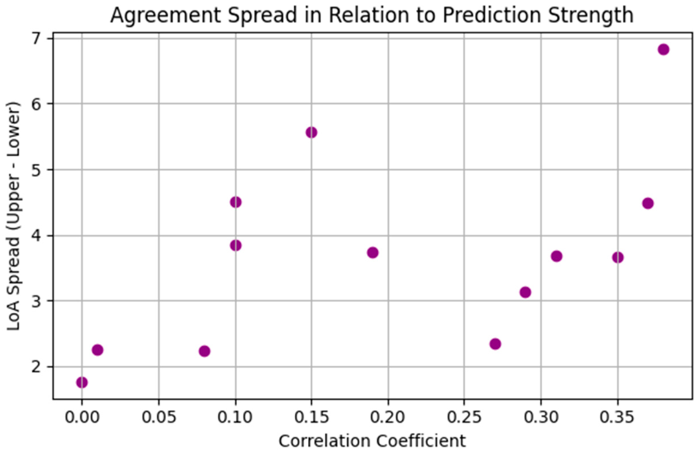
| Patient | Pearson Correlation | BA Mean | BA Lower LoA | BA Upper LoA |
|---|---|---|---|---|
| 1 | 0.38 | 0.01 | −3.41 | 3.42 |
| 2 | 0.29 | −0.02 | −1.58 | 1.55 |
| 3 | 0.00 | −0.07 | −0.95 | 0.81 |
| 4 | 0.15 | −0.07 | −2.85 | 2.71 |
| 5 | 0.35 | 0.02 | −1.82 | 1.85 |
| 6 | 0.27 | −0.02 | −1.19 | 1.16 |
| 7 | 0.19 | 0.02 | −1.85 | 1.89 |
| 8 | 0.10 | 0.00 | −1.92 | 1.92 |
| 9 | 0.37 | 0.02 | −2.22 | 2.26 |
| 10 | 0.01 | 0.00 | −1.13 | 1.13 |
| 11 | 0.08 | −0.01 | −1.13 | 1.11 |
| 12 | 0.31 | 0.00 | −1.84 | 1.85 |
| 13 | 0.10 | −0.29 | −2.54 | 1.97 |
Disclaimer/Publisher’s Note: The statements, opinions and data contained in all publications are solely those of the individual author(s) and contributor(s) and not of MDPI and/or the editor(s). MDPI and/or the editor(s) disclaim responsibility for any injury to people or property resulting from any ideas, methods, instructions or products referred to in the content. |
© 2025 by the authors. Licensee MDPI, Basel, Switzerland. This article is an open access article distributed under the terms and conditions of the Creative Commons Attribution (CC BY) license (https://creativecommons.org/licenses/by/4.0/).
Share and Cite
Vakitbilir, N.; Raj, R.; Griesdale, D.E.G.; Sekhon, M.; Bernard, F.; Gallagher, C.; Thelin, E.P.; Froese, L.; Stein, K.Y.; Kramer, A.H.; et al. Impact of Temporal Resolution on Autocorrelative Features of Cerebral Physiology from Invasive and Non-Invasive Sensors in Acute Traumatic Neural Injury: Insights from the CAHR-TBI Cohort. Sensors 2025, 25, 2762. https://doi.org/10.3390/s25092762
Vakitbilir N, Raj R, Griesdale DEG, Sekhon M, Bernard F, Gallagher C, Thelin EP, Froese L, Stein KY, Kramer AH, et al. Impact of Temporal Resolution on Autocorrelative Features of Cerebral Physiology from Invasive and Non-Invasive Sensors in Acute Traumatic Neural Injury: Insights from the CAHR-TBI Cohort. Sensors. 2025; 25(9):2762. https://doi.org/10.3390/s25092762
Chicago/Turabian StyleVakitbilir, Nuray, Rahul Raj, Donald E. G. Griesdale, Mypinder Sekhon, Francis Bernard, Clare Gallagher, Eric P. Thelin, Logan Froese, Kevin Y. Stein, Andreas H. Kramer, and et al. 2025. "Impact of Temporal Resolution on Autocorrelative Features of Cerebral Physiology from Invasive and Non-Invasive Sensors in Acute Traumatic Neural Injury: Insights from the CAHR-TBI Cohort" Sensors 25, no. 9: 2762. https://doi.org/10.3390/s25092762
APA StyleVakitbilir, N., Raj, R., Griesdale, D. E. G., Sekhon, M., Bernard, F., Gallagher, C., Thelin, E. P., Froese, L., Stein, K. Y., Kramer, A. H., Aries, M. J. H., & Zeiler, F. A. (2025). Impact of Temporal Resolution on Autocorrelative Features of Cerebral Physiology from Invasive and Non-Invasive Sensors in Acute Traumatic Neural Injury: Insights from the CAHR-TBI Cohort. Sensors, 25(9), 2762. https://doi.org/10.3390/s25092762